Using Space Geodesy to Constrain
Variations in Seismogenic Behavior on
Subduction Megathrusts
Thesis by Yunung Nina Lin
In Partial Fulfillment of the Requirements for the degree of
Doctor of Philosophy
CALIFORNIA INSTITUTE OF TECHNOLOGY Pasadena, California
2013
ii
iii
ACKNOWLEDGEMENTSI want to thank my two thesis advisors, Professor Mark Simons and Jean-Philippe Avouac, for the past six years of valuable advisement and support. Mark is so sharp in science and always sees through the core of any scientific topic. Jean-Philippe has a great mind and point of view about science that inspires me all the time. I learn from both of them in so many different aspects: the courses they offered during my first few years (Tectonic Geodesy from Mark and Geology of Earthquakes from Jean-Philippe), the moments that we sat down together and worked through the equations and codes, and the thoughts and ideas about science that they shared during official talks and casual conversations. Most important of all, as the saying “Example is better than percept” goes, they show me as the best examples what great scientists are, how they target scientific problems, and how they perceive the value of science. These are the fruits that I will walk away with and will accompany me through the rest of my career.
I also want to thank Professor Joann Stock, my academic advisor, for being my role model of a great scientist and a mother. The stories about how she took care of her babies and did great science at the same time always remind me that everything is possible, and that we ought not to set limits to ourselves. Her understanding of the difficulties that a female graduate student with babies may face, and the support and advices she offered, always give me courages to move on during my hard times.
My first year project advisor, Professor Kerry Sieh, now at Earth Observatory of Singapore, is another person that I owe gratitude to. He is a very close family friend (thanks for attending my wedding!) and a great scientist to work with. We had a lot of fun time together in Taiwan (2005), in Bandong, Indonesia (2006), in Singapore (2007) and in my first year at Caltech (2007-08).
iv
My labmates are the most important resources I go to whenever I encounter problems. Former members include Chris DeCaprio, Eric Hetland, Ravi Kanda, Sarah Minson, Anthony Sladen; current members include Piyush Agram, Zacharie Duputel, Junle Jiang, Romain Jolivet, Hilary Martens, Brent Minchew, Francisco Ortega, Bryan Riel and Jeff Thompson. Thank you so much for being supportive to me at all times.There are many other people who really make my life at Caltech, mostly former and current members of the Tectonics Observatory. They are Thomas Ader, Willy Amadom (and his wife Susan), Sylvain Barbot, Alan Chapman (and his wife Kelly), Nadaya Cubas, John Galetzka, Janet Harvey, Jamshid Hassanzadeh, Yihe Huang, Steve Kidder (and his wife Robin), Young-Hee Kim, Aron Meltzner, Lingsen Meng, Belle Philibosian (and her husband Adam), Steve Skinner, Marion Thomas, Zhongwen Zhan, and Dongzhou Zhang. Thank Tectonics Observatory for gathering so many interesting people to make the research life exciting and after-work life colorful.
And my most sincere thanks to the administrative and supportive staff: Mike Black, Dian Buchness, Leticia Calderon, Lisa Christiansen, Scott Dungan, Marcia Hudson, Rosemary Miller, Donna Mireles, and Heather Steele. Without their help, my life would be a lot more miserable with the crazy logistics and computer stuff.
Other important family friends who supported me during these six years include Wei-Ting Chen and Eh Tan (both former Caltech graduate students), Fan-Chi Lin (current GPS post-doc) and his families, and Yue-Gau Chen (my master thesis advisor at National Taiwan University). Their companion makes the transition from Taiwanese culture to American culturer much easier.
vi
ABSTRACTvii
bathymetric features on the downgoing plate are presently subducting, whereas theviii
TABLE OF CONTENTSAcknowledgements ... iii
Abstract ...vi
Table of Contents...viii
List of Illustrations ...xi
List of Tables... xiii
Introduction... 1
Seamounts ...3
Fracture Zones ...4
Fore-arc Depressions...5
From a Geodetic Perspective...6
References of Introduction... 8
Chapter I: A multiscale approach to estimating topographically correlated propagation delays in radar interferograms... 11
Abstract... 11
1.1 Introduction...12
1.2 A Multiscale Approach to Estimating Topographically Correlated Delays ... 15
1.2.1 Model ... 15
1.2.2 Estimation Approach... 17
1.2.3 Synthetic Test ...19
1.3 Correcting Real Interferograms... 22
1.3.1 Long Valley Caldera ... 23
1.3.2 The 2007 Tocopilla Earthquake, Chile... 26
1.4 Discussion and Conclusion ... 28
References of Chapter I ... 30
Chapter II: PCAIM joint inversion of InSAR and groundbased geodetic time series: Application to monitoring magmatic inflation beneath the Long Valley Caldera... 46
Abstract... 46
2.1 Introduction...47
2.2 Joint Inversion Using PCAIM ... 49
2.2.1 PCAIM Principles... 49
2.2.2 PCAIM Decomposition... 50
2.2.3 Results of the Joint Inversion ...52
2.3 Discussion and Conclusion ...53
References of Chapter II...56
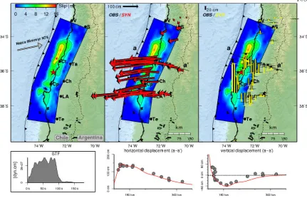
Chapter III: Coseismic and Postseismic Slip Associated with the 2010 Maule Earthquake, Chile: Characterizing the Arauco Peninsula Barrier Effect... 62
Abstract... 62
ix
3.2 The 2010 Maule Earthquake and Its Seismotectonic Settings ... 66
3.3 Data ... 69
3.4 Coseismic Slip Model ... 70
3.5 Postseismic Slip Model...73
3.6 Discussion ... ...76
3.6.1 Postseismic Moment Release...76
3.6.2 Spatial Friction Variations and the Earthquake Barrier ...78
3.6.3 Arauco Peninsula Uplift...81
3.6.4 Limitations ... 83
3.7 Conclusion... 86
References of Chapter III ... 88
Chapter IV: Interseismic plate coupling in the eastern Makran Subduction Zone... 113
Abstract... 113
4.1 Introduction... 114
4.2 Tectonic Settings of the Eastern Makran Subduction Zone... ... 116
4.3 Data Processing ... 119
4.3.1 Atmospheric Phase Screen (APS) Correction ...120
4.3.2 Ocean Tidal Loads (OTL) Correction ...123
4.4 Time Series Analysis...125
4.5 Interseismic Coupling Models ...126
4.6 Discussion ... ...130
4.7 Conclusion...132
References of Chapter IV...134
Concluding Thoughts... 157
Appendix A: Supplementary Material of Chapter II...158
A.1 Comparison of Simultaneous and Iterative Decompositions...158
A.2 Comparison of InSAR-only, EDM-only and InSAR + EDM Joint Inversions ... ...159
Appendix B: Supplmentary Material of Chapter III...164
B.1 Data Selection and Processing...164
B.1.1 GPS Observations ...164
B.1.2 InSAR...167
B.2 Inversion Models ... 172
B.2.1 Coseismic Model ... 172
B.2.2 Postseismic Model ... 173
B.3 Effects of Approximate Green’s Function...183
B.4 Resolution of Updip Slip Extent from Tsunami Data ...184
B.5 Slip Potency Test for Shallow Slip ...185
B.6 Comparison between Slip Models and Aftershock Focal Mechanisms ...188
References of Appendix B ...189
Appendix C: Supplementary Material of Chapter IV...192
xi
LIST OF ILLUSTRATIONSNumber Page
1. 1 Original and decomposed topography and interferogram ... 34
1.2 B vs T plot ...35
1.3 Reference map of Long Valley Caldera ... 36
1.4 A schematic description of the construction of the synthetic interferometry ...37
1.5 Comparison of K values in a synthetic test ... 38
1.6 Comparison of decomposed turbulent signals with different scale distance Lc... 39
1.7 KT time series derived from multiscale approach ... 40
1.8 Comparison between observed and predicted Kigram...41
1.9 Comparison between the original and corrected interferograms in Long Valley Caldera example... 42
1.10 Scatter plots (phase vs. topography) between two real cases, Long Valley Caldera and Tocopilla, and two synthetic examples ... 43
1.11 Reference map of the 2007 Tocopilla earthquake ... 44
1.12 Comparison between the original and corrected interferograms in the Tocopilla example...45
2. 1 Basemap of Long Valley Caldera and the PCA decomposition ...59
2.2
r2vs the number of PCA components used ... 602.3 Reconstructed time series and residuals ...61
3. 1 Basemap of the study area in south-central Chile...97
3.2 Secular velocities, coseismic and postseismic deformation from GPS observations ... 99
3.3 ALOS PALSAR acquisitions used in this study ... 100
3.4 Original, resampled and modeled InSAR data... 101
3.5 Seismic waveforms and the coseismic slip model...102
3.6 Coseismic slip model and fits to GPS observations...103
3.7 Tsunameter records as predicted by coseismic slip model ...104
3.8 Postseismic times series of selected GPS stations...105
3.9 Comparison of postseismic slip models with different datasets ...106
3.10 Postseismic-to-coseismic energy release ratio vs coseismic moment and sediment thickness ... 108
3.11 Normalized time-dependent fault slip ... 110
3.12 Topography, deformation and uplift/subsidence rate of the Arauco Peninsula ...111
4. 1 Basemap of the Makran subduction zone...143
xii
4.3 Baseline plots for ENVISAT tracks used in this study ...146
4.4 An example of the comparison plot between the ECMWF delays, MERIS wet delays calibrated with ECMWF data, ocean tidal loads corrections, and the interferograms ... 147
4.5 Post-correction images...148
4.6 One example of the LOS displacement from ocean tidal loads...149
4.7 The LOS velocities and uncertainties obtained from the large ensemble of interferograms ...150
4.8 The LOS velocities and uncertainties obtained from the small ensemble of interferograms ... 151
4.9 An example plot of RMS residuals versus model roughness...152
4.10-1 The projected profile and interseismic coupling models from N10E convergent azimuth...153
4.10-2 The projected profile and interseismic coupling models from due north convergent azimuth...154
4.10-3 The projected profile and interseismic coupling models from N8W convergent azimuth ... 155
4.11 Cumulative moment deficit since last event as a function of distance along trench...156
A. 1 Comparison of simultaneous and iterative decompositions ...162
A.2 Comparison of the first 3 components from the joint, InSAR-only and EDM-only principal component decomposition ...163
B.1-1 The vertical component of cGPS time series, northern section ...169
B.1-2 The vertical component of cGPS time series, central section...170
B.1-3 The vertical component of cGPS time series, southern section ...171
B.2 Comparison of fault geometry from different models ... 177
B.3 Results from geodetic-only inversion ...178
B.4 Checkerboard test for the geodetic-only coseismic inversion ...179
B.5 Comparison between postseismic fault geometry and aftershocks 180 B.6 Postseismic model sensitivity ... 181
B.7 Checkerboard test for postseismic inversion...182
B.8 Inversion test for wrong rheology approximations...183
B.9 Tsunami wavefronts propagated from the deep-ocean buoys ...184
B.10 L-curve for slip potency test...185
B.11 Slip models for different slip potency constraints...187
B.12 Comparison between postseismic slip models and focal mechanisms for Maule aftershocks ...188
C.1 T220 large ensemble interferogram...192
C.2 T449 large ensemble interferogram...194
C.3 T177 large ensemble interferogram...196
C.4 T406 large ensemble interferogram...198
C.5 T220 small ensemble interferogram...200
C.6 T449 small ensemble interferogram...201
C.7 T177 small ensemble interferogram... 202
xiii
LIST OF TABLESNumber Page
1
I n t r o d u c t i o n
Determining the spatial extent and temporal evolution of seismic ruptures, as well as the physical parameters controlling their extent and locations, has been a theme in earthquake physics over the past three decades. It is generally observed that large earthquakes consist of subevents, relatively compact patches with locally high slip, called ‘asperities.’ The term “seismic asperity” was first defined by Kanamori [1978] to describe “geometrical asperities, heterogeneities of the frictional strength or a combination (of both)” on the fault plane. A complementary concept is that of a “barrier,” defined as the region that does not fail during the mainshock [Das and Aki, 1977; Kanamori, 1986]. The asperity and barrier models were originally two separate concepts used in the context of dynamic failure properties [Lay et al., 1982]. However, these concepts are now frequently combined to describe spatial, mainly along-strike variations of seismic and aseismic regions on the subduction interface. The spatial distribution of asperities and barriers may potentially bound the rupture area and moment release for future large earthquakes; their temporal evolution may help define any relationship between a single seismic cycle and long-term geologic features. The underlying controls for this heterogeneity in style of fault slip are directly related to the fundamental physical properties of the subduction zone. Imaging the spatial distribution of seismic asperities and zones of aseismic creep is therefore essential to advance our understanding of the seismic behavior of faults and governing physics.
2
the subduction interface. More explicitly, it states that shear tractions on the fault are mainly dependent on the effective normal stresses. Scholz and Campos [1995] use this model to predict the seismogenic behaviors across different subduction zones, although notable exceptions exist [Scholz and Campos, 2012].Another model proposes a different hypothesis regarding the relationship between the state of stress on the megathrust and seismogenic behavior. This model suggests that “spatial variations in frictional properties on the plate interface control trench-parallel variations in fore-arc topography, gravity, and seismogenic behavior” [Song and Simons, 2003] and that “forearc basins may be useful indicators of long-term seismic moment release” [Wells et al., 2003] (although in Wells et al. [2003] they attribute this relationship to subduction erosion). Song and Simons [2003] observed strong correlation of negative gravity and topography anomalies with seismogenic patches in large earthquakes, and related the distribution of seismic asperities within individual subduction zones to regions of increased shear traction. They argued that since negative gravity and topography anomalies are associated with decreased normal stress, the regions of shear traction increase are more likely due to increases in the effective coefficient of friction, although normal tractions may also modulate the shear tractions. This model is consistent with the inferred slip distribution of most large earthquakes; but again, exceptions also exist (e.g., the 2005 Mw 8.7 Nias in Sumatra and the 2011 Mw 9.0 Tohoku-oki in Japan).
3
Thus, Scholz and Campos [1995] and Song and Simons [2003] may represent end-member models. Before delving into these models in detail, it is important to recognize ongoing controversies associated with the role of commonly found bathymetric features: subducting seamounts, subducting fracture zones, and fore-arc depressions.Seamounts
Many studies infer a strong correlation between subducted seamounts and either seismic asperities (e.g., Ichinose et al., [2007] for the 1964 Alaska earthquake) or barriers (e.g..
4
Various attempts have been made to explain how seamount subduction influences plate coupling. Analogue models suggest that the dense fracture network generated by seamount subduction would favor fluid expulsion and induce a decrease in the fluid pressure and effective basal friction, possibly leading to lower coupling [Dominguez et al., 2000]. This conclusion is further supported by the complexity of moment rate functions for events in areas of subducting seamounts in Costa Rica [Wang and Bilek, 2011].Yang et al. [2012] numerically modeled a seamount as a strong patch of high effective normal stress within a rate-and-state friction subduction zone setting. Their result suggests that a seamount may act as a rupture barrier whose efficiency depends on both the increase of effective normal stress and the seamount-to-trench distance. Whenever the stress state becomes favorable, ruptures can also nucleate on the same seamount. This numerical model may explain many of the past controversies, although the model does not associate seamounts with any specific rate-and-state frictional properties, and therefore how these properties may influence the asperity and barrier effect of a seamount remains unknown.
Fracture Zones
5
highs (mostly fracture zones with some ridges) on the downgoing plate and rupture extents of large earthquakes [Carena 2011; Contreras-Reyes and Carrizo, 2011], while the exact mechanism is still debated. Some consider that incoming fracture zones may enhance the flux of water into the subduction zone and may induce pore pressure changes or hydration and hence serpentinization of ultramafic rocks on the subducting plate [Chlieh et al., 2008; Contreras-Reyes et al., 2008], both leading to variations in the frictional behavior on the plate interface [Escartin et al., 1997], while others propose that the bathymetric steps across the fracture zone constitute a major geometric control over the rupture extent, similar to the lateral ramps associated with crustal faults [Carena 2011].Fore-arc Depressions
6
From a Geodetic Perspective
The ambiguous evidence associated with the Scholz and Campos [1995] and Song and Simons [2003] models indicates that the underlying physical process is more complicated than a simple dichotomy between the normal-stress dominant and frictional-property dominant interplate coupling. It is likely that the two models are end members over a wide spectrum, in which two or more major factors contribute to controlling the seismogenic process. Our ability to disentangle the multiple potential controls on seismogenic behavior of the megathrust relies intimately on our ability to reliably resolve the distribution of coseismic and aseismic fault slip on subduction megathrusts. As elucidated by several studies [e.g. Wells et al., 2003; Singh et al., 2011], some of the aforementioned disputes may result from the insufficient resolution of coseismic slip or interseismic coupling models and/or plate interface topography due to poor data quality, especially for earlier historic events.
7
resolution can provide detailed mapping of the source parameters and the associated temporal evolution. The inversion is carried out via a Principal Component Analysis based Inversion Method (PCAIM) [Kositsky and Avouac, 2010].8
References of IntroductionBaba, T., Y. Tanioka, P. R. Cummins, and K. Uhira (2002), The slip distribution of the 1946 Nankai earthquake estimated from tsunami inversion using a new plate model, Phys. Earth Planet. Inter., 132(1-3), 59-73.
Béjar-Pizarro, M., A. Socquet, R. Armijo, D. Carrizo, J. Genrich, and M. Simons (2013), Andean structural control on interseismic coupling in the North Chile subduction zone,
Nat. Geosci., doi: 10.1038/ngeo1802.
Carena, S. (2011), Subducting-plate Topography and Nucleation of Great and Giant Earthquakes along the South American Trench, Seismol. Res. Lett., 82(5), 629-637, doi: 10.1785/gssrl.82.5.629.
Chlieh, M., J. P. Avouac, K. Sieh, D. H. Natawidjaja, and J. Galetzka (2008), Heterogeneous coupling of the Sumatran megathrust constrained by geodetic and paleogeodetic measurements, J. Geophys. Res., 113(B5), B05305, doi: 10.1029/2007jb004981.
Chlieh, M., H. Perfettini, H. Tavera, J.-P. Avouac, D. Remy, J.-M. Nocquet, F. Rolandone, F. Bondoux, G. Gabalda, and S. Bonvalot (2011), Interseismic coupling and seismic potential along the Central Andes subduction zone, J. Geophys. Res., 116(B12), B12405, doi: 10.1029/2010JB008166.
Contreras-Reyes, E., and D. Carrizo (2011), Control of high oceanic features and subduction channel on earthquake ruptures along the Chile-Peru subduction zone, Phys. Earth Planet. Inter., 186(1-2), 49-58.
Contreras-Reyes, E., I. Grevemeyer, E. R. Flueh, and C. Reichert (2008), Upper lithospheric structure of the subduction zone offshore of southern Arauco peninsula, Chile, at ~38°S, J. Geophys. Res., 113(B7), B07303, doi: 10.1029/2007JB005569.
Das, S., and K. Aki (1977), Fault plane with barriers - versatile earthquake model, J. Geophys. Res., 82(36), 5658-5670, doi: 10.1029/JB082i036p05658.
Dominguez, S., J. Malavieille, and S. E. Lallemand (2000), Deformation of accretionary wedges in response to seamount subduction: Insights from sandbox experiments,
Tectonics, 19(1), 182-196, doi: 10.1029/1999tc900055.
Escartin, J., G. Hirth, and B. Evans (1997), Nondilatant brittle deformation of serpentinites: Implications for Mohr-Coulomb theory and the strength of faults, J. Geophys. Res., 102(B2), 2897-2913, doi: 10.1029/96jb02792.
9
Ichinose, G., P. Somerville, H. K. Thio, R. Graves, and D. O'Connell (2007), Rupture process of the 1964 Prince William Sound, Alaska, earthquake from the combined inversion of seismic, tsunami, and geodetic data, J. Geophys. Res., 112(B7), doi: 10.1029/2006jb004728.Kanamori, H. (1978), Use of seismic radiation to infer source parameters, USGS Open File Report 78-380, 283-318 pp.
Kodaira, S., N. Takahashi, A. Nakanishi, S. Miura, and Y. Kaneda (2000), Subducted seamount imaged in the rupture zone of the 1946 Nankaido earthquake, Science,
289(5476), 104-106, doi: 10.1126/science.289.5476.104.
Kodaira, S., A. Nakanishi, J. O. Park, A. Ito, T. Tsuru, and Y. Kaneda (2003), Cyclic ridge subduction at an inter-plate locked zone off central Japan, Geophys. Res. Lett., 30(6), doi: 10.1029/2002gl016595.
Kodaira, S., T. Iidaka, A. Kato, J. O. Park, T. Iwasaki, and Y. Kaneda (2004), High pore fluid pressure may cause silent slip in the Nankai Trough, Science, 304(5675), 1295-1298, doi: 10.1126/science.1096535.
Kodaira, S., et al. (2002), Structural factors controlling the rupture process of a megathrust earthquake at the Nankai trough seismogenic zone, Geophys. J. Int., 149(3), 815-835.
Kositsky, A., and J. P. Avouac (2010), Inverting geodetic time-series with a principal component analysis-based inverison method (PCAIM), J. Geophys. Res., 115, B03401, doi: 10.1029/2009JB006535.
Lange, D., F. Tilmann, A. Rietbrock, R. Collings, D. H. Natawidjaja, B. W. Suwargadi, P. Barton, T. Henstock, and T. Ryberg (2010), The fine structure of the subducted Investigator Fracture Zone in western Sumatra as seen by local seismicity, Earth Planet. Sci. Lett., 298(1-2), 47-56, doi: 10.1016/j.epsl.2010.07.020.
Lay, T., H. Kanamori, and L. Ruff (1982), The asperity model and the nature of large subduction zone earthquakes, Earthquake Pred. Res., 1(1), 3-71.
Loveless, J. P., M. E. Pritchard, and N. Kukowski (2010), Testing mechanisms of subduction zone segmentation and seismogenesis with slip distributions from recent Andean earthquakes, Tectonophysics, 495(1–2), 15-33, doi: 10.1016/j.tecto.2009.05.008. Mochizuki, K., T. Yamada, M. Shinohara, Y. Yamanaka, and T. Kanazawa (2008), Weak interplate coupling by seamounts and repeating M~7 earthquakes, Science, 321(5893), 1194-1197, doi: 10.1126/science.1160250.
Moreno, M., et al. (2011), Heterogeneous plate locking in the South-central Chile subduction zone: Building up the next great earthquake, Earth Planet. Sci. Lett., 305(3-4), 413-424.
Perfettini, H., et al. (2010), Seismic and aseismic slip on the Central Peru megathrust,
10
Rosenau, M., and O. Oncken (2009), Fore-arc deformation controls frequency-size distribution of megathrust earthquakes in subduction zones, J. Geophys. Res., 114, doi: 10.1029/2009jb006359.Ruff, L. J., and B. W. Tichelaar (1996), What controls the seismogenic plate interface in subduction zones?, in Subduction Top to Bottom, edited, pp. 105-111, AGU, Washington, DC.
Scholz, C. H., and J. Campos (1995), On the mechanism of seismic decoupling and back-arc spreading at subduction zones, J. Geophys. Res., 100(B11), 22103-22115, doi: 10.1029/95jb01869.
Scholz, C. H., and C. Small (1997), The effect of seamount subduction on seismic coupling,
Geology, 25(6), 487-490, doi: 10.1130/0091-7613(1997)025<0487:TEOSSO>2.3.CO;2. Scholz, C. H., and J. Campos (2012), The seismic coupling of subduction zones revisited, J. Geophys. Res., 117, doi: 10.1029/2011jb009003.
Singh, S. C., et al. (2011), Aseismic zone and earthquake segmentation associated with a deep subducted seamount in Sumatra, Nat. Geosci., 4(5), 308-311, doi: 10.1038/ngeo1119. Sladen, A., H. Tavera, M. Simons, J. P. Avouac, A. O. Konca, H. Perfettini, L. Audin, E. J. Fielding, F. Ortega, and R. Cavagnoud (2010), Source model of the 2007 M-w 8.0 Pisco, Peru earthquake: Implications for seismogenic behavior of subduction megathrusts, J. Geophys. Res., 115, B02405, doi: 10.1029/2009JB006429.
Song, T. R. A., and M. Simons (2003), Large trench-parallel gravity variations predict seismogenic behavior in subduction zones, Science, 301(5633), 630-633, doi: 10.1126/science.1085557.
Wang, K., and Y. Hu (2006), Accretionary prisms in subduction earthquake cycles: The theory of dynamic Coulomb wedge, J. Geophys. Res., 111(B6), B06410, doi: 10.1029/2005jb004094.
Wang, K. L., and S. L. Bilek (2011), Do subducting seamounts generate or stop large earthquakes?, Geology, 39(9), 819-822, doi: 10.1130/g31856.1.
Wells, R. E., R. J. Blakely, Y. Sugiyama, D. W. Scholl, and P. A. Dinterman (2003), Basin-centered asperities in great subduction zone earthquakes: A link between slip, subsidence, and subduction erosion?, J. Geophys. Res., 108(B10), 2507, doi: 10.1029/2002JB002072. Yang, H. F., Y. J. Liu, and J. Lin (2012), Effects of subducted seamounts on megathrust earthquake nucleation and rupture propagation, Geophys. Res. Lett., 39, doi: 10.1029/2012gl053892.
11
C h a p t e r 1
A MULTISCALE APPROACH TO ESTIMATING TOPOGRAPHICALLY CORRELATED PROPAGATION DELAYS IN RADAR INTERFEROGRAMS
Originally published in Lin, Y.-N. N., M. Simons, E. A. Hetland, P. Muse, and C. DiCaprio (2010), A multiscale approach to estimating topographically correlated propagation delays in radar interferograms, Geochem. Geophys. Geosyst., 11(9), Q09002, doi: 10.1029/2010GC003228.
Abstract
12
determine the bands wherein correlation between topography and phase is significant and stable. When possible, our approach also takes advantage of any inherent redundancy provided by multiple interferograms constructed with common scenes. We define a unique set of component time intervals for a given suite of interferometric pairs. We estimate an internally consistent transfer function for each component time interval, which can then be recombined to correct any arbitrary interferometric pair. We demonstrate our approach on a synthetic example and on data from two locations: Long Valley Caldera, California, which experienced prolonged periods of surface deformation from pressurization of a deep magma chamber, and one coseismic interferogram from the 2007 Mw 7.8 Tocopilla earthquake in northern Chile. In both examples, the corrected interferograms show improvements in regions of high relief, independent of whether or not we precorrect the data for a source model. We believe that most of the remaining signals are predominately due to heterogeneous water vapor distribution that requires more sophisticated correction methods than those described here.1.1 Introduction
Interferometric Synthetic Aperture Radar (InSAR) images are widely used in the analysis of tectonic deformation, magmatic activity, flow of glaciers, and other surface deformation processes (for reviews, see Massonnet et al. [1994], Burgmann et al. [2000], Hanssen
13
of water vapor, also known as “wet delays,” contribute the most to the neutral atmospheric propagational delays [Bevis et al., 1992]. Recent study also shows that hydrostatic delays, which depends on the pressure to temperature ratio, vary significantly at low elevation and cannot be neglected [Doin et al., 2009]. Ionospheric effects result from spatio-temporal variations in ionospheric electron density. These effects are in general more obvious in the higher latitude and in the Lband SAR data than the Cband SAR, due to the dispersive nature of the atmospheric medium [Gray et al., 2000]. Wet delays and hydrostatic delays may strongly obscure tectonic signals when the signal amplitude is small as is frequently the case with interseismic deformation. For example, in twopass interferometry, a 20% change in humidity may result in 10 cm of deformation error [Zebker et al., 1997], thereby compromising the effectiveness for InSAR to detect mmtocm scale deformation. Wet delays and hydrostatic delays are nondispersive and therefore the multi-wavelength approach generally used to correct for GPS ionospheric biases cannot be applied to tackle this problem [Zebker et al., 1997].
One way to mitigate the tropospheric delay problem is to average N independent interferograms, since the neutral atmospheric signals are uncorrelated over timescales longer than 1day [Zebker et al., 1997; Emardson et al., 2003]. This simple technique can
14
this approach is subjective, leading to the concern of smoothing out signals over the same time scales as the noise.Other studies propose more complicated but direct methods for estimating and removing the effects of wet delays. Proposed methods include use of GPS data [Onn and Zebker,
2006] and radiometric data to produce zenith path delay difference maps for InSAR atmospheric correction, for instance using either MODIS (MODerate-resolution Imaging Spectroradiometer) [Li et al., 2005, 2006a], or MERIS (MEdium Resolution Image Spectrometer, for ENVISAT system only) [Li et al., 2006b, 2006c]. Other approaches use weather models together with radiometric data to generate an instant water vapor map, such as MERIS with MM5 (Mesoscale Meteorological Model) [Puysségur et al., 2007], or use a weather model only to predict atmospheric delays [Foster et al., 2006]. These imagerybased or modelbased approaches may provide estimates of water vapor distribution from independent data sources or models at the time the SAR image was acquired. However, imagerybased approaches have limited application for older SAR images. MODIS and MERIS were launched in 1999 and 2002, respectively. Radiometric systems require solar illumination, so they can not be used to correct for SAR images acquired at night. Some calibration statement is also necessary for the user to accommodate the radiometric data to different study areas. GPSbased approaches are limited by the density and existence of GPS stations in some remote areas. Moreover, the efficacy of modeling-based approaches are still debated, especially the extent to which they consistently reduce or add noise to interferometric observations.
15
approach focuses on mitigating the effects of the timevariable vertically stratified component of the atmospheric delays, as described by Hanssen [2001]. Correction of the static component is relatively straightforward and efficient, and in some cases can be very effective. In a study of the Lake Mead area, Nevada, Cavalié et al. [2007] showed that static tropospheric delays can be estimated by analyzing the correlation between phase and topography. (To be more accurate, it is a correlation between phase change and topography, but for simplicity we use “phase” to refer to “phase change”). This method, however, does not always work well because in some cases phase does not seem linearly related to topography due to multiple tectonic/nontectonic sources and confounding effects of delays due to turbulent atmospheric circulation.Our study proposes an improved method that is less sensitive to all these confounding factors. We use a multiscale approach to estimate variations in topographicallycorrelated propagation delays. This approach is based on the same assumption made by earlier works of a linear relationship between phase and topography. We first test our approach in a synthetic example, and validate that in regions where there is no strong turbulent mixing, this approach can serve as the first order correction. We then demonstrate our method with examples from the Long Valley Caldera in California, and northern Chile.
1.2 A Multiscale Approach to Estimating Topographically Correlated Delays
1.2.1 Model
16
temperature (T), humidity and water vapor content in the lowermost atmosphere between two SAR acquisitions [Hanssen, 2001]. For a vertically stratified troposphere model, if elevation changes across the scene, propagation delays vary at different elevation with a rate increasing with water vapor content and P/T ratio [Doin et al., 2009]. In contrast to the effect of turbulent mixing, this vertical stratification is considered static over a given area throughout a certain period of time. As the concentration of water vapor generally decreases exponentially with elevation, the theoretical delay curve is an exponential function of elevation [Delacourt et al., 1998]. In an interferogram subject to only static tropospheric delays, the signal is the difference between the delay curves for two individual SAR acquisitions. If we take a Taylor series expansion over the resultant exponential function, and ignore the second order and higher terms, we can derive a simple linear relationKh
b
(1-1)17
1.2.2 Estimation ApproachOur approach explicitly recognizes that various length scales, , should have different sensitivities to different sources of confounding noises. For example, very large (>100 km) may be more sensitive to other processes such as tidal loading [DiCaprio and Simons, 2008] or orbital error, whereas the smallest (≤2 km) may not be very sensitive to larger
scale tropospheric signals. Surface deformation resulting from tectonic, magmatic or glacial processes also has a rich scaledependent spectrum. In the presence of all these confounding factors, given that K is assumed to be a global property, there should be a reasonable range of in which the value of K almost stays constant and is independent of . Therefore, we can take advantage of the multiscale perspective to robustly estimate a spatially constant K which is relatively insensitive to confounding processes.
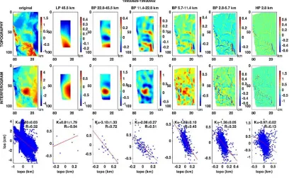
To begin with, we decompose both topography and interferogram into different length scales (Figure 1.1). We generate bandpassed images by applying a series of Gaussian filters with different spatial scales and taking the difference between two neighboring scales. We choose filter limits that scale with integer powers of two (in units of integer numbers of pixels). To properly represent the amount of information carried in each channel, we resample them according to the ShannonNyquist sampling theorem. We use the resampled point sets from selected bandpass channels to estimate K.
18
)
(
)
(
ib
igramK
igramh
i
(1-2)where h(i) and
(
i)
are the ith bandpassed components of h and
. bigram andKigram denote the bias term and transfer function of each interferogram. When multiple
interferograms are available for the same region we must estimate a consistent set of values for K. We do so by defining a unique set of component time intervals,
T
, for a suite of interferograms (Figure 1.2). Each
T
has a corresponding bT and KT, which represents the internally consistent b and K changes over this time interval. Next we construct the linear system
)
(
)
(
)
(
)
(
1
1
0
0
0
0
1
1
0
0
1
1
0
0
1
1
)
(
)
(
0
0
0
0
)
(
)
(
0
0
)
(
)
(
0
0
)
(
)
(
1 2 1 1 1 2 1 2 2 2 1 2 2 1 1 3 2 1 3 2 1 n m n T T T T T T T T n m n m n n p pb
b
b
b
K
K
K
K
h
h
h
h
h
h
h
h
(1-3)
where hm(n) represents the n selected decomposed bands of topography corresponding to
m interferograms, and
m(
n)
represents the n selected decomposed bands of minterferograms, while KTp and bTp represent the transfer function and bias term for the
19
We assume that there exist minor outliers in the data due to unwrapping errors or other measurement or processing defects. Under this assumption, an outlierresistant L1norm regression is a better choice than leastsquares regression. In practice, we use a convex optimization algorithm (available online as Matlab package cvx) (M. Grant and S. Boyd, CVX: Matlab software for disciplined convex programming, 2009, available at http://stanford.edu/boyd/cvx) for L1 regression to derive the best solution of KT [Boydand Vandenberghe, 2004]. Since there is no analytical equation to define model errors of L1norm regression, we estimate the standard error of KT (
T
K
) using a bootstrappingtechnique. Given that InSAR data are correlated in space, ideally we should include the full covariance matrix into our regressions. However, because we apply a multiscale decomposition by using a series of Gaussian filters, there is an issue of transforming the covariance matrix into each bandpass channel. The details are beyond the scope of this study, so we ignore data covariance in our regressions. The reader should keep in mind that the standard errors of K may be larger than what we present if the full covariance is considered. Finally, we form the time series of KT by choosing an arbitrary origin (we use
zero here) for the whole series and sequentially adding up all KT. Once the time series of
the transfer function KT is formed, it is easy to determine the
K
igram of an interferogramfrom any arbitrary pair of SAR scenes.
1.2.3 Synthetic Test
20
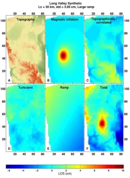
synthetic interferogram include tectonic (magmatic inflation), static topographicallycorrelated delays, turbulent mixing and ramp signals. We construct the tectonic signals by using a point source of inflation in an elastic halfspace [Mogi, 1958]. We assume a source depth at 10.5 km, consistent with Fialko et al. [2001]. As for turbulent mixing signals, several predetermined noise covariance functions have been proposed, such as a power law or an exponential decay [Hanssen, 2001; Emardson et al., 2003; Lohman and Simons, 2005]. Here we chose the expression of Lohman and Simons [2005]
c ij L
L ij d
e
C
/ (1-4)n c
vu
n
n
1/2 (1-5)where ij d
C
andL
ij are the covariance and distance between the ith and jth points, Lc is thescale distance, nn is uncorrelated noise, and v and u are the matrices of eigenvectors and
eigenvalues of Cd, respectively. We assume a ramp that varies bilinearly in space. The
constructed ramp has a major gradient in the NWSE direction, mimicking possible effects due to orbital error or horizontal water vapor gradients from north to south.
There are three major parameters that we vary to see how they influence the estimate of K. The first one is the standard deviation of non-correlated noise nn. The value is set to be
between 0 and 5 cm. The second parameter is the amplitude of the ramp. A small ramp has values between −0.5 to 0.5 cm, close to the amplitude of tectonic signals. A large ramp has amplitude 10 times the small ramp. The last parameter is the characteristic length scale, Lc,
21
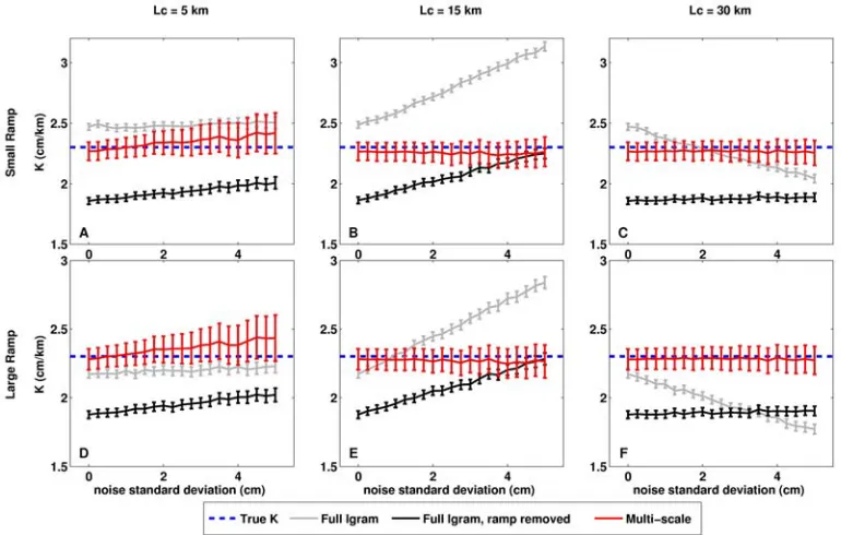
Estimates from real observations suggest a scale distance usually between 5 and 30 km [Lohman and Simons, 2005]. We test values of 5 km, 15 km and 30 km.Figure 1.4 shows one realization of our synthetic interferograms. We project all the components into the lineofsight direction and combine them together. In total we generate 120 interferograms and retrieve K values from each of them by using our multiscale approach. We then compare our results with the K values derived from a full (not multiscale) interferogramtopography correlation, with either ramp retained or ramp removed (Figure 1.5). The results show that the multiscale approach gives a stable estimate of K values regardless of noise strength. For the cases where Lc = 5 km, K values slightly
deviate to higher values from the true K as the noise increases, but are still within the error bars. In general, at greater noise levels, the multiscale approach tends to estimate transfer functions that are smaller than the real values. This tendency to underestimate K
means that the multiscale approach is a more conservative method, so that in most cases it will undercorrect rather than overcorrect the topographicallycorrelated tropospheric signals.
22
Lc also has some influence on the multiscale method. The K values retrieved using the
multiscale approach seem to be more stable at larger Lc. To explain this phenomenon, we
compare the decomposed turbulent signals of different Lc (Figure 1.6). At Lc = 5 km,
turbulent signals have more evenly spread amplitudes in all decomposed bands. As Lc
increases, turbulent signals become more concentrated in the longwavelength channels. Therefore in general, at large Lc, estimation of K should be less influenced by turbulent
mixing effects, but still depends on how the turbulent peaks and troughs randomly correlate to topography. In real cases, unfortunately, most turbulent signals are frequently related to topography. The user should hence keep in mind that the retrieved K is likely to be degraded from the “true” K, with the level of deviation depending on the characteristic length scale and amplitude (standard deviation) of turbulent signals.
To summarize the results from the synthetic test, we find that a multiscale approach provides a more robust way to estimate the transfer function, K. This approach is insensitive to phase ramps, and therefore can yield better estimates of K when orbital error or longwavelength deformation signals are present. Of course, as just alluded to, there may be a slight deviation of K depending on the characteristic length scale and amplitude of turbulent signals.
1.3 Correcting Real Interferograms
23
signals. We test the robustness of K by removing the magmatic inflation signals from the interferograms. We also use this example to emphasize the stability of our algorithm in the presence of largeamplitude turbulent noise. Our second example, the 2007 Tocopilla earthquake (northern Chile), has “rich” tectonic signals that cover a large area and wide range of wavelengths. We show how the K values may vary with scene sizes and comment on whether it is reasonable to correct a largesize interferogram with a unique value of K. Since this study focuses on estimating topographicallycorrelated tropospheric signals, we do not discuss in detail the geophysical aspects of the two study cases.1.3.1 Long Valley Caldera
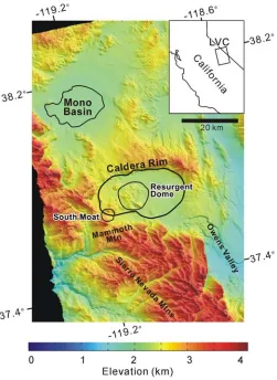
Long Valley Caldera has experienced two phases of volcanic unrest since 1989. The first phase started rapidly in 1989, and slowly decayed through the early 1990s. The second phase started slowly in mid1997, climaxed in late 1997, and returned to quiescence by mid
1998. During the second phase, it first showed an exponential growth increase in mid
April, and an exponential growth decay in late November 1997, cumulating in ∼10 cm of uplift [Newman et al., 2001; Hill et al., 2003; Langbein, 2003].
24
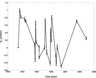
this case, our correction approach may serve as the best available tool to mitigate these static delays for older interferograms.We analyzed 65 interferograms based on 24 ERS acquisitions between 1992 and 2006. We tried to minimize the number of interferograms according to several criteria: (1) the length of the perpendicular component of baseline (B) should be less than 300 m; (2) the date of acquisition should lie outside the winter season, according to snow precipitation records (Daily snow depth data of Rock Creek Lakes (RCK), California Data Exchange Center, Department of Water Resources, available at http://cdec.water.ca.gov/cgiprogs/ staMeta?station_id=RCK); and (3) the difference in Doppler frequency between two acquisitions must be less than 900 Hz. The third criterion is particularly important, because the Doppler frequency starts to wander over a large range of values starting in 2001 [Meadows et al., 2007].
We first carried out a multiscale decomposition of topography and interferograms with 720 m mean ground resolution. The length scales thus chosen, from low to high frequencies, are >44.5, 22.2–44.5, 11.1–22.2, 5.6–11.1, 2.8–5.6 and <2.8 km. As we assume that smaller length scales (l ≤ 2 km) may not be sensitive enough to largerscale tropospheric signals, there is no need to use higher data ground resolution, which also saves computation time. Of course, once K is estimated, we can apply the correction to the full resolution interferogram. We then constructed and solved the linear system of equations (1-3). The time it takes to solve this linear system (65 interferograms) on an average PC is currently usually less than half an hour. We apply a bootstrapping technique [Tichelaar and Ruff, 1989] and derive the standard errors for KT, with the average as
25
T
K are nearly identical to those estimated on an interferogram by interferogram basis,
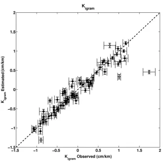
except for few outliers (Figure 1.8). After examining outlier interferograms individually, we found that these interferograms have larger areas with unwrapping errors. In this case our assumption that there are only minor unwrapping errors does not hold.
We tested the sensitivity of our multiscale approach to confounding tectonic signals. We modeled the 1997–1998 inflation episode by using a point inflation source [Mogi, 1958]. Source parameters are determined in the same way as in constructing synthetic interferograms. We assume that the source depth remains fixed during the whole inflation episode, with inflation volume as the only changing parameter. We then remove models from original interferograms, and carry out the multiscale decomposition and calculated the Kigram value again. The Kigram values thus derived are almost identical to the Kigram
values derived before model removal (Figure 1.9). This real case test proves that the estimate of K by using the multiscale approach is robust. The fullinterferogram correlation approach, by contrast, does not seem to be stable after the inflation model is removed from the interferogram.
This example also demonstrates significant influence of intermediate-wavelength turbulent disturbance, particularly near the center of the interferogram (Figure 1.9), where topography is not as high as the Sierra Nevada. This turbulent disturbance is prominent in multiple interferograms, probably due to the water vapor brought by the northerly or southerly prevailing winds along the Owens Valley [Zhong et al., 2008]. The phase
26
midtolarge Lc) is high (Figure 1.10a). From what we have found through the synthetictest, our estimates of K are more likely to undercorrect than overcorrect the interferograms.
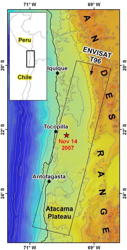
1.3.2 The 2007 Tocopilla Earthquake, Chile
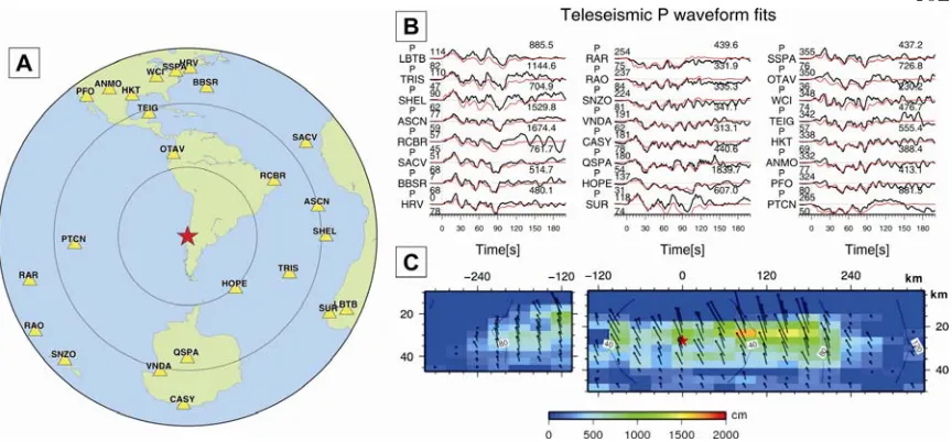
The Mw 7.8 Tocopilla earthquake occurred on 14 November 2007 (15:41 UTC) in northern Chile. The epicenter is located 25 km south of the town of Tocopilla and 150 km north
northeast of the city of Antofagasta (Figure 1.11) [Delouis et al., 2009]. The Global Centroid Moment Tensor (GCMT) catalog solution for the mainshock shows a centroid depth of 38 km and a focal mechanism of a lowangle nodal plane with reverse motion. The solution suggests that this event should be categorized as a subduction underthrusting earthquake occurring at the interface between the subducting Nazca plate and the overriding South American plate. The resultant tectonic signal therefore covers a large area (over 100 km × 500 km).
27
1.12). These two values do not fall into each other’s 95% confidence interval, but this is likely due to the fact that we did not consider the full covariance matrix in our calculation, which is computationally expensive but gives larger and more reasonable values for standard errors [Lohman and Simons, 2005]. After correcting the topographically-correlated tropospheric signals by using these two K values, we clearly see that the phase gradient in the Andes (northern part of the interferogram) is reduced (Figures 1.12b and 1.12e). Compared with the multiscale correction result, the fullinterferogram correlation removes even more of the gradient, but the derived K value is not stable, and in some regions there exists the possibility of overcorrection (Figure 1.12f, near the northeastern corner of the interferogram). In the southernmost part of the interferogram near the Atacama Plateau, the phase increases after applying both corrections. It looks like on the original interferogram, there is positive phasetopography correlation, opposite to the trend in the Andes (Figure 1.12a). However, if we consider the phase change all the way from Antofagasta up to the Atacama Plateau, the phase decreases with elevation. Therefore, the K values derived from both methods are self consistent within the whole interferogram, and the correction result should be valid.
28
length interferogram by using the multiscale approach. Therefore for a given scene, theK value represents the average condition of the vertically stratified troposphere in that given area. Treatment of a system in which K varies slowly in space will be confounded by the effects of convective processes, and is thus not likely to be fruitful.
1.4 Discussion and Conclusions
In the synthetic test, we show that the multiscale approach is insensitive to phase ramps. One important implication of this result is that we can apply this correction before baseline reestimation without confounding the orbital phase ramp with topographicallycorrelated tropospheric signals. When reestimating baseline model parameters from the unwrapped phase and a DEM, largescale differential atmospheric artifacts will be aliased into the baseline estimate [Buckley et al., 2003]. Li et al. [2006a] showed that correcting the interferogram for atmospheric artifacts can effectively improve estimates of baseline parameters. When no satellite imagerybased or modelingbased correction method is available, incorporating a multiscale correction approach can reduce the longwavelength topographicallycorrelated phase to a reasonable extent without overestimating it, allowing more accurate baseline refinement.
30
References of Chapter IBerardino, P., G. Fornaro, R. Lanari, and E. Sansosti (2002), A new algorithm for surface deformation monitoring based on small baseline differential SAR interferograms, IEEE Trans. Geosci. Remote Sens., 40, 2375–2383.
Bevis, M., S. Businger, T. Herring, C. Rocken, R. Anthes, and R. Ware (1992), GPS meteorology: Remote sensing of atmospheric water vapour using the Global Positioning System, J. Geophys. Res., 97, 15787–15801.
Boyd, B., and L. Vandenberghe (2004), Convex Optimization, Cambridge Univ. Press, Cambridge, U. K.
Buckley, S., P. Rosen, S. Hensley, and B. Tapley (2003), Land subsidence in Houston, Texas, measured by radar interferometry and constrained by extensometers, J. Geophys. Res., 108(B11), 2542, doi:10.1029/2002JB001848.
Burgmann, R., P. Rosen, and E. Fielding (2000), Synthetic aperture radar interferometry to measure Earth’s surface topography and its deformation, Annu. Rev. Earth Planet. Sci., 28, 169–209.
Cavalié, O., M.P. Doin, C. Lasserre, and P. Briole (2007), Ground motion measurement in the Lake Mead area, Nevada, by differential synthetic aperture radar interferometry time series analysis: Probing the lithosphere rheological structure, J. Geophys. Res., 112, B03403, doi:10.1029/2006JB004344.
Delacourt, C., P. Briole, and J. Achache (1998), Tropospheric corrections of SAR interferograms with strong topography: Application to Etna, Geophys. Res. Lett., 25, 2849–2852.
Delouis, B., M. Pardo, D. Legrand, and T. Monfret (2009), The Mw 7.7 Tocopilla earthquake of 14 November 2007 at the southern edge of the Northern Chile Seismic Gap: Rupture in the deep part of the coupled plate interface, Bull. Seismol. Soc. Am., 99(1), 87– 94, doi:10.1785/0120080192.
DiCaprio, C., and M. Simons (2008), The importance of ocean tidal load corrections for differential InSAR, Geophys. Res. Lett., 35, L22309, doi:10.1029/2008GL035806.
Doin, M. P., C. Lasserre, G. Peltzer, O. Cavalie, and C. Doubre (2009), Corrections of stratified tropospheric delays in SAR interferometry: Validation with global atmospheric models, J. Appl. Geophys., 69(1), 35–50, doi:10.1016/j.jappgeo.2009.03.010.
Emardson, T., M. Simons, and F. Webb (2003), Neutral atmospheric delay in interferometric synthetic aperture radar applications: Statistical description and mitigation, J. Geophys. Res., 108(B5), 2231, doi:10.1029/2002JB001781.
31
Foster, J., B. Brooks, T. Cherubini, C. Shacat, S. Businger, and C. Werner (2006), Mitigating atmospheric noise for InSAR using a high resolution weather model, Geophys. Res. Lett., 33, L16304, doi:10.1029/2006GL026781.Gray, A. L., K. E. Mattar, and G. Sofko (2000), Influence of ionospheric electron density fluctuations on satellite radar interferometry, Geophys. Res. Lett., 27(10), 1451–1454. Hanssen, R. F. (2001), Radar Interferometry, Data Interpretation and Error Analysis, Springer, New York.
Hill, D., J. Langbein, and S. Prejean (2003), Relations between seismicity and deformation during unrest in Long Valley Caldera, California, from 1995 through 1999, J. Volcanol. Geotherm. Res., 127, 175–193, doi:10.1016/S0377-0273 (03)00169-0.
Ji, C., D. Wald, and D. Helmberger (2002a), Source description of the 1999 Hector Mine, California, earthquake, part I: Wavelet domain inversion theory and resolution analysis,
Bull. Seismol. Soc. Am., 92(4), 1192–1207.
Ji, C., D. Wald, and D. Helmberger (2002b), Source description of the 1999 Hector Mine, California, earthquake, part II: Complexity of slip history, Bull. Seismol. Soc. Am., 92(4), 1208–1226.
Langbein, J. (2003), Deformation of the Long Valley caldera, California: Inferences from measurements from 1988 to 2001, J. Volcanol. Geotherm. Res., 127, 247–267, doi:10.1016/S0377-0273(03)00172-0.
Li, Z., J.P. Muller, and P. Cross (2005), Interferometric synthetic aperture radar (InSAR) atmospheric correction: GPS, Moderate Resolution Imaging Spectroradiometer (MODIS), and InSAR integration, J. Geophys. Res., 110, B03410, doi:10.1029/2004JB003446. Li, Z., E. Fielding, P. Cross, and J.P. Muller (2006a), Interferometric synthetic aperture radar atmospheric correction: GPS topographydependent turbulence model, J. Geophys. Res., 111, B02404, doi:10.1029/2005JB003711.
Li, Z., E. Fielding, P. Cross, and J.P. Muller (2006b), Interferometric synthetic aperture radar atmospheric correction: Medium Resolution Imaging Spectrometer and Advanced Synthetic Aperture Radar integration, Geophys. Res. Lett., 33, L06816, doi:10.1029/2005GL025299.
Li, Z., J.P. Muller, P. Cross, P. Albert, J. Fischer, and R. Bennartz (2006c), Assessment of the potential of MERIS near infrared water vapour products to correct ASAR interferometric measurements, Int. J. Remote Sens., 27, 349–365, doi:10.1080/01431160500307342.
Lohman, R., and M. Simons (2005), Some thoughts on the use of InSAR data to constrain models of surface deformation: Rupture in the deep part of the coupled plate interface,
Bull. Seismol. Soc. Am., 99(1), 87–94, doi:10.1785/0120080192.
32
Meadows, P., B. Rosich, A. Pilgrim, and M. Tranfaglia (2007), ERS2 SAR performance and product evolution, in Proceedings of the Envisat Symposium 2007, Montreux, Switzerland, Eur. Space Agency Spec. Publ., ESA SP636, 23–27.Mogi, K. (1958), Relations between the eruption of various volcanoes and the deformation of the ground surface around them, Bull. Earthquake Res. Inst., 36, 99–143.
Newman, A., T. Dixon, G. Ofoegbu, and J. Dixon (2001), Geodetic and seismic constraints on recent activity at Long Valley Caldera, California: Evidence for viscoelastic rheology, J. Volcanol. Geotherm. Res., 105, 183–206, doi:10.1016/S0377-0273(00)00255-9.
Onn, F., and H. A. Zebker (2006), Correction for interferometric synthetic aperture radar atmospheric phase artifacts using time series of zenith wet delay observations from a GPS network, J. Geophys. Res., 111, B09102, doi:10.1029/2005JB004012.
Puysségur, B., R. Michel, and J.P. Avouac (2007), Tropospheric phase delay in interferometric synthetic aperture radar estimated from meteorological model and multispectral imagery, J. Geophys. Res., 112, B05419, doi:10.1029/2006JB004352.
Simons, M., and P. Rosen (2007), Interferometric synthetic aperture radar geodes, in
Treatise on Geophysics, vol. 3, Geodesy, edited by G. Schubert, pp. 391–446, Elsevier, Amsterdam.
Tichelaar, B. W., and L. J. Ruff (1989), How good are our best models?, Eos Trans. AGU, 70, 593–605.
Zebker, H. A., P. Rosen, and S. Hensley (1997), Atmospheric effects in interferometric synthetic aperture radar surface deformation and topographic maps, J. Geophys. Res., 102, 7547–7563.
33
Table 1.1. Variation of K values with change of scene size in Tocopilla exampleScene Sizea Multiscale FullInterferogram
Full length −0.48 ± 0.01 −1.15 ± 0.03 1/2 length (291–580 km) −0.46 ± 0.02 −0.60 ± 0.14 1/2 length (0–290 km) −0.50 ± 0.04 −2.34 ± 0.11 Average of two 1/2 scenes −0.48 ± 0.04 −1.47 ± 0.18 1/4 length (436–580 km) −0.35 ± 0.02 −1.07 ± 0.01 1/4 length (291–435 km) −1.15 ± 0.02 −1.51 ± 0.05 1/4 length (146–290 km) −0.11 ± 0.04 −19.83 ± 0.19 1/4 length (0–145 km) −0.53 ± 0.02 −0.50 ± 0.01 Average of four 1/4 scenes −0.52 ± 0.05 −5.73 ± 0.20 aFull length: 120 km × 580 km; 1/2 length: 120 km × 290 km; 1/4 length:
34
Figure 1.1. Original and decomposed (top) topography and (middle) interferograms. LP, BP and HP indicate lowpass, bandpass and highpass respectively. The surrounding blank area in each channel results from omitting points along the scene boundaries to avoid edge effects when applying Gaussian filters. (bottom) The scatter plots of each decomposed band. The estimated value of K with uncertainties and correlation coefficient R for each channel are shown at the top right corners of the scatter plots. The final
35
36
37
Figure 1.4. A schematic description of the construction of the synthetic interferometry. (a) The topography of Long Valley Caldera (location is the same as ERS track 485 in Figure 1.3), with maximum elevation (red color) up to ∼4 km. We use the point source model of inflation [Mogi, 1958] to calculate the (b) lineofsight surface displacement due to magmatic intrusion, and use topography to compute (c) topographicallycorrelated tropospheric delays. (d) Turbulent mixing signals and (e) small bilinear ramps are computed as described in the text. We project them to the lineofsight direction and combine them to form the (f) final synthetic interferogram. In this example, for nn is 3
38
39
Figure 1.6. Comparison of decomposed turbulent signals with different scale distance Lc.
40
Figure 1.7. KT time series derived from multiscale approach. We arbitrarily set the first
value in this KT time series as zero, and sequentially add up all KT values. The error bars
41
Figure 1.8. Comparison between observed Kigram, calculated directly from the phase
-topography correlation of each interferogram as shown in equation (2), and estimated
Kigram, derived from the K time series. Outliers are shown in grey circles. These outliers
42
43
Figure 1.10. Scatter plots (phase vs. topography) between two real cases, Long Valley Caldera and Tocopilla, and two synthetic examples. This comparison verifies the high
44
45
46
C h a p t e r 2
PCAIM JOINT INVERSION OF INSAR AND GROUNDBASED GEODETIC TIME SERIES: APPLICATION TO MONITORING MAGMATIC INFLATION BENEATH THE
LONG VALLEY CALDERA
Originally published in Lin, Y.-n. N., A. P. Kositsky, and J.-P. Avouac (2010), PCAIM joint inversion of InSAR and ground-based geodetic time series: Application to monitoring magmatic inflation beneath the Long Valley Caldera, Geophys. Res. Lett., 37(23), L23301, doi: 10.1029/2010GL045769.
Abstract
This study demonstrates the interest of using a Principal Component Analysisbased Inversion Method (PCAIM) to analyze jointly InSAR and groundbased geodetic time series of crustal deformation. A major advantage of this approach is that the InSAR tropospheric biases are naturally filtered out provided they do not introduce correlated or high amplitude noise in the input times series. This approach yields source models which are wellconstrained both in time and space due to the temporal resolution of the ground
47
the performance of this approach, we apply it to the 1997–98 magmatic inflation event in the Long Valley Caldera, California.2. 1 Introduction
A number of groundbased geodetic techniques and remote sensing techniques are now available to monitor surface deformation induced by a variety of geophysical processes and are used to address a wide range of questions in various fields [e.g., Blewitt, 2007; Simons and Rosen, 2007]. Some groundbased geodetic techniques, such as Electronic Distance Meter (EDM) and Global Positioning System (GPS), allow high temporal resolution, with sampling rates typically between more than 1 measurement epoch per second and 1 measurement epoch every several days. These measurements are based on electromagnetic signals transmitted through the atmosphere between pairs of ground
based stations or between groundbased stations and satellites, and are therefore sensitive to atmospheric effects. Atmospheric effects are routinely estimated and corrected for in processing continuous GPS data [Tregoning and Herring, 2006; Blewitt, 2007] and EDM data [Langbein et al., 1987]. Therefore, such postcorrected time series are relatively free of atmospheric bias.
48
moisture variations in the troposphere. Various methods have been proposed to correct these effects [e.g., Li et al., 2005, 2006; Foster et al., 2006; Onn and Zebker, 2006;Puysségur et al., 2007; Doin et al., 2009; Lin et al., 2010], but the potential of these techniques is limited by the availability of radiometric data, the density of GPS stations, or the accuracy of highresolution weather models. Difficulties in correcting atmospheric influences, in addition to the generally long time span between interferometric pairs of images, strongly limit the possibility of using InSAR to monitor the temporal variation of surface deformation.
49
in terms of spatiotemporal sampling rates in the PCAIM output. In this study, we use the Long Valley Caldera example to test this joint inversion method. Long Valley Caldera experienced a large inflation episode between 1997 and 1998, resulting in ∼10 cm of cumulative uplift [Langbein, 2003]. Hereafter we show how to derive a source model with high spatiotemporal resolution from the joint inversion of InSAR and groundbased geodetic data.2. 2 Joint Inversion Using PCAIM
2.2.1 PCAIM Principles
50
spatial function is modeled individually and translated into a corresponding principal source model. The various principal source models are then recombined with their respective principal values and time functions to represent the estimate of the source model needed to fit the original dataset. PCAIM thus takes advantage of the linearity of the formulation and is cost effective because it generally requires inversion of only a handful of spatial components. For more details regarding the theoretical and technical aspects of this method, the reader can refer to Kositsky and Avouac [2010].2.2.2 PCA Decomposition
51
than the standard PCA technique when the time series have missing data and/or varying uncertainties [Kositsky and Avouac, 2010].Another adaptation is that each component is solved separately in order to preserve the continuity of time functions. This iterative decomposition strategy retains the signal continuity of each component (Appendix A). The resultant principal components are close to but not exactly orthogonal. Nevertheless, orthogonality is not geophy