University of Windsor University of Windsor
Scholarship at UWindsor
Scholarship at UWindsor
Electronic Theses and Dissertations Theses, Dissertations, and Major Papers
9-20-2018
Multi-Objective Drive-Cycle Based Design Optimization of
Multi-Objective Drive-Cycle Based Design Optimization of
Permanent Magnet Synchronous Machines
Permanent Magnet Synchronous Machines
Philip Korta
University of Windsor
Follow this and additional works at: https://scholar.uwindsor.ca/etd
Recommended Citation Recommended Citation
Korta, Philip, "Multi-Objective Drive-Cycle Based Design Optimization of Permanent Magnet Synchronous Machines" (2018). Electronic Theses and Dissertations. 7535.
https://scholar.uwindsor.ca/etd/7535
This online database contains the full-text of PhD dissertations and Masters’ theses of University of Windsor students from 1954 forward. These documents are made available for personal study and research purposes only, in accordance with the Canadian Copyright Act and the Creative Commons license—CC BY-NC-ND (Attribution, Non-Commercial, No Derivative Works). Under this license, works must always be attributed to the copyright holder (original author), cannot be used for any commercial purposes, and may not be altered. Any other use would require the permission of the copyright holder. Students may inquire about withdrawing their dissertation and/or thesis from this database. For additional inquiries, please contact the repository administrator via email
Multi-Objective Drive-Cycle Based
Design Optimization of Permanent
Magnet Synchronous Machines
By
Philip Korta
A Thesis
Submitted to the Faculty of Graduate Studies through the Department of Electrical and Computer Engineering in Partial
Fulfillment of the Requirements for the Degree of Master of Applied Science at the University of Windsor
Windsor, Ontario, Canada
2018
Multi-Objective Drive-Cycle Based Design Optimization of Permanent Magnet Synchronous Machines
by
Philip Korta
APPROVED BY:
______________________________________________ B. Minaker
Department of Mechanical, Automotive & Materials Engineering
______________________________________________ B. Balasingam
Department of Electrical and Computer Engineering
______________________________________________ N. C. Kar, Advisor
Department of Electrical and Computer Engineering
iii
DECLARATION OF ORIGINALITY
I hereby certify that I am the sole author of this thesis and that no part of this thesis has been published or submitted for publication.
I certify that, to the best of my knowledge, my thesis does not infringe upon anyone’s copyright nor violate any proprietary rights and that any ideas, techniques, quotations, or any other material from the work of other people included in my thesis, published or otherwise, are fully acknowledged in accordance with the standard referencing practices. Furthermore, to the extent that I have included copyrighted material that surpasses the bounds of fair dealing within the meaning of the Canada Copyright Act, I certify that I have obtained a written permission from the copyright owner(s) to include such material(s) in my thesis and have included copies of such copyright clearances to my appendix.
iv ABSTRACT
Research conducted previously has shown that a battery electric vehicle (BEV) motor design incorporating drive-cycle optimization can lead to achievement of a higher torque density motor that consumes less energy over the drive-cycle in comparison to a conventionally designed motor. Such a motor indirectly extends the driving range of the BEV. Firstly, in this thesis, a vehicle dynamics model for a direct-drive machine and its associated vehicle parameters is implemented for the urban dynamometer driving schedule (UDDS) to derive loading data in terms of torque, speed, power, and energy. K-means clustering and Gaussian mixture modeling (GMM) are two clustering techniques used to reduce the number of machine operating points of the drive-cycle while preserving the characteristics of the entire cycle. These methods offer high computational efficiency and low computational time cost while optimizing an electric machine. Differential evolution (DE) is employed to optimize the baseline fractional slot concentrated winding (FSCW) surface permanent magnet synchronous machine (SPMSM). A computationally efficient finite element analysis (CEFEA) technique is developed to evaluate the machine at the representative drive-cycle points elicited from the clustering approaches. In addition, a steady-state thermal model is established to assess the electric motor temperature variation between optimization design candidates.
v
ACKNOWLEDGEMENTS
Firstly, I would like to thank my supervisor, Dr. Narayan Kar who guided me into and supported me throughout the master’s program. He recognized my potential and gave me all the tools necessary to become an exceptional researcher. In addition, he provided me with an abundant amount of opportunities to attend technical conferences and meet with industries to gain confidence and help me grow as a professional in the field of electric vehicle applications.
I would like to thank Dr. Balakumar Balasingam who took the time to sit with me and have technical discussions. He provided me with many insights in the field of machine learning and clustering techniques. I would also like to acknowledge Dr. Bruce Minaker who provided me with feedback and motivated me to incorporate thermal analysis into my work.
I would also like to sincerely thank Dr. Lakshmi Varaha Iyer who mentored me throughout my master’s program and guided me towards my research topics. He provided me with opportunities to work on novel and interesting topics and pushed me to accomplish things that I am proud of and would have never achieved otherwise.
vi
TABLE OF CONTENTS
DECLARATION OF ORIGINALITY ... iii
ABSTRACT ... iv
ACKNOWLEDGEMENTS ... v
LIST OF TABLES ... ix
LIST OF FIGURES ... xi
LIST OF ABBREVIATIONS/SYMBOLS ... xiv
NOMENCLATURE ... xv
CHAPTER 1 Introduction... 1
1.1 Objectives and Contributions of This Study ... 2
1.2 Organization of Thesis ... 3
CHAPTER 2 Vehicle Dynamics for Drive-Cycle Operating Characteristics... 5
2.1 Drive-Cycles ... 5
2.2 Vehicle Parameters ... 6
2.3 Deriving Motor Load Characteristics with Vehicle Dynamics Model ... 7
2.3.1 Motor Output Torque for UDDS Drive-Cycle ... 9
2.3.2 Motor Speed for UDDS Drive-Cycle ... 11
2.3.3 Motor Output Power for UDDS Drive-Cycle... 11
2.3.4 Motor Energy Distribution on the Torque-Speed plane ... 12
2.4 Conclusions ... 13
CHAPTER 3 Clustering Techniques for Drive-Cycle Data Representation ... 15
3.1 K-Means Clustering ... 15
3.2 Selecting Number of Clusters in K-Means ... 16
3.2.1 Sum of Squared Error Analysis ... 17
3.3 Addressing Energy Significance in Clustering Algorithms ... 17
3.3.1 Hybrid Clustering Technique ... 18
3.3.2 Results for Hybrid Clustering Technique ... 19
3.3.3 Data Resampling Technique ... 20
3.3.4 Results for Data Resampling Technique ... 20
vii
3.4.1 Expectation Maximization Algorithm ... 23
3.4.2 MMDL for Component Selection in GMM... 25
3.4.3Results for GMM using Resampling Technique ... 25
3.5 Conclusions ... 27
CHAPTER 4 Computationally Efficient FEA Machine Evaluation Procedure... 29
4.1 Baseline Machine for Analysis ... 29
4.2 Computationally Efficient Finite Element Analysis ... 33
4.2.1 Electric Symmetry of PMSMs ... 33
4.2.2 Flux-Linkage, Back EMF, and Torque Derivation ... 36
4.3 Scaling Stack Length for Desired Torque Production ... 38
4.4 Current Selection for Accurate Load Analysis ... 40
4.5 Loss Analysis ... 44
4.5.1 Copper Loss ... 44
4.5.2 Core Loss ... 44
4.5.3 Mechanical Loss ... 45
4.5.4 Efficiency Calculation ... 46
4.6 Weight and Component Cost Calculation ... 47
4.7 Conclusions ... 48
CHAPTER 5 Steady-State Thermal Analysis of Electric Machines ... 50
5.1 Modes of Heat Transfer ... 50
5.1.1 Thermal Conduction ... 50
5.1.2 Thermal Convection ... 51
5.1.3 Thermal Radiation ... 51
5.2 Lumped Parameter Thermal Network ... 51
5.2.1 Thermal Resistance ... 52
5.2.2 Thermal Capacitance ... 52
5.2.3 Thermal Sources ... 53
5.3 Steady-State Temperature Analysis of Electric Machines ... 53
5.4 Conclusions ... 57
CHAPTER 6 Multi-Objective Drive-Cycle Based Optimization ... 58
viii
6.1.1 Initial Population ... 58
6.1.2 Creation of Trial Design Candidates... 59
6.1.3 Logical Dominance Function ... 60
6.1.4 Termination Condition ... 60
6.2 Optimization Parameters, Constraints, and Objectives ... 60
6.3 Optimization Results ... 63
6.4 Conclusions ... 68
CHAPTER 7 Drive-Cycle Analysis of Inverter Fed Machines ... 69
7.1 UDDS Drive-Cycle Vehicle Loading Analysis ... 72
7.2 Motor Current Selection and Inductance Parameter Determination ... 77
7.3 PSIM Motor Drive Simulation... 80
7.4 FEA Motor Analysis of Time Harmonic Effects ... 86
7.5 Conclusions ... 92
CHAPTER 8 Conclusions... 93
8.1 Future Work ... 94
REFERENCES/BIBLIOGRAPHY ... 95
APPENDICES ... 100
Appendix A. Permission for using IEEE Publications ... 100
ix
LIST OF TABLES
TABLE 2.1 2014 Ford Fiesta Specifications ... 8
TABLE 3.1 Hybrid Clustering Result ... 20
TABLE 3.2 K-Means Clustering Result for Resampled Data ... 21
TABLE 3.3 Gaussian Mixture Modeling Result for Resampled Data ... 27
TABLE 4.1. Design Targets for Direct-Drive FSCW SPMSM ... 30
TABLE 4.2 Stator Design Details of the Direct-Drive Machine ... 32
TABLE 4.3 Rotor Design Details of the Direct-Drive Machine ... 32
TABLE 4.4 Slot Design Details of the Direct-Drive Machine ... 33
TABLE 4.5 Density of Materials used in the Direct-Drive Machine... 47
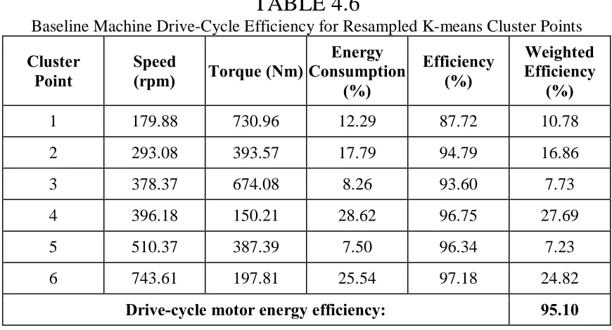
TABLE 4.6 Baseline Machine Drive-Cycle Efficiency for Resampled K-means Cluster Points ... 48
TABLE 5.1 Thermal Conductivity of Components in the Direct-Drive Machine... 56
TABLE 5.2 Steady-State Temperature Results of the Direct-Drive Machine at Various Load Conditions ... 57
TABLE 6.1 Optimization Parameters and Limits ... 63
TABLE 6.2 K-means Results for Maximized Objectives ... 66
TABLE 6.3 GMM Results for Maximized Objectives... 66
TABLE 6.4 Drive-Cycle Energy Efficiency Derived From Representative Load Points 67 TABLE 6.5 Optimized Motor Parameters for Drive-Cycle Efficiency... 67
TABLE 7.1 Motor Specifications for Inverter Simulation ... 72
TABLE 7.2 Vehicle Specifications ... 73
TABLE 7.3 K-Means Clustering Result for Resampled Data ... 76
TABLE 7.4 K-Means Clustering Result and Associated Motor Parameters ... 79
TABLE 7.5 IGBT and GaN Specifications ... 81
TABLE 7.6 IGBT and GaN Torque Ripple Comparison ... 88
TABLE 7.7 IGBT and GaN Stranded Loss Comparison ... 90
TABLE 7.8 IGBT and GaN Core Loss Comparison ... 90
TABLE 7.9 IGBT and GaN Solid Loss Comparison ... 90
x
xi
LIST OF FIGURES
Figure 1.1 Torque-speed and power-speed characteristics of a typical PMSM ... 2
Figure 2.1 Urban Dynamometer Driving Schedule (UDDS) ... 7
Figure 2.2 Highway Fuel Economy Driving Schedule (HWFET) ... 7
Figure 2.3 UDDS resultant vehicle force for 2014 Ford Fiesta ... 8
Figure 2.4 Relationship between vehicle force and output torque ... 9
Figure 2.5 Driveline components of a typical electric vehicle ... 10
Figure 2.6 UDDS torque profile for a direct-drive machine ... 11
Figure 2.7 UDDS motor speed in rpm for a direct-drive machine ... 12
Figure 2.8 UDDS output power profile ... 12
Figure 2.9 UDDS torque-speed load characteristics for direct-drive machine ... 13
Figure 2.10 UDDS energy distribution across the torque-speed plane for a direct-drive machine ... 14
Figure 3.1 K-means clustering result for torque-speed load data ... 16
Figure 3.2 Sum of squared error results for cluster selection ... 17
Figure 3.3 Results for hybrid clustering approach ... 19
Figure 3.4 Results for K-means clustering using the resampled dataset ... 21
Figure 3.5 Normal distributions with varying means and covariance ... 22
Figure 3.6 Mixture model of normal distributions ... 22
Figure 3.7 Mixture minimum description length for component selection ... 26
Figure 3.8 Gaussian mixture modeling result for resampled dataset ... 26
Figure 4.1 Cross-section of 36/30 direct-drive baseline machine ... 31
Figure 4.2 Torque-speed and power-speed characteristics of the baseline direct-drive FSCW SPMSM ... 31
Figure 4.3 Three phase flux-linkage waveform results obtained from five magnetostatic solutions ... 34
Figure 4.4 30 samples of the phase A flux-linkage waveform obtained from five magnetostatic solutions ... 34
Figure 4.5 Coil around tooth and virtual coil around stator back iron used in FEA ... 35
xii
Figure 4.7 Flux-linkage waveform derived from FEA ... 37
Figure 4.8 Back EMF waveform derived from FEA ... 38
Figure 4.9 Continuous torque waveform derived from FEA ... 38
Figure 4.10 d- and q-axis flux-linkages determined from 3-phase flux-linkage waveforms ... 40
Figure 4.11 d-axis flux-linkage map for varying d- and q-axis excitations ... 42
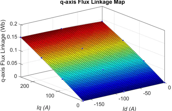
Figure 4.12 q-axis flux-linkage map for varying d- and q-axis excitations ... 42
Figure 4.13 Torque map for varying d- and q-axis excitations ... 43
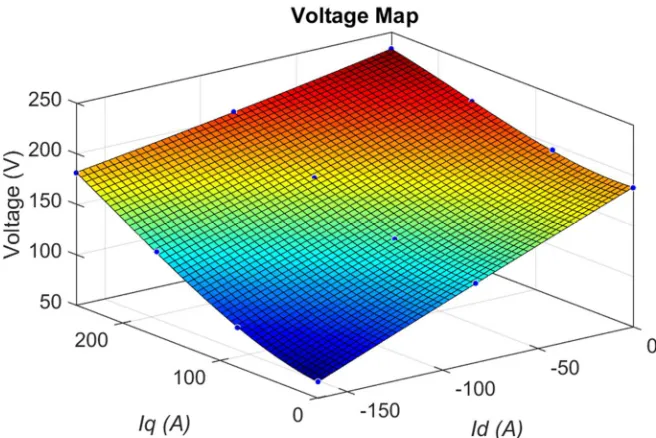
Figure 4.14 Voltage map for varying d- and q-axis excitations ... 43
Figure 4.15 Stator tooth flux density ... 46
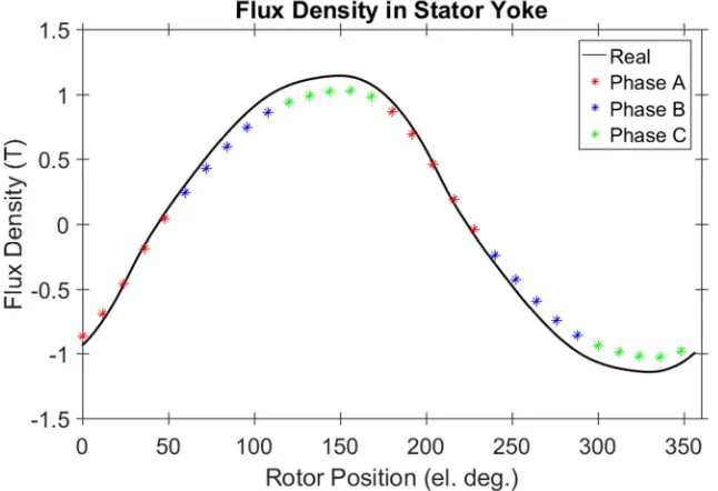
Figure 4.16 Stator yoke flux density ... 46
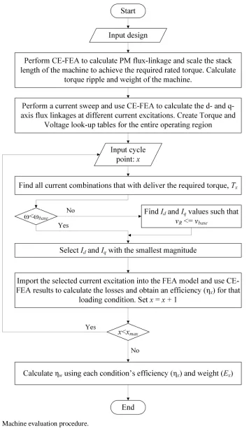
Figure 4.17 Machine evaluation procedure ... 49
Figure 5.1 Heat flow path for copper losses in an electric machine ... 54
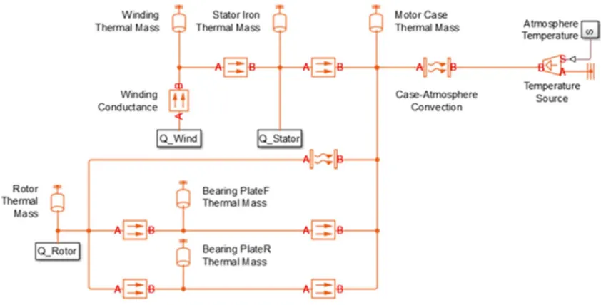
Figure 5.2 LPTN Simulink model of an electric motor ... 54
Figure 5.3 Thermal circuit of an electric machine ... 55
Figure 5.4 Steady-state thermal circuit of an electric machine ... 56
Figure 6.1 Multi-objective differential evolution flowchart ... 61
Figure 6.2 Optimization parameters selected for baseline machine ... 62
Figure 6.3 Optimization results using the resampled K-means clustering drive-cycle points... 65
Figure 6.4 FEA waveforms displaying torque ripple of baseline and optimized machine. ... 66
Figure 7.1 PWM gate pulses generated by comparing a triangular carrier wave with the desired waveform ... 69
Figure 7.2 Typical configuration of a two-level inverter ... 70
Figure 7.3 Flowchart for IGBT and GaN comparison on motor performance ... 71
Figure 7.4 Cross-section of 12/14 SPM used for the system level investigation ... 72
Figure 7.5 UDDS motor speed obtained for 12/14 SPM ... 74
Figure 7.6 UDDS motor torque obtained for 12/14 SPM ... 74
Figure 7.7 UDDS output power obtained for 12/14 SPM ... 75
xiii
Figure 7.9 K-means clustering result on the resampled dataset of the 12/14 SPM
torque-speed load distribution ... 76
Figure 7.10 Efficiency map of the 12/14 SPM ... 77
Figure 7.11 Variation of Id in the torque-speed plane ... 78
Figure 7.12 Variation of Iq in the torque-speed plane ... 78
Figure 7.13 Variation of Ld in the torque-speed plane ... 79
Figure 7.14 Variation of Lq in the torque-speed plane ... 80
Figure 7.15 Current control diagram for inverter-motor simulation ... 81
Figure 7.16 PSIM schematic of two-level IGBT inverter ... 82
Figure 7.17 PSIM schematic of two-level GaN inverter ... 83
Figure 7.18 PSIM results for the first cluster point of the IGBT simulation ... 85
Figure 7.19 Three-phase current excitation exported from PSIM ... 86
Figure 7.20 Current excitation comparison for the first cluster point of ideal, IGBT, and GaN simulations ... 87
Figure 7.21 Torque comparison for the first cluster point of ideal, IGBT, and GaN simulations ... 87
Figure 7.22 Stranded loss comparison for the first cluster point of ideal, IGBT, and GaN simulations ... 88
Figure 7.23 Core loss comparison for the first cluster point of ideal, IGBT, and GaN simulations ... 89
xiv
LIST OF ABBREVIATIONS/SYMBOLS
BEV Battery Electric Vehicle
DE Differential Evolution
PMSM Permanent Magnet Synchronous Machine
FEA Finite Element Analysis
LPTN Lumped Parameter Thermal Network
GaN Gallium Nitride
IGBT Insulated-Gate Bipolar Transistor
EV Electric Vehicle
EPA Environmental Protection Agency
UDDS Urban Dynamometer Driving Schedule
HWFET Highway Fuel Economy Driving Schedule
SSE Sum of Squared Error
ECG Energy Center of Gravity
GMM Gaussian Mixture Modeling
EM Expectation Maximization
MMDL Mixture Minimum Description Length
CEFEA Computationally Efficient Finite Element Analysis
FSCW Fractional Slot Concentrated Winding
SPMSM Surface Permanent Magnet Synchronous Machine
MTPA Maximum Torque per Ampere
FW Field/Flux Weakening
FEM Finite Element Method
FFT Fast Fourier Transform
xv
NOMENCLATURE
FD Drag force
FR Tire friction force
FA Force of acceleration
FG Gravitational force
Fv Resultant vehicle force
ρ Chapter 2: Density of air
Chapter 4: Resistivity of copper
Cd Drag coefficient
Av Frontal vehicle surface area
frr Coefficient of rolling resistance
Mv Vehicle mass
v Chapter 2: Speed in m/s
Chapter 4: Harmonic order
g Gravitational acceleration
α Chapter 2: Road grade
Chapter 3: Mixing probability or component distribution
r Wheel radius
ig Gear ratio
T Chapter 2: Torque
Chapter 7: PI time constant
η Efficiency
N Speed in rpm
P Chapter 2: Power
Chapter 4: Number of poles
Chapter 6: Parent Chapter 7: PI gain
ω Chapter 2: Speed in rad/sec
Chapter 4: Specific core loss
E Energy
xvi
m Chapter 3: Cluster’s mean in K-means
Chapter 4: Mass
µ Gaussian mean
σ2
Covariance
C Covariance matrix
θ Chapter 3: Parameter vector of a given component (µm,Cm)
Chapter 4: Phase angle
Chapter 5: Temperature
Θ(K) Parameter set defining a given mixture
δµ Stopping condition tolerance for Gaussian mean
δC Stopping condition tolerance for Gaussian covariance matrix
A Chapter 4: Magnetic vector potential
Chapter 5: Isothermal surface area perpendicular to the direction of heat flow
Φ Radial flux per unit axial length for one turn of a coil placed around a
stator tooth
λ Flux linkage
ϕv Harmonic phase angle
ea Back EMF
I Current excitation
L Motor length
V Voltage
J Current density
PCu Copper loss
B Flux density
tw Tooth width
yw Yoke width
kh Hysteresis loss coefficient
ke Eddy-current loss coefficient
f Frequency
xvii Pmech Mechanical loss
kf Viscous friction coefficient
cm Material cost index
H Quantity of heat transferred
q Heat transfer rate
k Thermal conductivity of a medium
x Direction of heat flow
h Convective heat transfer coefficient
σ Stefan-Boltzmann
ε Emissivity of a body
Rth Thermal resistance
cp Specific heat capacity
Cth Thermal capacitance
bjU, bjL Upper and lower bounds of a design parameter
F Mutation intensity
Cr Crossover probability
c Child
Tcoil Turns per coil
Dro Rotor outer diameter
Wt Tooth width
Wso Slot opening width
αPM Magnet angle
fsw Switching frequency
1
CHAPTER 1
Introduction
Electric vehicles have captured a vast amount of attention in the past decade due to environmental concerns from fossil fuel emissions and the public’s desire for innovation. Furthermore, auto manufacturers must meet government regulations to meet strict fuel efficiencies targets in next-generation vehicles [1], [2]. Permanent magnet synchronous machines (PMSMs) are currently leading the competition amongst other types of electric motors to replace the standard internal combustion engine due to their high power density and efficiency [3]. However, even as the most suitable electric machine, there is still opportunity to improve in areas of reliability, losses, temperature, size, cost, and active weight [4]. This is evident by the electric vehicle’s requirements to be efficient over a wide speed operating range to obtain increased driving distance on a single battery charge and for the vehicle to be affordable for the mass population [5].
2
Fig. 1.1. Torque-speed and power-speed characteristics of a typical PMSM.
Although electric motors have been around for over a century, their use in traction applications for electric vehicles remains a modern and developing application that still requires a significant amount of research and development in terms of weight, cost, size, efficiency, reliability, and power density of the electric motor. This requires careful analysis of the electric vehicle to optimally design the electric motor for the specific application.
1.1 Objectives and Contributions of This Study
In electric motor design optimization procedures, the objective has commonly been to maximize the motor efficiency at rated conditions due to the computational demand of finite element analysis as in [9]. However, in a practical vehicle application, the motor performs at various torque and speed operating conditions while driving [10]. A PMSM is not able to deliver the peak efficiency across the entire operating range. Therefore, a new motor design procedure is required to evaluate machine performance across a wide range of operating conditions. This will ensure that an electric motor will perform with optimal efficiency in a practical vehicle application where it is subject to various torque and speed loading conditions.
3
harmonics, cause an increase in torque ripple and vibrations as well as additional harmonic losses [11]. Therefore, it is essential to model the inverter excitations that include harmonics to assess the negative effects that they have on the motor. Moreover, drive-cycle analysis is required to accurately evaluate the overall machine performance in a system that is prevalent in real driving conditions.
This thesis proposes modeling for torque, speed, and power characterization of the electric motor in a vehicle application. The vast amount of derived drive-cycle load points requires quantization by means of clustering or mixture modeling to make drive-cycle analysis computationally feasible by representing the entire drive-cycle with a minimal number of load points.
Further, the thesis proposes a method to optimize an electric machine for this set of torque-speed load points that are most crucial for a given vehicle when executing a selected drive-cycle. This ensures that optimal motor energy efficiency will be obtained in a practical vehicle application. Additionally, a thermal analysis is included into the
optimization to consider temperature variations in different motor topologies. Thereafter,
to analyze the electric motor on a system level drive-cycle analysis, a performance comparison is introduced to rival the effects that different inverters have on an electric motor in terms of torque ripple and drive-cycle energy efficiency.
1.2 Organization of Thesis
Chapter 2 utilizes vehicle dynamic equations to analyze the forces experienced by a particular vehicle whilst performing a drive-cycle to derive torque, speed, and energy distribution experienced by the electric machine.
Chapter 3 focuses to reduce the computational burden that this vast amount of loading data contains by implementing machine learning algorithms such as K-means clustering and Gaussian mixture modeling to cluster and quantize the data. This will in turn produce a reduced number of representative points that retain the loading characteristics experienced by the machine across the drive-cycle.
4
efficient and accurate performance characteristics. This technique enables the continuous torque, back EMF, and flux density waveforms to be derived that contain nonlinearities such as harmonics and saturation by combining a limited number of FEA solutions with Fourier analysis to reconstruct the continuous waveforms. These characteristics are used in a loss model developed to determine the machine efficiency at a given operating condition.
Chapter 5 outlines the procedure for constructing a lumped parameter thermal network (LPTN) to analyze the temperatures of the machine at different locations in the motor structure. The model uses the losses calculated in Chapter 4 to determine the steady-state operating temperatures of the machine in different load conditions.
Chapter 6 introduces a multi-objective differential evolution optimization program that creates machine design candidates and evaluates the designs based on their performance across the drive-cycle representative load points. The evolutionary algorithm modifies the geometrical structure of the machine and converges to uncover models that are optimal in terms of cost, weight, torque ripple, and efficiency across the drive-cycle points. This ensures that the vehicle will operate with the lowest amount of energy consumption possible while satisfying stringent constraints on weight and torque ripple production.
Chapter 7 extends the research work to the system level by analyzing the effects of inverter-generated harmonics on an electric motor. Gallium nitride (GaN) and insulated-gate bipolar (IGBT) two-level inverter system simulations are created to obtain the current excitations with harmonic content at drive-cycle representative load points. FEA is used to analyze the inverter harmonic effects on the torque ripple and losses of the machine. A drive-cycle comparison of the GaN and IGBT inverter topologies with analytically calculated pure sinusoidal waveforms is conducted.
5
CHAPTER 2
Vehicle Dynamics for Drive-Cycle Operating Characteristics
Vehicle dynamic simulations provide essential information to understand the torque and speed requirements of a motor while subject to different driving conditions [12]. The vehicle dynamic equations listed in (2.1) – (2.4) analyze the forces that act on a vehicle in motion. The main forces can be analytically represented by the drag force associated with the aerodynamics of the vehicle and the extent of wind resistance the vehicle is experiencing, the static and dynamic tire friction force, the force of acceleration that is associated with the vehicle’s inertia, and the gravitational force that the vehicle experiences when there is a road grade present. The sum of these four forces describes the overall resultant force acting on the vehicle, expressed in (2.5) [13].
2
1 2
D d v
F = r C A v (2.1)
cos
R rr v
F = f M g a (2.2)
A v dv F M dt = (2.3) sin G v
F =M g a (2.4)
v D R A G
F =F +F +F +F (2.5)
where ρ is the density of air, Cd is the drag coefficient, Av is the frontal vehicle surface area, v is the vehicle speed, frr is the coefficient of rolling resistance, Mv is the vehicle
mass, g is gravitational acceleration, and α is the road grade.
2.1 Drive-Cycles
Drive cycles are a series of data points that contain vehicle speed versus time. They are created to simulate real-life driving conditions and are most often used for performance assessment of an automobile in terms of vehicle mileage and emissions. Electric vehicles
(EVs) do not generate emissions, but vehicle mileage is one of the principle design
6
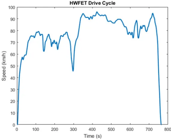
The Environmental Protection Agency (EPA) developed the Urban Dynamometer Driving Schedule (UDDS) to simulate city driving and the Highway Fuel Economy Driving Schedule (HWFET) for highway driving [14]. Many other corporations and countries have various drive-cycles to represent common driving conditions as well as aggressive driving styles present in high traffic situations. They are used as a baseline for vehicle performance during prototype development to predict product functionality and lifespan once the vehicle enters the market. It is therefore essential that vehicle components be designed to withstand and perform most efficiently on suitable drive-cycles for specific vehicle applications. For this reason, the aforementioned vehicle dynamics are applied to a drive-cycle to analyze the forces acting on the vehicle and predict design targets, such as torque and speed requirements, to develop optimally efficient products for specific vehicle applications.
The UDDS and HWFET obtained from [14] are the standard tests conducted in Canada for city and highway evaluation of cars and light trucks. This thesis will focus specifically on the UDDS cycle to have a practical design target for vehicles in production in this area. The urban cycle displayed in Fig. 2.1 experiences a lower average speed of 34.1 km/h and 23 full stops. The cycle covers a total distance of 17.77 km over a duration of 1,874 seconds. The highway drive-cycle displayed in Fig. 2.2 has a higher average speed of 77.7 km/h, covering a total distance of 16.45 km, with a duration of 765 seconds [15].
2.2 Vehicle Parameters
In order to acquire machine design targets and analyze the loading conditions that the electric motor is subject to, vehicle parameters are required for which the electric motor will be integrated into. These vehicle parameters include the drag coefficient, frontal
vehicle surface area, rolling resistance coefficient, vehicle mass, and wheel radius rw.
7 Fig. 2.1. Urban Dynamometer Driving Schedule (UDDS).
Fig. 2.2. Highway Fuel Economy Driving Schedule (HWFET).
2.3 Deriving Motor Load Characteristics with Vehicle Dynamics Model
The resultant vehicle force in (2.5) is obtained by calculating the individual forces at each
8
TABLE 2.1
2014 Ford Fiesta Specifications
Symbol Description Value
ρ Density of air 1.202 kg/m3
Cd Drag coefficient 0.33
Av Frontal vehicle surface area 2.536 m2
v Vehicle speed varying
frr Rolling resistance
coefficient 0.013
Mv Vehicle mass 1,570 kg
g Gravitational acceleration 9.81 m/s2
α Road grade 0°
rw Wheel Radius (195/50R16) 0.3007 m
ig Gear Ratio 1
9
2.3.1 Motor Output Torque for UDDS Drive-Cycle
The vehicle force is applied at the wheel of the vehicle to drive the vehicle. However, the focus of this thesis is the motor, and thus, the resultant vehicle force must be translated back and converted into the output speed and torque of the electric motor. Equation (2.6) uses the resultant vehicle force and the moment arm of the wheel, shown in Fig. 2.4, to
derive the torque Tw at the shaft of the vehicle [12].
w v w
T = F r (2.6)
Fig. 2.4. Relationship between vehicle force and output torque.
The transmission system of an electric vehicle often includes a fixed gear ratio between the motor and the output shaft. This gear ratio is used to scale-down the amount of torque
production and increase the speed required of the electric motor. The motor torque Tp is
related to the torque at the wheel Tw as in (2.7) where ig is the gear ratio and η is the driveline efficiency [12]. The driveline efficiency includes all losses associated with the gears and the differential. A transmission system contributes losses that account for 2 – 20% of the total output power in the vehicle depending on the operating speed and torque [17], [18]. Figure 2.5 illustrates the configuration of driveline components in a typical electric vehicle.
w p
g
T T
i
=
10 Fig. 2.5. Driveline components of a typical electric vehicle.
11 Fig. 2.6. UDDS torque profile for a direct-drive machine.
2.3.2 Motor Speed for UDDS Drive-Cycle
In addition, the output motor speed, Np, is a function of the gear ratio and the wheel
speed, Nw, as seen in (2.8). The wheel speed is converted from kilometers per hour to
revolutions per minute using (2.9). Figure 2.7 displays the speed of the motor’s rotor in revolutions per minute (rpm) [12].
p g w
N =i N (2.8)
30
w w
r v N =
p (2.9)
2.3.3 Motor Output Power for UDDS Drive-Cycle
The product of torque and speed in radians per second, ω, defines the instantaneous output power, Pout, of the electric motor as seen in (2.10) [13]. Figure 2.8 displays this characteristic across the urban drive-cycle. Similar to the torque profile, positive power flow denotes motoring and the negative regions display the magnitude of power that is available for regenerative braking. In this thesis, the electric machine is being analyzed for the motoring condition and only considers the positive torque and power regions.
out
12 Fig. 2.7. UDDS motor speed in rpm for a direct-drive machine.
5
Fig. 2.8. UDDS output power profile.
2.3.4 Motor Energy Distribution on the Torque-Speed plane
13
Fig. 2.9. UDDS torque-speed load characteristics for direct-drive machine.
Another significant characteristic of the loading conditions is their associated energy consumption. This is an important characteristic because the motor design must be optimally efficient in regions with high energy consumption to reduce the amount of battery consumption in driving scenarios [13].
Energy is defined as the integral of power over time and can be represented as (2.11)
where the motor energy, Emotor, is equal to the summation of the discrete samples of
power. Similarly, the energy associated with each load point on the torque-speed plane can be calculated using the number of occurrences of that condition in the drive-cycle multiplied by its associated power [13]. The overall energy distribution across the torque-speed plane is shown in Fig. 2.10.
( )
0
t motor out
t
E P t
=
=
å
(2.11)2.4 Conclusions
14
Fig. 2.10. UDDS energy distribution across the torque-speed plane for a direct-drive machine.
consumption. This torque-speed distribution can be used to assist in selecting a machine’s operating envelope when designing a machine by identifying maximum torque and speed requirements of the motor. Furthermore, regions with a high density of points and points with large magnitudes of energy consumption can be identified and targeted in the
machine design process to ensure maximum drive-cycle operating efficiency. The regions with a high density of load points are produced when the vehicle is operating frequently around a target speed limit such as 50 km/h for city and 100 km/h for highway. Load points that have a large magnitude of energy consumption are caused by a number of repetitive occurrences and large value of instantaneous power.
It was found that regions of acceleration experience a high torque, but low speed for a short duration of time, therefore the magnitude of energy consumption during
15
CHAPTER 3
Clustering Techniques for Drive-Cycle Data Representation
To properly assess a machine’s performance across a drive-cycle, the motor’s efficiency must be determined at each load point on the torque-speed plane. However, this is computationally intensive due to the vast amount of individual sample points. Thus, statistical data-mining algorithms are introduced to quantize the load data into a minimal number of points that preserve and represent the characteristics of the full dataset. This creates a computationally efficient method of evaluating a machine’s performance across an entire drive-cycle and makes it feasible to implement this type of machine evaluation into an optimization algorithm [21].
3.1 K-Means Clustering
K-means clustering is a statistical algorithm proposed in [22] for drive-cycle data
representation. The algorithm separates the data points into K clusters where each data
point belongs to the cluster with the nearest mean. In an iterative process, the data points get assigned to the nearest mean and the new mean for each cluster is recalculated once all the assignments are complete.
The user defines the number of desired clusters by assigning random points in the torque-speed plane that act as the center of each cluster, known as centroids. The algorithm separates the data by assigning each point to the cluster with the nearest mean given by (3.1) [22].
( )
{
( )2 ( )2}
,1
t t t
p p p
i i j
S = x x -m £x -m "j £ £j k (3.1)
where, Si is a set of points that are assigned to the ith cluster. The variable xp represents a
16
( )
1 1
t j i t
i t j x S i
m x
S +
Î
=
å
(3.2)
The data points are then reassigned and the centroids are recalculated until none of the data points change clusters. This algorithm provides a superior assignment of clusters and distribution of representative points among the dataset as seen in Fig. 3.1, where the various colors represent different clusters and the circular blue points signify the centroids. The torque-speed points are obtained from the vehicle dynamic results outlined in Chapter 2.
Fig. 3.1. K-means clustering result for torque-speed load data.
3.2 Selecting Number of Clusters in K-Means
In a machine-learning scenario, there is a possibility of over predicting the dataset by assigning too many clusters. This occurs when outliers in the dataset affect the clusters and consequently, having more clusters will inevitably decrease the accuracy of predicting new values. However, since this machine-learning algorithm is being implemented for a fixed dataset, increasing the number of clusters in K-means always increases the accuracy of representation. Therefore, selecting an appropriate number of clusters to use to represent the data becomes an ambiguous trade-off between accuracy of representation and computational efficiency.
17
3.2.1 Sum of Squared Error Analysis
Calculating the sum of squared error (SSE) for K-means clustering is a method used to assist in selecting an optimal amount of clusters. The equation quantifies the amount of variation between the data points and its group’s mean [23].
(
)
21
,
i
k
i i x m
SSE dist x m
=
=
å å
ò
(3.3)
The SSE equation is evaluated using the K-means clustering results for different
possibilities of k. As the number of clusters increases, the value of SSE exponentially
decays to zero at which point, the number of clusters is equal to the number of data points. This creates an “elbow effect” in the SSE plot as seen in Fig. 3.2. The selection for the number of clusters is thus justified by the law of diminishing returns, where the increase in representational accuracy does not justify the increase in computational burden. From the plot, it is observed that six clusters are sufficient to represent the data while maintaining a small number of representative points for computational efficiency.
Fig. 3.2. Sum of squared error results for cluster selection.
3.3 Addressing Energy Significance in Clustering Algorithms
The K-means clustering method however, exclusively uses the torque and speed information to cluster the data and therefore, it fails to properly address the energy
Optimal Number of
18
significance of the points within a given cluster. For this reason, it should be known that improvements can be made by proposing a new approach in order to achieve both optimal distribution and weighted significance of the representative data points.
3.3.1 Hybrid Clustering Technique
A proposed solution is to hybridize the K-means clustering algorithm with an “Energy
Center of Gravity” (ECG) technique to get the best possible representation for any
number of clusters on any drive-cycle. The ECG method is used in [24] – [26] to perform a weighted mean on each cluster once the algorithm converges. Each point’s associated
energy Eij is normalized to the total energy in that given cluster Ei as in (3.4) and is used
as the weight within the ECG method. The weighted means in terms of torque and speed of each cluster are used as the representative data points. These calculated representative
data point positions, ωmci and Tmci, that factor in each point’s energy significance are
given by (3.4) and (3.5) [24].
1,2, i N i ij j E E = ¼
=
å
(3.4)1,2,
1
ω i ω
N
mci ij mij
i j
E
E = ¼
=
å
(3.5)1,2,
1 Ni
mci ij mij
i j
T E T
E = ¼
=
å
(3.6)19
3.3.2 Results for Hybrid Clustering Technique
Figure 3.3 displays the result of both the K-means clustering algorithm and the hybrid method as a comparison. The blue points signify the K-means clustering result that uses the centroids as the placement of the representative points and the white points are the result of the hybrid method that have a different position but carry the same weighted significance as the K-means method. The results show that there is a significant change of torque-speed location for all the representative points which proves that the energy significance is an essential characteristic to consider while clustering. Table 3.1 presents the final results of speed and torque values for each cluster, along with their normalized energy.
Fig. 3.3. Results for hybrid clustering approach.
20
TABLE 3.1
Hybrid Clustering Result Speed (rpm) Torque (Nm) Normalized Energy (%)233.85 934.91 7.89%
283.49 689.70 8.77%
305.39 210.68 4.23%
386.15 498.09 22.76%
419.95 323.66 26.28%
738.85 416.48 30.07%
3.3.3 Data Resampling Technique
Another method to accurately address the energy significance of the representative points is to utilize a method called “resampling” to modify the dataset. The resampling method finds the smallest magnitude of energy consumption in the dataset and uses it to increase the number of points at all other data point locations as in (3.7). This makes the dataset much larger but ensures that all points have an equal weight in terms of energy consumption.
( )
, i points i E n min E = (3.7)This method allows K-means to consider the energy significance when determining the location and size of the clusters on the torque-speed plane. This increases the accuracy of representation in comparison to the previous method since the energy significance is also considered in the grouping stage. The final representative point that is considered for machine evaluation is the centroid or mean since it is already a weighted average of the points in the cluster due to the applied resampling method.
3.3.4 Results for Data Resampling Technique
21
TABLE 3.2
K-Means Clustering Result for Resampled Data Speed
(rpm)
Torque (Nm)
Normalized Energy (%)
179.88 730.96 12.29%
293.08 393.57 17.79%
378.37 674.08 8.26%
396.18 150.21 28.62%
510.37 387.39 7.50%
743.61 197.81 25.54%
Fig. 3.4. Results for K-means clustering using the resampled dataset.
3.4 Gaussian Mixture Modeling
Gaussian Mixture modelling (GMM) is another technique used to characterize and group random variables based on continuous probability distributions. The probability distribution is called a Gaussian or normal distribution and is defined by (3.8) where µ is
the mean and σ2 is the covariance, which is a measure of the expected squared deviation
of a data point from the mean [27]. These parameters determine the location and shape of the distribution as seen in Fig. 3.5.
22
(
)
( )2 2
2 2
2
1 ,
2
x
f x e
-m
-s
m s = ps
(3.8)
Mixture Modelling is a probabilistic model for representing subpopulations within a dataset. Figure 3.6 displays how several Gaussian distributions are used to increase the accuracy in characterizing the overall probability distribution of the data set.
Fig. 3.5. Normal distributions with varying means and covariance.
23
Gaussian mixture modelling is an unsupervised learning algorithm that contains K
components (or Gaussians). It is different from K-means clustering since it is a soft clustering algorithm and it is less prone to outliers. Soft clustering indicates that a single data point can belong to more than one cluster. In Gaussian mixture-modelling, each point is assigned a probability of belonging to each component in the model. This eliminates the need for strict cluster assignments when points are located in a region that is equally spaced between two or more clusters. The algorithm is also less prone to outliers since points located far from regions with a high density of points are assigned a low probability and contribute less to the calculation of the Gaussian’s mean. This is an important attribute since it ensures that the Gaussian will remain located in high-density regions without being affected by random outliers.
A multi-dimensional probability density function is given as (3.9), where y is a data point
with d dimensions and C is the covariance matrix [27].
(
)
( )
(
)
1(
)
1 2 1 , 2 T
i i i y C y i i K
i
g y C e
C
-æ- -m -m ö
ç ÷
è ø
m =
p
r r r r
r r
(3.9)
3.4.1 Expectation Maximization Algorithm
The Gaussian mixture model aims to maximize the log-likelihood function given in
equation (3.10) where θm = (µm,Cm) is the parameter vector of a given component, Θ(K) is
the parameter set defining a given mixture specified in (3.11), N is the number of
observations in the dataset, and αm is the mixing probability or component distribution.
The maximum likelihood cannot be directly calculated since it requires differentiating the log-likelihood function which is analytically unfeasible, thus the expectation maximization (EM) algorithm is implemented. EM is an iterative algorithm that is guaranteed to increase the likelihood on each iteration and approach a local maximum [28].
( )
(
)
(
)
1 1
Θ , log
N K
obs m i m
K
i m
L y g y
= =
24
( )
{
1 1 1}
ΘK = q ¼ q a ¼ a, , K, , ., K- (3.11)
1 1 K m m= a =
å
(3.12)The initialization step is used to assign arbitrary model parameters in terms of the mean, covariance matrices, and component distribution for all Gaussians in the mixture model. The component means are set to randomly selected points within the dataset. Each covariance is set to the sample covariance as in (3.13) and a uniform component distribution is set as in (3.14) [27].
(
) (
)
1 1 1 ˆ 1 N K i iC C y y
N =
¼ =
--
å
(3.13)1
1
K K
a ¼a = (3.14)
The Expectation (E) step calculates the expectation of the component assignments for each data point using the updated model parameters as in (3.15) [27].
(
)
(
)
1 ˆ ˆ ˆ ˆ ˆ ˆ , ˆ ,k i k k ik K
j i j j j
g y C
g y C
=
a m
g =
a m
å
(3.15)The Maximization (M) step maximizes the expectations determined in the E step by updating the model parameters [27]:
1
ˆ
N ik k
i= N
g
a =
å
(3.16)1 1 ˆ ˆ ˆ N ik i i k N ik i x = = g m = g
å
å
(3.17)(
)
21 1 ˆ ˆ ˆ ˆ N
ik i k
i k N ik i x C = =
g - m
=
g
å
å
(3.18)25
3.4.2 MMDL for Component Selection in GMM
Mixture minimum description length (MMDL) is reported to have outperformed existing criteria of component selection with comparable computational cost. MMDL is implemented with the EM approach to select the number of components to be used for
the model. The MMDL cost function is displayed in equation (3.19) where H(K) is the
number of parameters required to specify a K-component mixture. Given the number of
dimensions and the number of components, H(K) is calculated using (3.20) [29].
( )
(
)
(
( ))
( )
( )
1
1
Θ , Θ , log log
2 ˆ
2
K
MMDL k obs k obs m
M
H K H
C y L y N
=
= - + +
å
a (3.19)( ) (
1)
(
(
1 / 2)
)
H K = K- +K d d d+ + (3.20)
To implement the MMDL criterion, a maximum and minimum number of components are selected. The EM algorithm is executed for each number of components and the cost function defined in (3.19) is evaluated and stored. The component number with the
lowest MMDL criterion KMMDL seen in (3.21) is selected and determines the parameter
set, Θ(KMMDL) defining a given mixture [29].
( )
(
)
{
}
arg min Θ ,
ˆMMDL MMDL ˆ obs , min, min 1 ., max
K K
K = C y K =K K + ¼ K (3.21)
3.4.3Results for GMM using Resampling Technique
The EM algorithm is stopped if the conditions in (3.22) are true given that δµ and δC are
26 ( ) ( ) ( ) ( ) ( ) ( ) 1 1,2, , 1 1,2, , m a ˆ ax ˆ ˆ m x ˆ ˆ ˆ t t m m t m K m t t m m C t m K m C C C -m = ¼ -= ¼
ì m - m
ï < d
ï m
ï í
ï - < d
ï ïî
(3.22)
Fig. 3.7. Mixture minimum description length for component selection.
27
TABLE 3.3
Gaussian Mixture Modeling Result for Resampled Data Speed
(rpm)
Torque (Nm)
Normalized Energy (%)
207.52 760.03 10.35%
326.79 393.43 20.73%
344.37 471.29 15.26%
395.15 151.86 25.14%
593.46 451.22 4.91%
749.05 193.14 23.60%
3.5 Conclusions
K-means clustering and Gaussian mixture modeling are introduced as two different methods for performing drive-cycle data representation. The aim of these algorithms is to portray the characteristics of the entire drive-cycle with a reduced number of sample points. This identifies target areas of torque and speed motor operation that consume a large amount of energy consumption during the drive-cycle. In addition, these representative points are imperative for performing drive-cycle analysis in scenarios where maximum computational efficiency is required since evaluation can be performed by only considering a minimal number of samples.
The clustering techniques demonstrated that the regions of acceleration account for approximately 10 – 13 percent of the total energy consumption in the drive-cycle. Furthermore, the loading points corresponding to high-speed operating regions account for about 23 – 25 percent of the energy consumption. The most significant portion is characterised by multiple representative points in the mid-speed operating range around 300 – 400 rpm with 50 – 60 percent of the total energy consumption. This high value of energy consumption is caused by the large number of occurrences of operating points in the mid-speed range throughout the cycle.
28
29
CHAPTER 4
Computationally Efficient FEA Machine Evaluation Procedure
Chapter 3 introduced a method to determine a minimal number of representative load points to make it computationally feasible to evaluate a close approximation of a machine’s drive-cycle energy efficiency. The first aim of this thesis is to optimize a direct-drive machine using the energy efficiency across the drive-cycle as one of the objectives. Therefore, a computationally efficient finite element analysis (CEFEA) technique introduced in [30] is described in this chapter to evaluate the efficiency of the motor at different load conditions. The technique is required to make it computationally feasible to utilize finite element analysis results in an optimization program for machine evaluation. FEA is utilized because it is superior to analytical models for performing machine evaluation since it considers non-linear effects of materials such as saturation [31], [32]. The baseline machine and the CEFEA method employed for calculating torque ripple, drive-cycle energy efficiency, weight, and active material cost is presented.
4.1 Baseline Machine for Analysis
30
875 Nm under 165 A rms/phase. Figure 4.2 shows the torque and power characteristics over the entire speed range of the motor obtained using the electromagnetic model of the machine in conjunction with MTPA controls with voltage and current constraints of 450 V and 165 A rms/phase and maximum current of 400 A rms/phase. This motor will be used as a reference for benchmarking any improvements in the optimized motors that will be designed in this paper. Tables 4.2 – 4.4 present details and dimensions for the stator, rotor, and slot respectively. A direct-drive machine has several design challenges including [36], [37]:
1. Size, weight, and cost since there is a high torque requirement.
2. Torque ripple that can no longer be dampened by the mechanical components of
the transmission system.
3. Efficiency due to the high ampere loading required to get the large magnitude of
average torque.
Optimization is employed in an attempt to address these design challenges in conjunction with drive-cycle energy efficiency.
TABLE 4.1
Design Targets for Direct-Drive FSCW SPMSM
Peak Power 91.6 kW
Peak Torque 1,750 Nm
Continuous Torque 875 Nm
Continuous Power 45.8 kW
Maximum CPSR Speed (16 inch tire) 2,000 rpm
Motor Weight < 65 kg
Inverter Weight (existing EV inverter) 12 kg
Rated Current (A rms/phase) < 180 A
Maximum Current (A rms/phase) <= 400 A
Torque Ripple (% of peak torque) < 5%
31 Fig. 4.1. Cross-section of 36/30 direct-drive baseline machine.
Fig. 4.2. Torque-speed and power-speed characteristics of the baseline direct-drive FSCW SPMSM. 0 200 400 600 800 1000 1200 1400 1600 1800 2000
0 20000 40000 60000 80000 100000 120000
0 250 500 750 1000 1250 1500 1750 2000
Torque [Nm]
Output Power [W]
Speed [rpm]
32
TABLE 4.2
Stator Design Details of the Direct-Drive Machine
Stator Slots 36
Poles 30
Stator Outer Diameter 400 mm
Stator Inner Diameter 320 mm
Length of Stator Core 105 mm
Coils/phase 12
Current Density 7.5 A/mm2
Winding Factor 0.933
Stator Teeth Flux Density 1.7 T
Turns/phase 84
Number of Parallel Paths 1
Rated Continuous Current (rms/phase) 165 A
Slot Fill Factor 75%
TABLE 4.3
Rotor Design Details of the Direct-Drive Machine
Thickness of Magnet 20 mm
Width of Magnet 27.1 mm
Type of Magnet NdFeB 35
Air-gap with Banding Thickness 2 mm
Rotor Inner Diameter 240 mm
Length of Rotor 105 mm
Type of Steel M19 29G
Mechanical Pole Embrace 0.82
Polar Arc Radius 158 mm
Residual Flux Density 1 T
33
TABLE 4.4
Slot Design Details of the Direct-Drive Machine
Slot Opening (bs0) 5 mm
Slot width at top of slot 18.5 mm
Slot width at bottom of slot 14.0 mm
Average slot width at center of slot 16.5 mm
Slot height (hs) 22.0 mm
h2 2.0 mm
h3 2.0 mm
h4 2.0 mm
4.2 Computationally Efficient Finite Element Analysis
Finite element method (FEM) is a numerical method for solving complex problems in engineering. FEM involves generating a mesh to divide complex geometries into small pieces for analysis. While solving, FEM uses material definitions to address nonlinear characteristics of different materials such as the magnetic saturation of steel. These nonlinear characteristics are difficult to consider in analytical models and thus, FEM is a highly effective and accurate method for performing electromagnetic modelling of an electric machine.
CEFEA is a technique used to exploit the electric symmetry of PMSMs with sinusoidal current excitation to save on computation time. In addition, the technique merges a minimal number of 2-D magnetostatic finite-element simulations with analytical calculations to reduce simulation time and reduce computational burden. CEFEA can therefore, be implemented into optimization programs to analyze hundreds of machine models without the need for high performance computing [30].
4.2.1 Electric Symmetry of PMSMs
34
electromagnetic circuit. Therefore, phase a can be determined by applying a phase shift
to the corresponding values of the other two phases as in (4.1) and (4.2) where A is the
magnetic vector potential and θ is the phase angle. Furthermore, half-wave symmetry is applied to double the number of points and recreate the full 360-degree waveform [30].
(
)
( )
Aa+ q + ° = -60 Ac+ q (4.1)
(
)
( )
Aa+ q +120° =Ab+ q (4.2)
Fig. 4.3. Three phase flux-linkage waveform results obtained from five magnetostatic solutions.
35
Magnetic vector potentials in the coil sides of the machine are the principal results of FEA that enable post-processing. From these results, analytical equations are used to derive important motor characteristics. Figure 4.5 shows how coils are placed around the teeth to obtain the required magnetic vector potentials with harmonic content for performing CEFEA.
Fig. 4.5. Coil around tooth and virtual coil around stator back iron used in FEA.
36
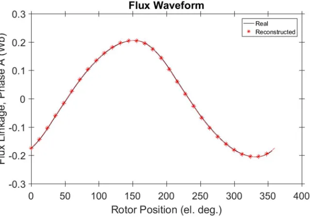
4.2.2 Flux-Linkage, Back EMF, and Torque Derivation
The radial flux per unit axial length Φ for one turn of a coil placed around a stator tooth seen in Fig. 4.6 is determined from the average magnetic vector potential in both coil sides as in (4.3) [30].
Φa a+ - =Aa+-Aa- (4.3)
Multiplication with the number of series turns per phase derives the flux linkage per unit of axial length of the machine. Applying the axial length of the machine then generates the flux linkage waveform of the motor seen in Fig. 4.7. All three phases can be reconstructed by applying a 120-degree phase shift to the waveform. A fast Fourier transformation (FFT) is performed to obtain the fundamental and harmonic content in the waveform. The waveform can therefore be modelled as a Fourier series of the
fundamental and harmonic components as seen in (4.4) where v is the harmonic order, λ
is the flux linkage, and ϕv is the phase angle for the vth harmonic. The maximum
harmonic order is a function of the number of magnetostatic solutions, s, as in (4.5).
Using five solutions produces 30 useable samples, which provides results that account for
harmonics up to the 14th order [30].
( )
(
)
1 cos
M v
a v v
v
v =
l q =
å
l q + f (4.4)3 1
M
v = s- (4.5)
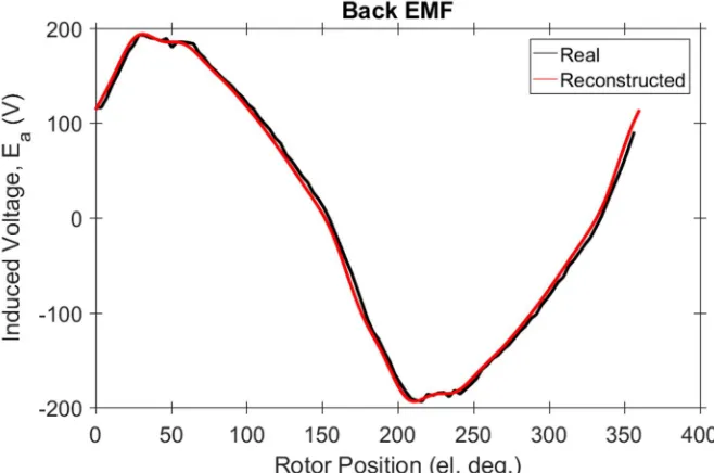
The back EMF ea waveform is obtained using (4.6) and is displayed in Fig. 4.8.
Similarly, the electromagnetic torque Tem is derived using (4.7) where i is the current and
P is the number of poles in the machine [38]. The electromagnetic torque waveform
37 Fig. 4.7. Flux-linkage waveform derived from FEA.
design to ensure that the motor will satisfy all driving conditions in a specific vehicle application. In an optimization scheme, the machine geometry gets manipulated and performance characteristics such as the average torque capability vary. Therefore, it is essential to develop a technique to maintain the capability of delivering the desired amount of torque for each motor model being generated by the optimization program [22].
( )
(
)
1 sin M v aa v v
v
d d
e v v
d dt =
l q
q = - =w l q + f
q
å
(4.6)( )
(
)
( )
(
)
( )
(
)
1 1
1
sin sin 120
2
sin 240
M M
M
v v
a v v b v v
v v
em v
c v v
v
i v v i v v P
T
i v v
= =
=
æ ö
ç q l q + f + q l q + f - ° +÷
ç ÷
= ç ÷
ç ÷
q l q + f - °
38 Fig. 4.8. Back EMF waveform derived from FEA.
Fig. 4.9. Continuous torque waveform derived from FEA.