Speeding up Reliability Analysis for Large-scale Circuits

University of Windsor University of Windsor

Scholarship at UWindsor

Scholarship at UWindsor

Electronic Theses and Dissertations Theses, Dissertations, and Major Papers

2016

Speeding up Reliability Analysis for Large-scale Circuits

Speeding up Reliability Analysis for Large-scale Circuits

Jinchen Cai

University of Windsor

Follow this and additional works at: https://scholar.uwindsor.ca/etd

Recommended Citation Recommended Citation

Cai, Jinchen, "Speeding up Reliability Analysis for Large-scale Circuits" (2016). Electronic Theses and Dissertations. 5804.

https://scholar.uwindsor.ca/etd/5804

This online database contains the full-text of PhD dissertations and Masters’ theses of University of Windsor students from 1954 forward. These documents are made available for personal study and research purposes only, in accordance with the Canadian Copyright Act and the Creative Commons license—CC BY-NC-ND (Attribution, Non-Commercial, No Derivative Works). Under this license, works must always be attributed to the copyright holder (original author), cannot be used for any commercial purposes, and may not be altered. Any other use would require the permission of the copyright holder. Students may inquire about withdrawing their dissertation and/or thesis from this database. For additional inquiries, please contact the repository administrator via email

Speeding up Reliability Analysis for Large-scale Circuits

By

Jinchen Cai

A Thesis

Submitted to the Faculty of Graduate Studies through Electrical and Computer Engineering in Partial Fulfillment of the Requirements for

the Degree of Master of Applied Science at the University of Windsor

Windsor, Ontario, Canada

2016

Speeding up Reliability Analysis for Large-scale Circuits

By

Jinchen Cai

APPROVED BY:

______________________________________________ Dr. Nader Zamani

Department of Mechanical, Automotive & Materials Engineering

______________________________________________ Dr. Rashid Rashidzadeh

Department of Electrical and Computer Engineering

______________________________________________ Dr. Chunhong Chen, Advisor

Department of Electrical and Computer Engineering

DECLARATION OF ORIGINALITY

I hereby certify that I am the sole author of this thesis and that no part of this thesis

has been published or submitted for publication.

I certify that, to the best of my knowledge, my thesis does not infringe upon anyone’s

copyright nor violate any proprietary rights and that any ideas, techniques, quotations, or

any other material from the work of other people included in my thesis, published or

otherwise, are fully acknowledged in accordance with the standard referencing practices.

Furthermore, to the extent that I have included copyrighted material that surpasses the

bounds of fair dealing within the meaning of the Canada Copyright Act, I certify that I have

obtained a written permission from the copyright owner(s) to include such material(s) in

my thesis and have included copies of such copyright clearances to my appendix.

I declare that this is a true copy of my thesis, including any final revisions, as approved

by my thesis committee and the Graduate Studies office, and that this thesis has not been

ABSTRACT

Reliability of logic circuits is becoming one of important concerns in the modern

integrated circuit design. A large number of inputs and signal correlations make reliability

analysis of logic circuits computationally expensive. Many reliabilities analysis

approaches have been proposed. Monte-Carlo simulation usually requires hours to obtain

a high precision result. Probabilistic gate models (PGM) just work perfectly for small

circuits or correlation-free circuits. Probability transfer matrices (PTM) and Bayesian

network techniques can give the accurate evaluations, but may become very

time-consuming and intractable for larger circuits. This thesis presents three new methods of

reliability analysis for large-scale circuits: (1) The improved equivalent reliability model

(2) Three-point method (3) The improved Monte Carlo simulation. They can increase the

evaluation efficiency and accuracy compared to the other existing approaches. These

ACKNOWLEDGEMENTS

Firstly, I appreciate my supervisor, Dr. Chunhong Chen, for his encouragement and

wise suggestions to my study and life. I have learned many things since I became Dr.

Chunhong Chen’s student. He spends very much time instructing me how to do research

and how to write papers.

I would like to thank Dr. Nader Zamani, the Outside Department Reader, for his

valuable time on reading and reviewing this thesis and coming up with valuable

suggestions.

I would like to appreciate Dr. Rashid Rashidzadeh, the Department Reader, for his

time and effort on reviewing this thesis with constructive comments.

Also, I wish to acknowledge the Department of Electrical and Computer Engineering.

Most of my theoretical foundations are built in here.,

Next, I am grateful to the help of Ran Xiao. Without his previous work on reliability

analysis, this master thesis would not be completed successfully.

Finally, I would like to show my deepest gratitude to my parents, Zhiyong Cai and

Min Zhang, for giving me a chance to study at the University of Windsor, financially

TABLE OF CONTENTS

DECLARATION OF ORIGINALITY ... III

ABSTRACT ... IV

ACKNOWLEDGEMENTS ... V

LIST OF TABLES ... VIII

LIST OF FIGURES ... IX

LIST OF ABBREVIATIONS ... X

CHAPTER 1 ... 1

INTRODUCTION ... 1

1.1 Motivations ... 1

1.2 Background and Prior Works ... 2

1.3 Organization of this thesis ... 3

CHAPTER 2 ... 5

THE IMPROVED EQUIVALENT RELIABILITY MODEL ... 5

2.1Previous Works ... 5

2.2ER Model ... 6

2.3 Improved ER Model ...11

2.4Simulation Results ... 14

CHAPTER 3 ... 17

THREE-POINT METHOD... 17

3.1 Previous Works ... 17

3.2 Three-point Method ... 18

3.3 Modified Model for Reliability Estimation ... 22

3.3.1 Q is close to A ... 22

3.3.2 Q is close to B ... 23

3.4 Simulation Results ... 25

THE IMPROVED MONTE CARLO SIMULATION ... 28

4.1Monte Carlo Simulation ... 28

4.2 Improved Monte Carlo Simulation ... 32

4.3Simulation Results ... 34

CHAPTER 5 ... 41

CONCLUSION AND FUTURE WORK ... 41

5.1 Conclusion ... 41

5.2 Future Work ... 42

REFERENCES ... 43

APPENDIX ... 46

LIST OF TABLES

Table I Output reliability vector R for different gates ... 9

Table II Computation of equivalent reliability pair at output for 2-input gates ... 10

Table III Computation of improved ER model and original ER model for performance

oniscas85 benchmark with 𝑟𝑔𝑎𝑡𝑒= 0.9 ... 15

Table IV Computation of improved ER model and original ER model for performance

oniscas85 benchmark with 𝑟𝑔𝑎𝑡𝑒= 0.95 ... 15

Table V Performance of the unmodified three-point Model on ISCAS’85 Benchmark

Circuits with 𝑟𝑔𝑎𝑡𝑒= 0.9 ... 21

Table VI Comparison of modified three-point model, three-point model and PGM on

ISCAS’85 Benchmark Circuits with 𝑟𝑔𝑎𝑡𝑒= 0.9 𝑃𝑖𝑛 = 0.5 ... 25

Table VII Comparison runtime of MTP and PGM on ISCAS’85 Benchmark Circuits

with 𝑟𝑔𝑎𝑡𝑒= 0.9 𝑃𝑖𝑛 = 0.5 ... 27

Table VIII 10 sets of random primary inputs with 𝑃𝑖𝑛 = 0.5 ... 31

Table IX 10 sets of error-free and measured value of primary output 1 and 2 ... 31

Table X Comparing the standard deviation when setting M=5000,1000,500,100, N

always be 1 of C499 circuit with 𝑟𝑔𝑎𝑡𝑒= 0.9 𝑃𝑖𝑛 = 0.5 ... 36

Table XI Comparing the error rate when setting M=5000,1000,500,100, N always be

LIST OF FIGURES

Fig 2 1 Equivalent reliability structure of a 2-input gate ... 6

Fig 2 2 Schematic of benchmark circuit C17... 12

Fig 2 3 The joint reliability 𝑟𝑎𝑏 of signals 6 and 8 in C17 ... 13

Fig 2 4 The joint reliability 𝑟𝑎𝑏 of signals 8 and 9 in C17 ... 13

Fig 3 1 The slope of tangent which passes through Q ... 19

Fig 3 2 Modified model for the case of PQ* ≥ α ... 23

Fig 3 3 Modified model for the case of PQ* ≤ β ... 24

Fig 4 1 Schematic of benchmark circuit C17... 30

LIST OF ABBREVIATIONS

CMOS – Complementary Metal Oxide Semiconductor

MCs – Monte-Carlo simulations

PGM – Probabilistic Gate Models

PTM – Probability Transfer Matrices

BDEC – Boolean Difference-based Error Calculator

ER – Equivalent Reliability

CHAPTER 1

INTRODUCTION

1.1 Motivations

As CMOS technology has been relied on shrinking dimension of the electrical device

for years, it has entered the nanometre regime. However, nanometer-scale electronic

components have less reliability than previous COMS devices due to their lower operating

temperature and higher sensitivity to random noises. At the same time, it puts forward

higher requirement in CMOS fabrication process. For instance, manufacturing imprecision

and interferences of impurities will degrade circuit reliability behavior. Therefore,

reliability issues have become challenges in current circuits and system design. So it draws

people’s great interest in reliability analysis.

Due to the exponentially growing number of circuit components and their complex

signal correlations, the complexity of reliability analysis for integrated circuit can be

prohibitively high. In order to address this issue, many approaches of reliability analysis

have been proposed. As a typical statistical method, Monte-Carlo simulation (MCs) has

been widely used for reliability evaluation [4]. Although accurate, the MCs would be very

time-consuming for the large circuit. Many analytical methods have also been proposed,

such as probabilistic gate models (PGM) [1], probability transfer matrices (PTM) [2],

Boolean difference-based error calculator (BDEC) [3] and so on. Although these

1.2 Background and Prior Works

Reliability of a logic signal is the probability that its value is correct [5]. Because of

possible errors with its driving gate, the signal may become unreliable. In 1956, Von

Neumann proposed there will be the same independent probability of error ε, that gate

output will appear a bit flip (from 0 to 1 or from 1 to 0) with by a binary symmetric channel

[6]. The error probability ε should belong to the range between 0 and 0.5. When ε equals

to 0, it means the gate is error-free. ε = 0.5 means the gate behavior is totally random. Since

the probability of failure should not be more than the probability of correctness in logic

circuit design, its value should not larger than 0.5. This assumption works well for the most

conventional circuits [5].

If gates in a circuit are assumed to error-free and only the primary inputs cause the

error, using simple algorithms can solve the problem of the reliability analysis. However,

the gates failure cannot be ignored in the real circuit. When considering the gate failure, the

reliability analysis seems more complicated because of the exponential number of

combinations. At the same time gates in the circuit are usually multiple inputs gates rather

than single input gates, so it is not independent between each gate. These factors cause

reliability analysis extremely complex [7].

Monte-Carlo simulation is a statistical approach to solve the problem of reliability

analysis. Reliability evaluation can also be achieved through some analytical approaches

Bayesian network [8]. The PGM method can provide accurate evaluation results for small

circuits with some certain probabilities of primary input but it may not work well for

correlation circuits. The PTM can also give the accurate evaluations but the runtime will

increase exponentially with the number of reconvergent fanouts. Furthermore, the

probability of occurrence of every input-output vector pair should be stored, which needs

a tremendous data storage. These problems also exist in Bayesian network approach and

more intractable to be solved. Alternatively, many hybrid analysis approaches have been

proposed. However, they may lose much in accuracy even on small circuits [5].

1.3 Organization of this thesis

This thesis is organized as follows.

Chapter 2 proposes the improved equivalent reliability model, introduces some

concepts of reliability and probability for reliability analysis, and explains the original ER

model and its drawback. Simulation results are provided to show the accuracy improvement

with improved method.

Chapter 3 presents a new approach which is named three-point method and explains

how to derive it. We will compare simulation results on benchmark circuits with existing

methods to provide the advantages of the proposed method in terms of either efficiency or

accuracy.

improved model which can estimate a simulation running times according to the setting of

error. Simulation results are shown to verify the validity of predicted times.

Chapter 5 concludes the thesis along with some future research works. The appendix

CHAPTER 2

THE IMPROVED EQUIVALENT RELIABILITY MODEL

In this section, the proposed method is improved equivalent reliability model, which

is also based on the concept of equivalent reliability. We improve the algorithm of the joint

reliability 𝑟𝑎𝑏 and the signal correlation coefficient in order to determine the reliability of

a circuit more accurately. But the main idea is not changed, which is still using the reliability

and probability information of inputs signal and gate information to estimate the equivalent

reliability of outputs. Equivalent reliabilities are propagated throughout the circuit base on

circuits’ topology. In this way, reliability of outputs actually shows the information of the

whole propagation path. So it ensures the accuracy of the method.

2.1Previous Works

We first introduce some concepts of reliability and probability. Normally, we use a

probability to represent the reliability, which does not distinguish two types of situations:

the signal of output equal to 0 or 1. So we proposed the concept of equivalent reliability.

Using the reliability pair instead of a single signal reliability. So any signal of a circuit is

associated with a reliability pair {req0, req1}, where req0 (or req1) represents the probability

of actual signal value and error-free signal value are both “0” (or “1”) over its error-free

value is “0” (or “1”). When the circuit is reliable, the output value is error-free, when the

correct. Specifically, for signal s, req0 = P {(s=s*)/(s*=0)} and req1= P {(s=s*)/(s*=1)},

where s* represents error-free version of s. The symbol “*” symbolizes “error-free”

(“reliable” or “correct”) in the thesis. 𝑃_𝑠(P{s=”1”}) is used to express the probability of

actual signal s (the probability of signal being logic “1”). So P{s=”0”} indicates the

probability of actual signal being logic “0”, which is equal to 1-𝑃𝑠. [1] 𝑃𝑠∗ (P{s*=”1”}

denotes the probability of signal s be logic “1” when the circuit is error-free, thus P{s*=”0”}

represents the probability of error-free signal s be logic “0” [5].

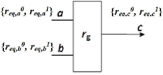
Consider a 2-input gate with reliability of 𝑟_𝑔, where {req,a0, req,a1} and {req,b0, req,b1}

denote the equivalent reliability pairs for input signals a and b respectively, where {req,c0,

req,c1} is the equivalent reliability pair for the output c,as shown in Fig. 2.1.

2.2ER Model

The problem of reliability analysis can be simply express as follow: using the

equivalent reliability pairs {req,a0, req,a1} and {req,b0, req,b1} of inputs and individual gate

reliability 𝑟_𝑔 to find the {req,c0, req,c1} and probability information 𝑝_𝐶∗ for output, the

average reliability of the output can be expressed by[5]

𝑟_𝑐 = 𝑝_𝑐∗_𝑟

𝑒𝑞,𝑐1 + (1 − 𝑝𝑐∗)𝑟𝑒𝑞,𝑐0 (2.1)

So the actual probability of the output can be represented as

𝑝_𝑐 = 𝑝_𝑐∗𝑟_{𝑒𝑞,𝑐}1 + (1 − 𝑝_𝑐∗)(1 − 𝑟_{𝑒𝑞,𝑐}0 _{) (2.2)}

The error-free input probability vector P* is defined as a 1×4 matrix where each

element represents a joint probability of error-free signals a* and b*, i.e., [5]

𝑃∗ _{= [𝑃}

00∗ 𝑃01∗ 𝑃10∗ 𝑃11∗ ]

= [P{𝑎∗_𝑏∗ _{= 00} P{𝑎}∗_𝑏∗ _{= 01} P{𝑎}∗_𝑏∗ _{= 10} P{𝑎}∗_𝑏∗ _{= 11}] (2.3)}

And the actual input probability P of actual signal a and b, i.e.,

𝑃 = [𝑃00 𝑃01 𝑃10 𝑃11]

= [P{𝑎𝑏 = 00} P{𝑎𝑏 = 01} P{𝑎𝑏 = 10} P{𝑎𝑏 = 11}] (2.4)

The relationship between 𝑃∗ and P can be written as [5]

𝑃 = 𝑃∗_{𝑀 (2.5)}

Where M is a 4×4 probability transfer matrix given by

               11 11 10 11 01 11 00 11 11 10 10 10 01 10 00 10 11 01 10 01 01 01 00 01 11 00 10 00 01 00 00 00 p p p p p p p p p p p p p p p p M (2.6)

where each element 𝑃_𝑖𝑗𝑘𝑗 represents a conditional probability for ab = kl given a*_b*₌

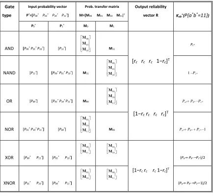
For a logic gate with two inputs signal a and b, the output reliability vector R is a 4×1

matrix where each element is a conditional probability for its output c being a specific value

k0 given ab = 00, 01, 10 or 11, i.e.,

R = [P{c = k0 | ab = 00} P{c = k0 | ab = 01} P{c = k0 | ab = 10} P{c = k0 | ab = 11}]T

where k0 = 0 for AND, NOR and XNOR gates, and k0 = 1 for NAND, OR and XOR gates.

Probability vector P* of Eq. (2.3) and vector M of Eq. (2.6) both can split into

sub-vector 𝑃₀∗ , 𝑃₁∗ and M₀ ,M₁ according to the combination of 𝑎∗ and 𝑏∗[5].

Let 𝐾_𝑎𝑏∗ {aa*_b* _{11}. The error-free input probability vector P}* _{of (2.3) can be}

rewritten as:

] 1

[ _{* *} * _* * _* * *

*

ab ab

a ab b

ab b

a P K P K P K K

P    

 

P _(2.7)

The vector 𝐾_𝑎𝑏∗ , R, 𝑃₀∗, 𝑃₁∗, M0 and M1 for different gates are different, which is

Table I Output reliability vector R for different gates

Gate

type

Input probability vector

P*_=[P

00* P01* P10* P11*]

Prob. transfer matrix

M=[M00 M01 M10 M11]T

Output reliability

vector R Kab*(P{a*b*=11})

P0* P1* M0 M1

AND [P00* P01* P10*] [P11*]           10 01 00 M M M M11

[rc rc rc 1−rc]T

Pc*

NAND [P11*] [P00* P01* P10*] M11           10 01 00 M M M

1 –Pc*

OR [P00*] [P01* P10* P11*] M00           11 10 01 M M M

[1−rc rc rc rc]T

Pa*+ Pb* –Pc*

NOR [P01* P10* P11*] [P00*]           11 10 01 M M M

M00 Pa*+ Pb* + Pc*–1

XOR [P00* P11*] [P01* P10*]

      11 00 M M       10 01 M M

[1−rc rc rc 1−rc]T

(Pa*+ Pb* –Pc*)/2

XNOR [P01* P10*] [P00* P11*]

      10 01 M M       11 00 M M

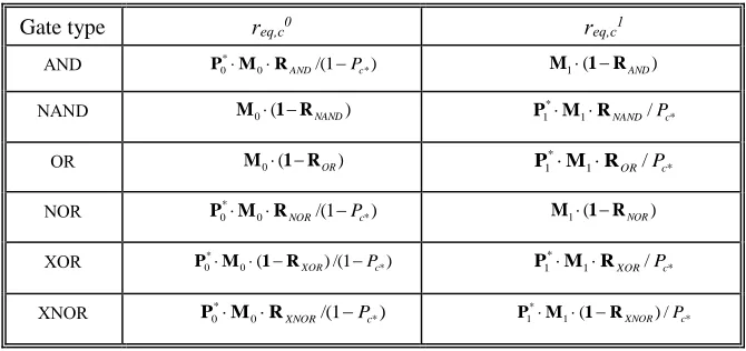
Table II shows the computation of equivalent reliability pair {req,c0, req,c1} for different

gates. Computation of equivalent reliability pair at output for 2-input gates

Table II Computation of equivalent reliability pair at output for 2-input gates

Gate type req,c0 req,c1

AND 0 /(1 *)

*

0M RAND Pc

P M₁(1R_AND)

NAND M0(1RNAND) 1 *

*

1 M RNAND/Pc

P  

OR M₀(1R_OR) * _{1 *}

1 M ROR/Pc

P  

NOR * ₀ /(1 _*)

0M RNOR Pc

P M1(1RNOR)

XOR 0 ( )/(1 *)

*

0M 1RXOR Pc

P * _{1 *}

1 M RXOR/Pc

P  

XNOR * ₀ /(1 _*)

0M RXNOR Pc

P 1 *

*

1 M (1 RXNOR)/Pc P   

Normally, the {req,a0, req,a1} and {req,b0, req,b1} of inputs are correlated, in order to reflect

the reliability correlation between them. We proposed a joint reliability as the conditional

probability which the actual input signals a and b are both correct.

So M of Eq. (2.6) becomes

                                 ab ab a ab b ab b a ab a ab ab b a ab b ab b ab b a ab ab a ab b a ab b ab a ab r r r r r r r r r r r r r r r r r r r r r r r r r r r r r r r r 1 1 1 1 ' M (2.8)

As we known, using Monte-Carlo simulation to estimate the joint reliability 𝑟_𝑎𝑏 is a

very time-consuming work for large circuits. Therefore, we proposed an efficient method

to estimate the 𝑟_𝑎𝑏 . The signal correlation coefficient between a*and b* of previous

1 0 , , )] ( 1 )[ ( )] ( 1 )[ ( ) ( ) ( } { θ * * * * * * * * previous j) (i, or j i j b P j b P i a P i a P j b P i a P ij b a P _             (2.9)

And the joint reliability 𝑟_𝑎𝑏(𝑖,𝑗)of previous method is:

(2.10)

It can be seen that the signal correlation coefficient between a* and b* and the joint

reliability 𝑟_𝑎𝑏(𝑖,𝑗) of original one is changed base on the different pairs (i, j). But we spotted

that the signal reliability correlation coefficient should use average value to meet all the

conditions, so Eq. (2.9) and (2.10) would lead to the large margin of error in some cases.

2.3 Improved ER Model

Thereby, we introduce the average sign correlation coefficient 𝑄∗ and the average

joint reliability 𝑟𝑎𝑏.In this case, the error bound of them will decrease. Improved method

requires 𝑟_𝑎 and 𝑟_𝑏 which value of reliability of inputs signal a and b, and the probability

of error-free signals a* and b*. The relationship between them as follows:

𝑃_𝑎𝑏∗ 𝑟_𝑎𝑏− 𝑃_𝑎∗_𝑟

𝑎𝑃𝑏∗𝑟𝑏= 𝑄∗• [2•min (𝑟𝑎, 𝑟𝑏)• 𝑟𝑔− 𝑟𝑔2+ max (𝑟𝑎, 𝑟𝑏) •{𝑟𝑔 − min (𝑟𝑎, 𝑟𝑏)}]

the signal correlation coefficient between a*and b* is

𝑄∗ _{= 𝑃}

𝑎𝑏∗ − 𝑃𝑎∗𝑃𝑏∗ (2.11)

So 𝑟_𝑎𝑏 as follows:

𝑟𝑎𝑏=

𝑄∗• [2•min (𝑟𝑎,𝑟𝑏)• 𝑟𝑔−𝑟𝑔2+max (𝑟𝑎,𝑟𝑏) •{𝑟𝑔−min (𝑟𝑎,𝑟𝑏)}]+𝑃𝑎∗𝑟𝑎𝑃𝑏∗𝑟𝑏

𝑃_𝑎𝑏∗ (2.12)

)

1

(

)

1

(

θ

ab

r

r

r

r

r

r

r

Where 𝑃_𝑎𝑏∗ is the maximum of (P {𝑎∗_𝑏∗ _{= 00}, P {𝑎}∗_𝑏∗ _{= 01}, P {𝑎}∗_𝑏∗ _{= 10}, P}

{𝑎∗_𝑏∗ _{= 11}),𝑃}

𝑎∗ 𝑎𝑛𝑑 𝑃𝑏∗ are corresponding values. For instance, if 𝑃01∗ is the maximum,

then let

𝑃_𝑎∗ = 𝑃₀∗ and 𝑃_𝑏∗ = 𝑃₁∗, so 𝑄∗=𝑃₀₁∗ _{− 𝑃}

0∗𝑃1∗.

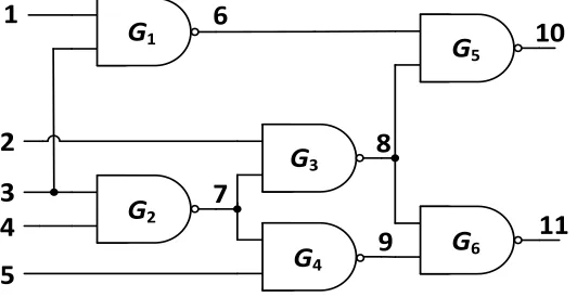
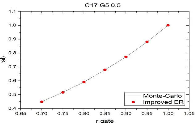
In order to verify the effects of Eq. (2.12), we took the circuit C17 as an example, as

shown in Fig. 2.2. Gate 5 has two correlated input signals 6 and 8. Gate 6 has two correlated

input signals 8 and 9. We compare the estimated values based on Eq. (2.12) with the

accurate 𝑟_𝑎𝑏 values which from Monte-Carlo simulation. Assuming primary input

probabilities is set to 0.5, and gate reliabilities 𝑟_𝑔 arrange from 0.7 to 1. The results of the

joint reliability of signal 6 and signal 8 is shown in Fig. 2.3, the joint reliability of signal 8

and signal 9 is shown in Fig. 2.4. It can be seen that the estimate results of the joint

reliability 𝑟_𝑎𝑏 are consistent with the accurate value.

1

2

3 4

5

G1

G2

G4

G3

G6

G5

6

7

8

9 11

10

Fig 2 3 The joint reliability 𝑟𝑎𝑏 of signals 6 and 8 in C17

The procedure of the improved equivalent reliability model can be summarized as

follows:

Input: Probability of primary inputs, gate reliabilities

Output: Reliability of primary outputs

Setp1: Sort gates base on circuits’ topology;

Calculate probabilities of all signal for error-free circuit;

Stpe2: For any gate as Fig. 2.1, obtain reliabilities 𝑟𝑎 and 𝑟𝑏 of inputs a and b

Find 𝐾_𝑎𝑏∗ , R, 𝑃₀∗_{, 𝑃}

1∗ from Table I;

Find M₀ and M₁ from Eq. (2.8) and Table I;

Calculate {req,c0, req,c1} of output c from Table II;

Step3: Calculate the overall reliability 𝑟_𝑐 of output c by Eq. (2.1);

Propagate it to the next gate.

2.4 Simulation Results

Simulations are all implemented in MATLAB with 2.40 GHz processor and 8GB

RAM. Setting the accurate reliability values are calculated by Monte-Carlo reliability

analysis.

We also took ISCAS85 benchmarks as an example to verify the performance and

computational efficiency of improved equivalent reliability model on large circuits in

probabilities is 0.5 with 𝑟_𝑔 =0.9 (Table III) and 0.95(Table IV). avg. error (%) max error (%) runtime:

T1 + T2 (s)

avg. error (%) max error (%) avg. error (%) max error (%) runtime:

T1 + T2 (s)

avg. error (%) max error (%) C17 6 5 2 0.48% 0.78% 0.906+0.017 0.10% 0.78% 1.17% 1.56% 0.906+0.017 0.22% 1.56% C432 160 36 7 3.59% 6.50% 29.494+0.036 1.05% 7.70% 8.46% 25.39% 29.494+0.035 1.63% 25.39% C499 202 41 32 2.94% 3.31% 35.805+0.038 1.36% 5.13% 0.20% 0.61% 35.805+0.036 0.24% 5.92% C880 383 60 26 1.88% 19.23% 55.644+0.049 1.54% 21.47% 3.33% 29.30% 55.644+0.047 2.75% 32.62% C1355 546 41 32 1.27% 1.57% 75.024+0.061 4.11% 22.70% 5.13% 5.53% 75.024+0.058 8.83% 49.39% C1908 880 33 25 4.39% 22.37% 132.049+0.075 4.15% 24.04% 6.28% 30.83% 132.049+0.071 5.30% 31.75% C2670 1193 233 140 1.61% 23.99% 194.606+0.100 1.97% 26.59% 3.21% 52.60% 194.606+0.094 4.57% 80.69% C3540 1669 50 22 11.20% 19.47% 295.022+0.140 2.29% 21.40% 13.91% 24.46% 295.022+0.124 5.46% 38.39% C5315 2307 178 123 2.73% 16.72% 599.330+0.2 2.50% 34.62% 6.23% 36.21% 599.330+0.205 4.92% 44.25% C7552 3512 207 108 5.26% 18.21% 2302.170+0.248 3.28% 34.51% 8.77% 26.77% 2302.170+0.232 5.81% 50.35%

3.54% 13.22% 2.23% 19.89% 5.67% 23.33% 3.97% 36.03%

Average

Circuit Size Inputs Outputs

Improved ER model Original ER model

OUTPUT All gate OUTPUT All gate

avg. error (%) max error (%) runtime:

T1 + T2 (s)

avg. error (%) max error (%) avg. error (%) max error (%) runtime:

T1 + T2 (s)

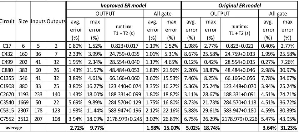
avg. error (%) max error (%) C17 6 5 2 0.80% 1.52% 0.823+0.017 0.19% 1.52% 1.98% 2.77% 0.823+0.021 0.40% 2.77% C432 160 36 7 2.33% 3.99% 24.759+0.035 1.01% 5.31% 8.67% 25.58% 24.759+0.033 1.99% 25.58% C499 202 41 32 1.95% 2.34% 28.554+0.040 1.17% 4.65% 0.12% 0.42% 28.554+0.035 0.27% 7.26% C880 383 60 26 1.43% 11.57% 48.484+0.053 1.83% 21.96% 2.20% 18.87% 48.484+0.046 2.98% 30.97% C1355 546 41 32 3.89% 4.61% 66.166+0.060 3.60% 15.53% 7.46% 8.25% 66.166+0.056 7.78% 34.67% C1908 880 33 25 3.80% 16.27% 123.440+0.074 3.35% 16.27% 5.36% 25.24% 123.448+0.070 3.94% 25.24% C2670 1193 233 140 1.43% 18.00% 188.331+0.099 1.80% 18.87% 3.11% 28.67% 188.331+0.091 4.51% 74.71% C3540 1669 50 22 5.69% 9.89% 284.570+0.129 1.75% 16.80% 8.73% 21.73% 284.570+0.118 4.51% 36.72% C5315 2307 178 123 1.93% 11.44% 583.947+0.196 2.12% 22.16% 5.88% 29.61% 583.947+0.180 4.59% 30.39% C7552 3512 207 108 3.94% 18.09% 2178.979+0.245 3.02% 26.89% 6.75% 26.29% 2178.979+0.226 5.47% 43.95%

2.72% 9.77% 1.98% 15.00% 5.02% 18.74% 3.64% 31.23%

average

Circuit Size Inputs Outputs

Improved ER model Original ER model

OUTPUT All gate OUTPUT All gate

Table III Computation of improved ER model and original ER model for performance oniscas85 benchmark with 𝑟𝑔𝑎𝑡𝑒= 0.9

It should be mentioned that the above error estimations of all methods in this thesis

are based on calculation of the absolute error, rather than calculating the relative error.

When calculating the relative error, errors will be offset by the positive and negative value,

thereby its value looks smaller than the absolute error. But it cannot really reflect the

performance of methods. So we used the absolute error to show the error.

It can be seen from both tables that the average error of improved ER model is around

3%, compared to the approximately 5% for the previous ER model, which decrease 2%

error of reliability. And the average value of maximum error drops significantly at the same

time. So the improved ER method can keep a better accuracy of reliability analysis than

the original one. The runtimes of two methods are barely changed, as shown in both tables,

which includes T1 that spent on calculating probabilities of all signals for error-free circuit

and T2 that spent on reliability analysis. Calculating probabilities of all signals is

time-consuming, but it is required only once with gate reliability change. Any change in the

circuit just requires an extra linear time for reliability analysis. So improved ER method

CHAPTER 3

THREE-POINT METHOD

In this section, the three-point method is presented for evaluating the reliability of

integrated circuit. Using the probability information (𝑃_𝐹 ,𝑃_𝐹∗ _{) for three points of same}

output with different 𝑃∗ and building a curve of their relationship. By evaluating

equivalent reliabilities through the information of curves, reliability analysis can be done

efficiently, while keeping a high level of accuracy.

3.1 Previous Works

In order to better analyze reliability, we also use the equivalent reliability of signal as

ER method. So any signal of a circuit is associated with a reliability pair {L, K}, as well as

reliability pair {req0, req1} of ER method. So for signal s, 𝐿 =P {(s=s*)/(s*=0)} and 𝐾= P

{(s=s*)/(s*=1)}. As above ER model, using three-point method to analyze circuit reliability,

we still need to know the probabilities of primary inputs and each gate reliabilities of circuit

at first. If the reliabilities pair {L, K} for the output could be found, the average reliability

for this output can be calculated as [5]

𝑟 = 𝑃∗𝐾 + (1 − 𝑃∗)𝐿 (3.1)

At the same time, the single signal reliability can be defined as another reliability pair

{𝑟0_{, 𝑟}1_{}. 𝑟}0 _{(or 𝑟}1_{) is defined as the probability that the actual signal and error-free signal}

reliability pair for the output signal F is derived as

𝑟_𝐹0 = (1 − 𝑝_𝐹∗_)𝐿

𝐹

𝑟_𝐹1 = 𝑃_𝐹∗𝐾_𝐹 (3.2)

Therefore, we need to find the reliabilities pair {L, K} at first. As probabilities of

primary inputs and each gate reliabilities of the circuit are given. P and P* can be calculated

by Monte-Carlo simulation or PGM, which P is the probability of actual output signal F

(when the circuit is unreliable), whereas P* is the probability of error-free output signal F

when the circuit is reliable [9]. So the equation between 𝑃_𝐹∗ _{and 𝑃}

𝐹 can be expressed as

𝑃𝐹 = 𝑟𝐹1+1 − 𝑃𝐹∗−𝑟𝐹0

= 𝑃_𝐹∗_𝐾

𝐹+ 1 − 𝑃𝐹∗− (1 − 𝑃𝐹∗)𝐿𝐹 (3.3)

3.2 Three-point Method

In what follows, we show how to the reliability pair {L, K}, first we assume the 𝐾_𝐹

and 𝐿_𝐹 is linear equation of 𝑃_𝐹∗, so

𝐾_𝐹 = 𝛼₁𝑃_𝐹∗+𝛽₁

𝐿𝐹 = 𝛼2𝑃𝐹∗+𝛽2 (3.4)

Where 𝛼1, 𝛼2, 𝛽1, 𝛽2 are all constant, then we put Eq. (4) into Eq. (3) becomes

𝑃_𝐹 = (𝛼₁+ 𝛼₂)𝑃_𝐹∗2+(𝛽₁+ 𝛽₂− 1 − 𝛼₂)𝑃_𝐹∗− 𝛽₂+ 1

It can be seen that 𝑃_𝐹 is quadratic equation of 𝑃_𝐹∗_{, it can be rewritten as}

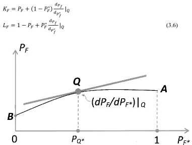
We can see that 𝑃_𝐹 is a quadratic curve, as shown in Fig. 3.1. (setting 𝑃_𝐹∗ as X axis

and 𝑃_𝐹 as Y axis) Therefore, we need at least 3 points to determine it. They are check point,

𝑃_𝐹∗ = 0 point and 𝑃_𝐹∗ = 1 point respectively. In order to analyze conveniently, check point

is defined as Q, 𝑃_𝐹∗ _{= 0 𝑎𝑛𝑑 𝑃}

𝐹∗ = 1 are defined as B, A respectively. As shown in Fig.

3.1, the slope of tangent which passes through Q is 𝑑𝑃𝐹

𝑑

𝑃𝐹∗

|_𝑄, and it is equal to the ratio of

𝑃𝐹 variation to 𝑃𝐹∗ variation ( ∆𝑃𝐹

∆𝑃𝐹∗). Therefore, the reliabilities pair {𝐿𝐹, 𝐾𝐹} of signal F can

be expressed by 𝑃𝐹 and 𝑃𝐹∗

𝐾_𝐹 = 𝑃_𝐹+ (1 − 𝑃_𝐹∗) 𝑑𝑃𝑓

𝑑_𝑃𝑓∗ |𝑄

𝐿_𝐹 = 1 − 𝑃_𝐹+ 𝑃_𝐹∗ 𝑑𝑃𝑓

𝑑_𝑃𝑓∗ |𝑄 (3.6)

Fig 3 1 The slope of tangent which passes through Q

When the probability of primary inputs and gate reliabilities are set, 𝑃𝐹 and 𝑃𝐹∗ of

outputs could be achieved by the method of PGM. In order to get more accurate value, we

Pf* cannot always be 0 or 1[10]. For seeking out 𝑃_𝐹∗_{=0 and 𝑃}

𝐹∗=1 points, we set signals of

inputs as permanent signals rather than a probability. In this way, the point which PF* is

equal to 0 or 1 will be found. Then we change the input signal with other permanent signals,

until we find A and B two points of each outputs. When 𝑃_𝐹 𝑎𝑛𝑑 𝑃_𝐹∗ of A, B, Q are found,

building a ternary linear equation, factors a, b and c can be figured out from Eq. (5). 𝑑𝑃𝐹

𝑑

𝑃𝐹∗

|_𝑄

is obtained by taking the derivative of this Eq. (3.5) as follows:

𝑑_𝑃𝐹 𝑑

𝑃𝐹∗

|_𝑄 = 2𝑎𝑃_𝐹∗+ 𝑏 (3.7)

By using Eq. (3.7), Eq. (3.6) can be rewritten as

𝐾_𝐹 = 𝑃_𝐹− 2a𝑃_𝐹∗2+ (2a − b)𝑃_𝐹∗+ 𝑏

𝐿𝐹 = 1 − 𝑃𝐹+ 2a𝑃𝐹∗2+ 𝑏𝑃𝐹∗ (3.8)

We obtain the value of reliabilities pair {L, K} of each output from Eq. (3.8) and put

it into Eq. (3.1). Finally, the reliability of each gate Eq. (3.1) becomes

𝑟_𝐹 = 2𝑃_𝐹𝑃_𝐹∗2_{− 4𝑎𝑃}

𝐹∗3+ (4𝑎 − 2𝑏)𝑃𝐹∗2+ (2𝑏 − 1)𝑃𝐹∗+ 1 − 𝑃𝐹 (3.9)

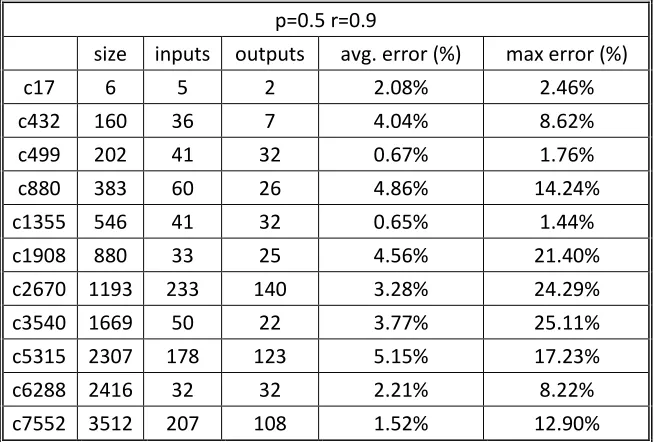
We took ISCAS85 benchmarks to test the performance of the three-point method on

large circuits. The proposed three-point was implemented in MATLAB. The value of

Monte-Carlo reliability estimation is accurate value. Assuming the primary input

probability is 0.5 and all gate reliability is 0.9, simulation results are shown in Table V. The

average error and maximum error are both got from all primary outputs of circuits. Here,

the average (or maximum) error is defined as an average (or maximum) of (|𝑟_{𝐹.𝑒𝑠𝑡}− 𝑟_{𝐹.𝑎𝑐𝑐}|

accurate reliability values. It can be seen that the average error of it is around 1-4% in most

cases. For the worst case, maximum error would up to 25%.

Table V Performance of the unmodified three-point Model on ISCAS’85 Benchmark Circuits with 𝑟𝑔𝑎𝑡𝑒= 0.9

p=0.5 r=0.9

size inputs outputs avg. error (%) max error (%)

c17 6 5 2 2.08% 2.46%

c432 160 36 7 4.04% 8.62%

c499 202 41 32 0.67% 1.76%

c880 383 60 26 4.86% 14.24%

c1355 546 41 32 0.65% 1.44%

c1908 880 33 25 4.56% 21.40%

c2670 1193 233 140 3.28% 24.29%

c3540 1669 50 22 3.77% 25.11%

c5315 2307 178 123 5.15% 17.23%

c6288 2416 32 32 2.21% 8.22%

c7552 3512 207 108 1.52% 12.90%

After analyzing, these worst case always happen when 𝑃_𝐹∗ close to 0 or 1 in specific

circuits. Due to the variations of 𝑃_𝐴 and 𝑃_𝐵,it will cause the tangent passes through point

Q which closes to B and A extremely unstable and the slope will change in a large rang,

thereby rising errors in estimating reliability. Strictly speaking, if 𝑃𝐴 and 𝑃𝐵 could be

chosen as an average of the output probabilities over all inputs vectors which lead to PF*

= 1 and PF* = 0, it can completely eliminate this problem. But it is very high

time-consuming. In the following, we deal with these issues by modifying previous reliability

3.3 Modified Model for Reliability Estimation

In order to reduce the impact of variations of 𝑃_𝐴 and 𝑃_𝐵 on the reliability estimation

(when the point Q locates near to B or A), we take a straight line from Q to B (or A) instead

of using Eq. (3.5) to estimate 𝑑𝑃𝐹

𝑑_𝑃𝐹∗ |𝑄(the slope of tangent which passes through Q). The

following two cases will be discussed in details.

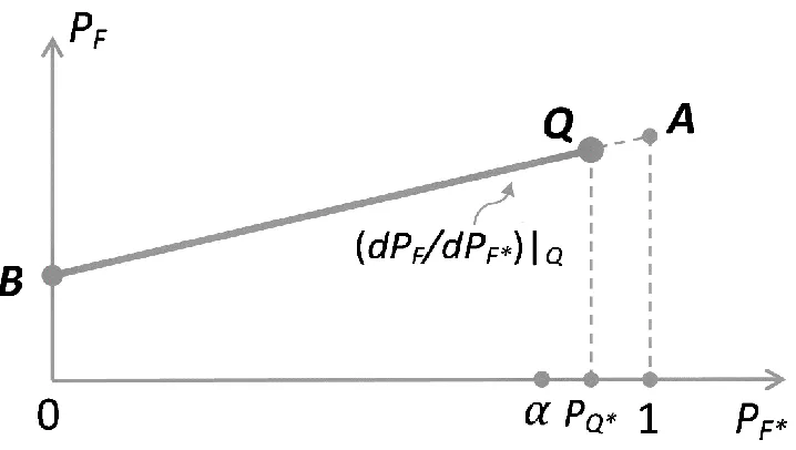
3.3.1 Q is close to A

If Q is close to A, then a straight line which through B and Q will be used to estimate

𝑑_𝑃𝐹

𝑑_𝑃𝐹∗ |𝑄. In order to define what situation is Q close to A, value α which is a threshold value

close to 1 is proposed. So 𝑃_𝑄∗ ≥ α is meaning Q locates close to A, as shown in Fig. 3.2. By

using a=0, the Eq. (3.5) translates to 𝑃_𝐹 = 𝑏𝑃_𝐹∗+ 𝑐, so 𝑏 = 𝑑𝑃𝐹

𝑑

𝑃𝐹∗

|_𝑄 =(𝑃_𝑄 ─ 𝑃_𝐵)/ 𝑃_𝑄∗ _and

c = 𝑃𝐵.This along with Eq. (3.6) can be rewritten as

𝐾 ≈ (𝑃𝑄+ 𝑃𝐵𝑃𝑄∗− 𝑃𝐵)/𝑃𝑄∗

𝐿 ≈ 1 − 𝑃𝐵

According to Eq. (3.1), it becomes

𝑟_𝐹 ≈ 𝑃_𝑄+ (1 − 𝑃_𝑄∗)(1 − 2𝑃_𝐵) (3.10)

𝑃_𝐵 may be unavailable in sometimes, especially when 𝑃_𝑄∗ is very close to 1. We

assume 𝑃_𝐵 ≈ 1 − 𝑟_𝐹.Thus , Eq. (3.10) can be modified as

Fig 3 2 Modified model for the case of PQ* ≥ α

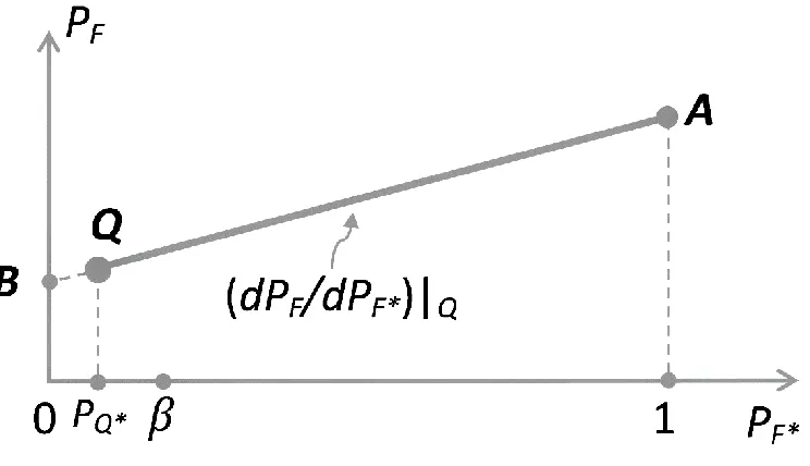
3.3.2 Q is close to B

If Q is close to B, then a straight line which through Q and A will be used to find

𝑑_𝑃𝐹

𝑑_𝑃𝐹∗ |𝑄. As same as the threshold value α, value β is a threshold value close to 0. So 𝑃𝑄

∗ _≤

β and Q locates close to B have the same meaning, as shown in Fig. 3.3. By using a=0, the

Eq. (3.5) becomes 𝑃_𝐹 = 𝑏𝑃_𝐹∗+ 𝑐 again, but 𝑏 = 𝑑𝑃𝐹

𝑑_𝑃𝐹∗ |𝑄=(𝑃𝐴 ─ 𝑃𝑄)/ (1 − 𝑃𝑄

∗_{) and c =}

(𝑃_𝑄 ─𝑃_𝐴𝑃_𝑄∗ )/ (1 − 𝑃_𝑄∗). This along with Eq. (6) can be rewritten as

𝐾 ≈ 𝑃_𝐴

𝐿 ≈ (1 − 𝑃_𝑄+ 𝑃_𝐴𝑃_𝑄∗− 𝑃_𝑄∗)/ (1 − 𝑃_𝑄∗)

According to Eq. (3.1), it becomes

𝑟_𝐹 ≈ 1 − 𝑃_𝑄− 𝑃_𝑄∗(1 − 2𝑃_𝐴) (3.12)

𝑃_𝐴 may be unavailable in sometimes, especially when 𝑃_𝑄∗ is very close to 0. At this

point, we assume 𝑃𝐴 ≈ 𝑟𝐹.Thus , Eq. (3.10) can be modified as

Fig 3 3 Modified model for the case of PQ* ≤ β

It can be seen that Eq. (3.11) and Eq. (3.13) are exactly same. So when Q is very close

to B (or A), 𝑟_𝐹 is used the Eq. (11) or Eq. (13) to estimate. The 𝑟_𝐹 variation of Eq. (3.12)

and Eq. (3.14) is given approximately by ∆𝑟_𝐹= 2𝛿_𝑚(1 − 𝑃_𝑄∗)𝑃_𝑄∗ . where 2𝛿_𝑚 is 𝑟_𝐹

variation under the worst case. Thus, when 𝑃_𝑄∗ is close 1 or 0, 𝑟_𝐹 variation is minimum.

For example, if 𝑃_𝑄∗ equal to 0.9, 𝑟_𝐹 variation is 9% of 2δm.

In summary, when Q locates in between (β< 𝑃_𝑄∗< α), we still use previous equation

(3.9) to estimate reliability 𝑟𝐹.When Q is close to B (𝑃𝑄∗ ≤β) or A (𝑃𝑄∗ ≥ α), Eq. (3.11) and

Eq. (3.13) are used to estimate output reliability 𝑟_𝐹 instead of Eq. (3.9). It should be

3.4 Simulation Results

After the change, we still took ISCAS85 benchmarks to verify the performance of the

modified three-point method on large circuits. It was also implemented in MATLAB with

𝑟_{𝑔𝑎𝑡𝑒} = 0.9 and 𝑃_𝑖𝑛 = 0.5. Simulation results are shown in Table VI. The average error

and maximum error are still got from all primary outputs of circuits and Error algorithm

does not change. After comparing with the previous three-point method, it can be seen that

the average error of modified three-point method drops obviously.

Table VI Comparison of modified three-point model, three-point model and PGM on ISCAS’85 Benchmark Circuits with 𝑟𝑔𝑎𝑡𝑒= 0.9 𝑃𝑖𝑛= 0.5

𝑟𝑔𝑎𝑡𝑒= 0.9 and 𝑃𝑖𝑛 = 0.5

circuit size inputs outputs avg. error (%)

modified unmodified PGM

c17 6 5 2 2.08% 2.08% 33.15%

c432 160 36 7 2.88% 4.04% 4.37%

c499 202 41 32 0.62% 0.67% 34.21%

c880 383 60 26 1.83% 4.86% 8.63%

c1355 546 41 32 0.65% 0.65% 21.53%

c1908 880 33 25 4.56% 4.56% 17.31%

c2670 1193 233 140 2.83% 3.28% 17.80%

c3540 1669 50 22 2.74% 3.77% 19.57%

c5315 2307 178 123 4.81% 5.15% 7.94%

c6288 2416 32 32 0.95% 2.21% 4.21%

c7552 3512 207 108 1.23% 1.52% 20.73%

In order to further demonstrate the efficiency of the modified three-point method(MTP)

on large circuits, we took ISCAS85 benchmarks as examples. It is well known that

Monte-Carlo is the most time-consuming method, so the runtime of it does not show in the table.

We only compare the runtime with PGM. We took 103 _{samples of input vectors for PGM}

simulation. The runtimes of MTP can be divided into two parts T1 and T2. T1 is the time

which spends on estimate 𝑃𝐹 𝑎𝑛𝑑 𝑃𝐹∗ of check point, 𝑃𝐹∗ = 0 point and 𝑃𝐹∗ = 1 point.

T2 is the time which is spent on using Eq. (3.13) to calculate the reliability of outputs. It

can be seen from the table VII, T2 is too small relative to T1 and just take linear time for

any large circuits. It is the key to improving efficiency, rather than exponential growth with

the growing number of gates for some other method. T1 is extremely big in runtime,

because we used Monte-Carlo method to simulate the 𝑃_𝐹 𝑎𝑛𝑑 𝑃_𝐹∗ of three points. 𝑃_𝐹∗=

0 point and 𝑃_𝐹∗ = 1 point of each output is not easy to be found in a small number of

simulation times. For reducing T1, there are many efficient approaches have been available

to find 𝑃𝐹 𝑎𝑛𝑑 𝑃𝐹∗ of three points instead of MC method. If using PGM, the total runtime

Table VII Comparison runtime of MTP and PGM on ISCAS’85 Benchmark Circuits with 𝑟𝑔𝑎𝑡𝑒= 0.9 𝑃𝑖𝑛= 0.5

𝑟𝑔𝑎𝑡𝑒= 0.9 and 𝑃𝑖𝑛 = 0.5

circuit size inputs outputs

Modified three-point

method PGM

Runtime(s): T1+T2 Runtime(s)

c17 6 5 2 0.366+0.01 0.030

c432 160 36 7 23.826+0.012 4.920

c499 202 41 32 38.208+0.01 4.970

c880 383 60 26 83.363+0.02 9.820

c1355 546 41 32 58.385+0.06 13.140

c1908 880 33 25 131.967+0.01 18.340

c2670 1193 233 140 515.582+0.016 27.020

c3540 1669 50 22 352.090+0.067 38.800

c5315 2307 178 123 1022.658+0.02 62.110

c6288 2416 32 32 423.271+0.012 50.340

CHAPTER 4

THE IMPROVED MONTE CARLO SIMULATION

Monte-Carlo simulation (MCs) is a computational algorithm which relies on random

sampling to obtain numerical results. It has been widely used for integrated circuit

reliability evaluation. However, it needs a common large number of analyses for any circuit,

which causing excessively time consuming. we presented a new method for calculating the

reliability of integrated circuit within the margin of setting error by improved Monte Carlo

simulation that can evaluate a simulation times according to different confidence levels and

different circuits, rather than previous MCs uses a large common simulations times for any

circuit. It can decrease unnecessary calculation time and increase the efficiency of

simulation dramatically.

4.1Monte Carlo Simulation

Monte Carlo technique is a sampling technique that is based on the probabilities to

solve stochastic problems. It also can be applied for sampling random variables from

probability distributions, so it has been widely used for reliability evaluation.

In the MCS, the binary bit streams are randomly generated by probabilities of the

signal. Bernoulli sequences are often used as binary bit streams in stochastic computation

[11, 12]. It independently generates a sequence of bits with the probability 𝑝 [13]. For

(20% to be logic “0”).

Consider a 2-input NAND gate. Which has two inputs a and b and one output c.

Assuming these two inputs are not correlated, the signal of input a and b random become

logic “0” or logic “1” base on 𝑃. If this gate is error-free, output signal C can be calculated

by the Boolean operation. Using C* to indicate the error-free version of sign C. If this gate

has a probability of error ε (the reliability of this gate is 1-ε), so the output c could be error

with probability ε. For example, if the input vector ab is “10”, when the gate is error-free,

the output signal c will be “1” (C*=1). When the gate is unreliable, the output signal C will

have probability ε to make it equal to “0”.

In Fig.4.1, a general stochastic model of NAND is used to illustrate this situation.

As a circuit, if probabilities of primary inputs and reliabilities of all the individual

gates are known, then the reliabilities of individual primary outputs could be calculated.

When this circuit has n inputs and m outputs, 𝐼₁, 𝐼₂… 𝐼_𝑛 stand for primary inputs and

𝑂1, 𝑂2… 𝑂𝑚 stand for primary outputs. N independent sets of values 𝐼1, 𝐼2… 𝐼𝑛 are

generated based on the probability of primary inputs. Assuming all gates in the circuit are

reliable, N sets of complete correct primary output 𝑂₁∗, 𝑂₂∗… 𝑂𝑚∗ can be calculated. There

N sets prime inputs 𝐼1, 𝐼2… 𝐼𝑛 are taken as input of measured circuit at the same time. Then

N sets of outputs signals 𝑂1, 𝑂2… 𝑂𝑚 of measured circuit will also be obtained. For output

o, comparing each set of error-free signal 𝑂_𝑜∗ _{with corresponding actual signal 𝑂}

𝑜, 𝑁𝑜 is

𝑃_𝑜 = 𝑁𝑜 𝑁

Fig 4 1 Schematic of benchmark circuit C17

So the reliability of this output o is 𝑟𝑜= 1 − 𝑃𝑜.

We took the C17 as an example, as shown in Fig. 1. The probability of primary inputs

𝑃 and reliability of gates r are assumed as 0.5 and 0.9 respectively. Table VIII is 10 sets of

signals of random primary inputs according to 𝑃. Table IX is 10 sets of signals of two

primary outputs for error-free circuit and measured circuit. The reliability of output can be

achieved from the Table IX. Taking Output2 as an example, there are 2 times that 𝑂_{𝑜𝑢𝑡𝑝𝑢𝑡2}∗

and 𝑂𝑜𝑢𝑡𝑝𝑢𝑡2 is not equal. So the failure probability of Output2 is 𝑃𝑜𝑢𝑡𝑝𝑢𝑡2= 2 10 ,

reliability of Output2 𝑟_{𝑜𝑢𝑡𝑝𝑢𝑡2} = 0.8. It is the general theory of Monte Carlo simulation.

Normally, MCS requires a large number of sets of random variables. So 10 sets of

random variables are completely sufficient. Therefore,𝑟_{𝑜𝑢𝑡𝑝𝑢𝑡2} = 0.8 is not strictly true.

pseudo-random numbers are required to cover as much as possible situations, which will

lead a large number of analysis running times needed to be operated for the stable outputs.

Therefore, the calculation time will increase exponential with the growing numbers of gates.

Table VIII 10 sets of random primary inputs with 𝑃𝑖𝑛= 0.5

Table IX 10 sets of error-free and measured value of primary output 1 and 2

Output Version 1 2 3 4 5 6 7 8 9 10

Output1 𝑂𝑜𝑢𝑡𝑝𝑢𝑡1

∗ _{1 0 0 0 1 1 1 1 1 1}

𝑂𝑜𝑢𝑡𝑝𝑢𝑡1 1 0 0 0 1 1 1 1 1 1

Output2 𝑂𝑜𝑢𝑡𝑝𝑢𝑡2

∗ _{1 0 0 1 0 1 0 1 0 1}

𝑂𝑜𝑢𝑡𝑝𝑢𝑡𝑠2 1 0 1 1 0 0 0 1 0 1

Set

Input 1 2 3 4 5 6 7 8 9 10

Input1 0 0 1 0 1 1 1 1 1 1

Input2 1 0 0 0 1 1 0 1 0 0

Input3 0 1 0 0 1 0 1 0 1 1

Input4 0 0 1 0 1 0 1 0 1 0

4.2 Improved Monte Carlo Simulation

In order to improve the efficiency of Monte Carlo simulation, we proposed the

improved Monte Carlo simulation. From the previous paper, there are still 1% - 5% error

when many existing analytical approaches could work well. While calculation precision of

previous Monte Carlo simulation cannot be controlled. One million simulation runs could

achieve 99.9% precision, but this number is so abstract for different size circuits. For C17

circuit which has five inputs, so there are total 25 different input combinations [14]. In this

case, one million simulation runs are too large. Many unnecessary computations consume

large time. While C7552 circuit has 207 inputs, so 2207 inputs combinations can cover all

the possibilities. Therefore, one million runs are too small for this circuit.

It is well known that the higher precision of reliability analysis is better, but higher

precision will consume more time. When the precision reaches one certain level, the

required running times that can increase 0.1% precision may need more than total previous

running times. In this paper, Improved Monte Carlo simulation is proposed. It could adjust

the number of simulation runs base on the size and complexity of the circuits when the

accuracy has been determined.

The convergence rate for each output of the same circuit is different, which can be

influenced even by the variance of the probability of primary inputs and individual gate

reliabilities [15]. Therefore, preliminary testing on convergence rate before the formal

the confidence interval of reliability 𝑟 could be estimated, is

(𝜇 − t ∙ 𝜎

√𝑁𝑠, 𝜇 + t ∙

𝜎

√𝑁𝑠) (4.1) [16]

Where t is the value based on a certain confidence level α.

Eq. (4.1) can be rewritten as

𝜇 − t ∙ 𝜎

√𝑁𝑠< 𝑟 < 𝜇 + t ∙

𝜎

√𝑁𝑠

Once the error tolerance ɛ is set, the total number of simulation 𝑁𝑠 can be calculated

as

{

|𝜇 − 𝑟| < t ∙ 𝜎

√𝑁𝑠

𝑟 < 𝜇 + t ∙ 𝜎

√𝑁𝑠

ɛ >|𝜇−𝑟|

𝑟

⇒ 𝜇∙ɛ

1−ɛ> t ∙ 𝜎 √𝑁𝑠

⇒ 𝑁_𝑠 > {t∙𝜎∙(1−ɛ)

𝜇∙ɛ } 2

(4.2)

Through the previous experiments, an empirical theory can be obtained. The

procedure can be summarized as follows:

Input: Probability of primary inputs, gate reliabilities and error tolerance

Output: Number of simulation

Step1: Randomly generate one set of input signal according to the probability of

primary inputs;

Step2: Put the above one set of input signal into the error-free circuit and the actual

Find out the reliability of outputs for running N times.;

Step3: Repeat step 1 and 2 M times. Each output will have M values of reliability；

(Note: This is different from previous Monte Carlo approach, which needs randomly

generate n sets of different inputs.)

Get the running times of the test is N*M;

Step4: Analyze the Gaussian distribution of M sets of reliability;

Calculate the standard deviation 𝜎 and mean μ of each output.

Step5: Obtain the value of t base on confidence level α from the probability table;

Compute the total simulation times 𝑁_𝑠 using Eq. (4.2).

4.3Simulation Results

The proposed IMCS approach was implemented in MATLAB. The result from

previous MCS runs one million is used as the standard result. Assuming N equals to 1000,

100, 10, 1 separately and increasing the value of M gradually. Through equation 1, 𝑁_𝑠 has

a linear relationship with variance (𝜎2_{). So the variance of standard deviation plays an}

important impact on 𝑁𝑠. According to the tests results, when N equals to 100, 𝜎 of some

outputs will change twice times with M increasing. When N equals to 1000, this

phenomenon will occur more obviously and the value of 𝜎 even have 7 times of change

with the increasing value of M. But when N=1, the value of the standard deviation σ hardly

We adopt C499 circuit of ISCAS85 benchmark as simulation object (assuming

primary input probabilities is 0.5 and all gates reliabilities are 0.9) and set 𝜎 which is

achieved from 104 text times (M=104 _{, N=1) as standard 𝜎(𝜎}

10000) .Using it compares

with other standard deviations when setting M=5000,1000,500,100, N always be 1. It can

be seen that from the table X, each ratio of standard deviation 𝜎 to 𝜎10000 is trend to 1,

which means when N=1, the standard deviation 𝜎 is nearly unchanged with M increasing.

M=10000 N=1

σ σ σ σ σ

724 0.433 0.430 0.995 0.421 0.973 0.429 0.991 0.469 1.084 0.443 1.024

725 0.430 0.426 0.992 0.419 0.975 0.421 0.980 0.394 0.917 0.418 0.973

726 0.431 0.421 0.977 0.426 0.988 0.411 0.952 0.441 1.022 0.404 0.937

727 0.427 0.422 0.988 0.424 0.993 0.420 0.983 0.446 1.045 0.443 1.037

728 0.430 0.430 0.999 0.433 1.006 0.426 0.991 0.423 0.983 0.485 1.127

729 0.425 0.434 1.021 0.433 1.021 0.436 1.026 0.409 0.964 0.404 0.952

730 0.428 0.425 0.992 0.434 1.015 0.428 0.999 0.461 1.076 0.463 1.082

731 0.425 0.421 0.990 0.431 1.013 0.417 0.982 0.402 0.945 0.471 1.108

732 0.423 0.436 1.031 0.424 1.002 0.419 0.991 0.409 0.969 0.443 1.048

733 0.429 0.426 0.994 0.424 0.988 0.423 0.986 0.465 1.084 0.388 0.905

734 0.427 0.430 1.007 0.422 0.987 0.420 0.983 0.441 1.032 0.443 1.037

735 0.427 0.426 1.000 0.429 1.006 0.417 0.978 0.409 0.960 0.404 0.947

736 0.430 0.421 0.979 0.427 0.992 0.420 0.976 0.423 0.983 0.443 1.030

737 0.429 0.431 1.005 0.435 1.014 0.433 1.011 0.402 0.937 0.418 0.976

738 0.425 0.423 0.995 0.426 1.002 0.416 0.978 0.429 1.009 0.443 1.042

739 0.430 0.428 0.996 0.430 1.002 0.446 1.039 0.435 1.013 0.418 0.974

740 0.425 0.420 0.989 0.437 1.030 0.437 1.029 0.429 1.011 0.454 1.068

741 0.430 0.427 0.993 0.419 0.974 0.412 0.957 0.394 0.916 0.404 0.939

742 0.430 0.434 1.010 0.436 1.013 0.394 0.917 0.409 0.952 0.485 1.128

743 0.426 0.430 1.011 0.416 0.977 0.399 0.937 0.409 0.962 0.388 0.912

744 0.428 0.426 0.995 0.419 0.980 0.425 0.993 0.456 1.066 0.404 0.944

745 0.430 0.430 0.998 0.433 1.007 0.406 0.944 0.465 1.080 0.454 1.054

746 0.429 0.430 1.003 0.434 1.012 0.436 1.016 0.441 1.028 0.418 0.976

747 0.429 0.431 1.003 0.429 0.999 0.430 1.001 0.429 1.000 0.431 1.005

748 0.430 0.429 0.999 0.429 0.998 0.439 1.022 0.423 0.985 0.328 0.764

749 0.428 0.430 1.005 0.422 0.985 0.432 1.010 0.429 1.003 0.471 1.101

750 0.427 0.432 1.011 0.419 0.981 0.430 1.007 0.416 0.975 0.463 1.084

751 0.425 0.430 1.012 0.422 0.993 0.412 0.970 0.394 0.928 0.418 0.985

752 0.427 0.425 0.993 0.436 1.020 0.444 1.040 0.402 0.940 0.463 1.083

753 0.426 0.432 1.013 0.438 1.027 0.448 1.053 0.465 1.091 0.431 1.013

754 0.429 0.422 0.985 0.437 1.020 0.435 1.014 0.409 0.955 0.485 1.131

755 0.429 0.426 0.994 0.429 1.001 0.447 1.044 0.409 0.955 0.454 1.058

output M=5000 N=1 M=1000 N=1 M=500 N=1 M=100 N=1 M=50 N=1

𝜎_{10000 𝜎/𝜎10000 𝜎/𝜎}

10000 𝜎/𝜎10000 𝜎/𝜎10000 𝜎/𝜎10000

Through the Eq. (4.2), 𝑁_𝑠 is inversely proportional to 𝜇2_{. Therefore 𝜇 also plays an}

important role in 𝑁_𝑠 . Whereas the precision of 𝜇 is determined by M. Since N=1 and

running times equals to N multiplied by M, so the test times equal to M. The value of M

could not be too large, otherwise test times would cost too long time and lose its

significance. The experience of test shows the precision of µ belongs to 2-3% could work

well and it does not need too many simulation times.

In order to compare the error of reliability of different M test times, we take C499

again for example and still assume all gate reliabilities are 0.9 and input probabilities is

0.5(Table XI). When M=500, the average error of output reliability is 2.32%, it means 500

test times can meet our required precision of 𝜇. When M=1000, the error of each output

reliability is less than 1.5%, in this case more accurate formal simulation times 𝑁_𝑠 could

get. In other words, more M test times can get more accurate 𝜇 and more accurate times

of formal simulation. For C432 circuit which has 160 gates, only 500 test times can achieve

the expected precision. But for C7552 circuit which includes 3512 gates needs 1000 test

times. Though test times will grow with the size of a circuit to get the expected precision