CFD Simulation of Impinging Jet Flows and Boiling Heat Transfer

University of Windsor University of Windsor

Scholarship at UWindsor

Scholarship at UWindsor

Electronic Theses and Dissertations Theses, Dissertations, and Major Papers

2015

CFD Simulation of Impinging Jet Flows and Boiling Heat Transfer

CFD Simulation of Impinging Jet Flows and Boiling Heat Transfer

Mehrdad Shademan

University of Windsor

Follow this and additional works at: https://scholar.uwindsor.ca/etd

Part of the Mechanical Engineering Commons

Recommended Citation Recommended Citation

Shademan, Mehrdad, "CFD Simulation of Impinging Jet Flows and Boiling Heat Transfer" (2015). Electronic Theses and Dissertations. 5700.

https://scholar.uwindsor.ca/etd/5700

This online database contains the full-text of PhD dissertations and Masters’ theses of University of Windsor students from 1954 forward. These documents are made available for personal study and research purposes only, in accordance with the Canadian Copyright Act and the Creative Commons license—CC BY-NC-ND (Attribution, Non-Commercial, No Derivative Works). Under this license, works must always be attributed to the copyright holder (original author), cannot be used for any commercial purposes, and may not be altered. Any other use would require the permission of the copyright holder. Students may inquire about withdrawing their dissertation and/or thesis from this database. For additional inquiries, please contact the repository administrator via email

i CFD Simulation of Impinging Jet Flows and Boiling Heat Transfer

By

Mehrdad Shademan

A Dissertation

Submitted to the Faculty of Graduate Studies

through the Department of Mechanical, Automotive & Materials Engineering

in Partial Fulfillment of the Requirements for

the Degree of Doctor of Philosophy

at the University of Windsor

Windsor, Ontario, Canada

2015

ii CFD Simulation of Impinging Jet Flows and Boiling Heat Transfer

By

Mehrdad Shademan

APPROVED BY:

__________________________________________________

Dr. B.-C. Wang, External Examiner

University of Manitoba, Winnipeg, MB

__________________________________________________

Dr. V.T. Roussinova

Department of Civil & Environmental Engineering

__________________________________________________

Dr. G.W. Rankin

Department of Mechanical, Automotive & Materials Engineering

__________________________________________________

Dr. A. Fartaj

Department of Mechanical, Automotive & Materials Engineering

__________________________________________________

Dr. R. Balachandar (Co-Advisor)

Department of Mechanical, Automotive & Materials Engineering

__________________________________________________

Dr. R.M. Barron (Co-Advisor)

Department of Mechanical, Automotive & Materials Engineering

iii DECLARATION OF CO-AUTHORSHIP/PREVIOUS PUBLICATION

I. Co-authorship Declaration

I hereby declare that this dissertation contains original material that is the result of joint research. R. Barron and R. Balachandar contributed to all chapters by providing the opportunities and facilities necessary to complete the research along with intellectual guidance. V. Roussinova also contributed to Chapter 3 by providing experimental results and constructive guidance, detailed comments and helpful direction. In all chapters, the ideas, data interpretation, and writing of all manuscripts and dissertation were performed by the author, Mehrdad Shademan.

I am aware of the University of Windsor Senate Policy on Authorship and I certify that I have properly acknowledged the contribution of other researchers to my thesis. I certify that, with the above qualification, this dissertation, and the research to which it refers, is the product of my own work.

II. Declaration of Previous Publications

This dissertation includes three original papers that have been previously published in peer-reviewed journals and conferences, as follows:

Dissertation Chapter

Publication tile/full citation Publication

status

Chapter 2 Shademan, M., Balachandar, R., Barron,

R.M., 2013. CFD analysis of the effect of nozzle stand-off distance on turbulent impinging jets. Canadian Journal of Civil Engineering 40(7): 603-612

published

Chapter 3 Shademan, M., Roussinova, V., Barron,

R.M., Balachandar, R., 2014. Large eddy simulation of round impinging jets with large stand-off distance. ASME Congress, Montreal, Canada

published

Chapter 4 Shademan, M., Balachandar, R., Barron,

R.M., 2014. CFD simulation of boiling heat transfer using OpenFOAM. ASME

Congress, Montreal, Canada

iv I certify that I have obtained written permission from the copyright owner(s) to include the above published material(s) in my dissertation. A copy of these written permissions is included in the Appendix. I certify that the above material describes work completed during my registration as a graduate student at the University of Windsor.

I certify that, to the best of my knowledge, my dissertation does not infringe upon anyone’s copyright nor violate any proprietary rights and that any ideas, techniques, quotations, or any other material from the work of other people included in my dissertation, published or otherwise, are fully acknowledged in accordance with the standard referencing practices. Furthermore, to the extent that I have included copyrighted material that surpasses the bounds of fair dealing within the meaning of the Canada Copyright Act, I certify that I have obtained written permission from the copyright owner(s) to include such material(s) in my dissertation.

v ABSTRACT

Circular jets impinging vertically on flat surfaces have many practical

applications in industry. Nozzle height-to-diameter ratio plays an important role in

the performance of this type of jet.

In this thesis a step by step approach has been followed to cover different

aspects of impinging jets. In the first step, a steady Reynolds-Averaged

Navier-Stokes simulation has been carried out on impinging jets with different nozzle

stand-off distances. A strong dependency of the jet characteristics on the nozzle

height-to-diameter ratio was observed. The simulations show that an increase in

this ratio results in larger shear stress and more distributed pressure on the wall.

In the second step, an unsteady simulation using Large Eddy Simulation

has been performed on an impinging jet with large stand-off distance. Good

agreement was observed between the mean value results obtained from the

current simulations and experiments. Unlike impinging jets with small stand-off

distance, where the ring-like vortices keep their interconnected shape upon

reaching the plate, no sign of interconnection was observed on the plate for the

large stand-off distance case. A large deflection of the jet stagnation streamline

was observed in comparison to the cases with small nozzle height-to-diameter

ratios. Large fluctuations of the unsteady wall shear stresses were also captured.

A boiling model was developed for impinging jets with heat transfer. An

Eulerian-Eulerian two-phase flow model was implemented using an open source

code for the simulation (OpenFOAM). Initially, an adiabatic two-phase model was

vi account for non-adiabatic and boiling conditions. The simulation predictions were

found to be in reasonable agreement with the experimental data and show

significant improvement over previous numerical results. Finally, the model was

upgraded for an impinging jet flow by implementing new correlations. The results

obtained from the current model show reasonable agreement with the

experimental results. The model can be confidently used for the evaluation of

vii DEDICATION

To my parents and my wife, Sara.

viii ACKNOWLEDGEMENTS

I would like to express my sincere gratitude to my supervisors Dr. Ron

Barron, and Dr. Ram Balachandar for their endless support and guidance

throughout my Ph.D. studies. I appreciate their encouragement and support

which assisted me with my work and gave me self-confidence. I would also like

to thank my graduate committee members for their ideas and comments during

my research. I am thankful to Dr. Vesselina Roussinova for providing me

valuable information. I would like to thank Drs. Amir Fartaj and Gary Rankin, for

their support along the way.

It was not possible to complete this project without help from many people.

My thanks to Kohei Fukuda, Sudharsan Annur Balasubramanian, Vimaldoss

Jesudhas, Mehdi Heidari and Mohammadali Esmaeilzadeh for encouraging and

commenting on my work. My thanks tothe staff at the Shared Hierarchical

Academic Research Computing Network (SHARCNET) for their endless support

during the simulations. Many thanks to Doug Roberts, Terry McKay, Alexei

Razoumov, Mark Hah, Kaizaad Bilimory, Tyson Whitehead, Gary Molenkamp,

Isaac Ye and Fraser McCrossan for their guidance and maintenance support for

SHARCNET facilities. I am also thankful to the nice friends and staff at FDRI.

This research was financially supported by NSERC through the Vanier

ix TABLE OF CONTENTS

DECLARATION OF CO-AUTHORSHIP/PREVIOUS PUBLICATION... iii

ABSTRACT...……….………... v

DEDICATION....………... vii

ACKNOWLEDGEMENTS...….………..…... viii

LIST OF FIGURES...………... xiii

LIST OF TABLES... xvii

NOMENCLATURE……….. xviii

CHAPTER 1 ... 1

INTRODUCTION AND LITERATURE REVIEW 1.1. Background and motivation ... 2

1.1.1. Adiabatic round impinging jets ... 3

1.1.2. Round impinging jets with boiling heat transfer ... 8

1.1.3. Objectives and outline of the dissertation ... 14

CHAPTER 2 ... 16

RANS ANALYSIS OF THE EFFECT OF NOZZLE STAND-OFF DISTANCE ON TURBULENT IMPINGING JETS 2.1. Introduction ... 17

2.2. Numerical method ... 20

2.2.1. Geometry modelling and boundary conditions ... 20

2.2.2. Governing equations ... 23

x

2.3.1. Centreline velocity ... 25

2.3.1.1. H/D = 2 ... 27

2.3.1.2. H/D = 6 ... 27

2.3.1.3. H/D = 18.5 ... 28

2.3.2. Radial distribution of velocity ... 29

2.3.3. Radial distribution of shear stress ... 32

2.3.3.1. Shear stress in regions I, II and III ... 32

2.3.3.2. Wall shear stress ... 35

2.3.4. Static pressure along the plate ... 37

2.3.5. Wall jet region ... 38

2.3.6. Wall heat transfer ... 41

2.4. Conclusions ... 44

CHAPTER 3 ... 46

LARGE EDDY SIMULATION OF ROUND IMPINGING JETS WITH LARGE STAND-OFF DISTANCE 3.1. Introduction ... 47

3.2. Numerical method ... 51

3.2.1. Geometry and boundary conditions ... 51

3.2.1.1. Nozzle flow modelling ... 52

3.2.1.2. Tank flow modelling ... 53

xi

3.3. Time averaged results ... 60

3.4. Unsteady results ... 68

3.4.1. Free jet region ... 69

3.4.2. Stagnation zone and wall jet region ... 75

3.4.3. Wall shear stress... 82

3.5. Conclusions ... 85

CHAPTER 4 ... 88

CFD SIMULATION OF BOILING HEAT TRANSFER IN AN IMPINGING JET USING OPENFOAM 4.1. General remarks ... 89

4.2. Introduction ... 89

4.3. Governing equations ... 92

4.3.1. Interfacial forces ... 93

4.3.1.1. Drag force ... 94

4.3.1.2. Lift force ... 95

4.3.1.3. Wall lubrication force ... 96

4.3.1.4. Turbulent dispersion force ... 96

4.3.1.5. Virtual mass force ... 97

4.3.2. Boiling model ... 97

4.3.2.1. Phase change rates ... 100

xii

4.3.4. Turbulence modelling ... 105

4.3.4.1. Bubble induced turbulence ... 105

4.4. Results ... 107

4.4.1. Evaluation of adiabatic case ... 107

4.4.2. Evaluation of boiling model ... 112

4.4.3. Boiling simulation in an impinging jet ... 115

4.4.3.1. Lift force ... 116

4.4.3.2. Wall lubrication force ... 116

4.4.3.3. Validation of the boiling model for impinging jet ... 117

4.4.3.4. Results ... 119

4.5. Concluding remarks ... 121

CHAPTER 5 ... 123

CONCLUSIONS AND RECOMMENDATIONS REFERENCES ... 130

APPENDIX A- REPRINT PERMISSIONS ... 141

xiii LIST OF FIGURES

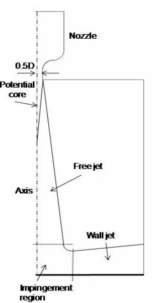
Fig. 1.1 Definition schematic of an axisymmetric impinging jet ... 2

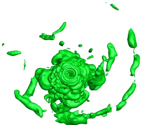
Fig. 1.2 Iso-surfaces of λ2 criterion colored with velocity magnitude contours close to the nozzle exit ... 4

Fig. 1.3 Iso-surface of pressure contours (-20 pa) (top view) ... 4

Fig. 1.4 Typical boiling curve and associated boiling regimes (Coursey, 2007) . 10 Fig. 2.1 Definition schematic of an impinging circular jet with large height-to-diameter ratio (adapted from Rajaratnam et al. (2010)) ... 18

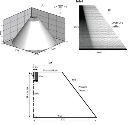
Fig. 2.2 (a) Full 3D geometry, (b) cross-section of the computational domain and mesh, and (c) domain dimensions and boundary conditions ... 21

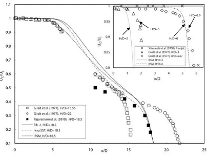
Fig. 2.3 Comparison between computational and experimental centreline velocity ... 26

Fig. 2.4 Mean velocity distribution at different x/H stations, comparing experimental data and CFD results; (a) H/D = 2, (b) H/D = 6, (c) H/D = 18.5 ... 31

Fig. 2.5 Comparison of experiments and CFD for the shear stress profiles uv /U_j2 at different x/H stations and H/D ratios ... 33

Fig. 2.6 Wall shear stress along the impingement plate ... 36

Fig. 2.7 Static pressure along the impingement plate ... 37

Fig. 2.8 Radial velocity V/Vm at different r/D stations in the wall jet ... 39

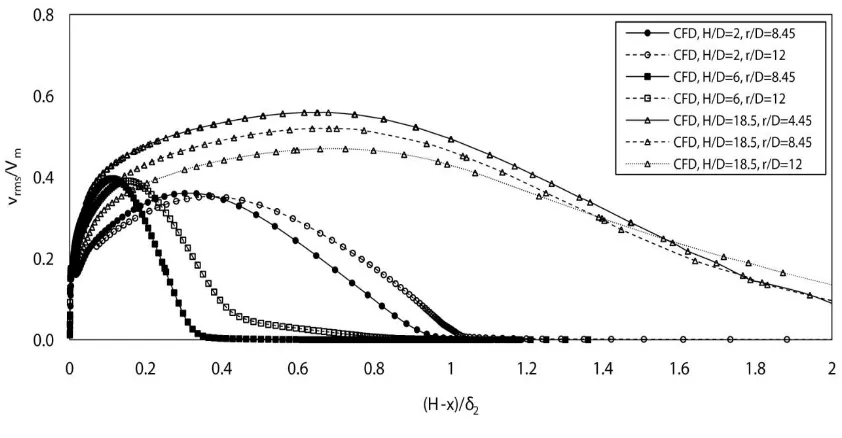
Fig. 2.9 Comparison of vrms/Vm for different nozzle heights, at different r/D stations in the wall jet region (fully developed) ... 40

Fig. 2.10 Comparison of uv /Vm2 for different nozzle heights, at different r/D stations in the wall jet region (fully developed) ... 41

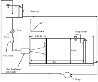
xiv Fig. 3.1 Impinging jet experimental setup (Roussinova and Balachandar, 2012) 51

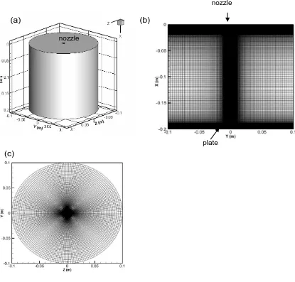
Fig. 3.2 Cross-section of the mesh in the nozzle ... 52

Fig. 3.3(a) Virtual tank dimensions, (b) cross-section of the mesh inside the tank,

(c) cross-section of the mesh on the plate ... 54

Fig. 3.4 Mesh requirement analysis ... 56

Fig. 3.5 Comparison of mesh cell size with the Kolmogorov length scale at r/D=0

... 57

Fig. 3.6 Comparison of (a) mean axial velocity, (b) turbulent axial velocity,

obtained from LES and PIV experiments (Tandalam et al. 2010) at x/D = 1 ... 60

Fig. 3.7 Mean centreline velocity obtained from LES, RANS and experiments .. 62

Fig. 3.8(a) Mean static pressure along the wall, (b) mean wall shear stress ... 63

Fig. 3.9 Turbulence intensities obtained from LES and experiments ... 64

Fig. 3.10(a) Mean radial velocity profiles (V/Uj), (b) turbulent velocity profiles

(vrms/Uj) in wall region, at different r/D stations ... 65

Fig. 3.11 Contours of (a,b) mean velocity magnitude superimposed with sectional

streamlines, (c,d) streamwise turbulent velocity fluctuations and (e,f) shear stress

in the whole domain and close to the plate ... 67

Fig.3.12 Iso-surfaces of a) λ2 criterion colored with velocity magnitude contours,

b) static pressure (-20 Pa) colored with vorticity magnitude contours ... 70

Fig. 3.13 Deformation of shear layer in y-z plane visualized by the instantaneous

vorticity magnitude contours at (a) x/D = 1, (b) x/D = 1.25, (c) x/D = 1.5, (d) x/D

=1.75, (e) x/D = 2, (f) x/D = 4, (g) x/D = 7, (h) x/D = 15, (i) x/D = 20 ... 72

Fig. 3.14 (a) History of static pressure, (b) power spectra at x/D = 2 and r/D = 0.5

xv Fig. 3.15(a) History of static pressure, (b) power spectra at x/D = 18 and r/D = 5

... 75

Fig. 3.16 Instantaneous velocity magnitude (y-z plane) and static pressure

contours (x-y and x-z planes) with sectional streamlines over the characteristic

period (T2), (a) t/T2 = 0, (b) t/T2 = 1/5, (c) t/T2 = 2/5, (d) t/T2 = 3/5, (e) t/T2 = 4/5 and

(f) t/T2 = 5/5 (the red circle in y-z plane shows the nozzle) ... 78

Fig. 3.17 Generation of secondary vortices in the wall region ... 81

Fig. 3.18 Instantaneous sectional streamlines and (black) and mean (red) wall

shear stress in x-y plan over the characteristic period (T2), (a,b) t/T2 = 0, (c,d) t/T2

= 1/5, (e,f) t/T2 = 2/5, (g,h) t/T2 = 3/5, (i,j) t/T2 = 4/5 and (k,l) t/T2 = 5/5 ... 83

Fig. 4.1 Boiling model algorithm ... 102

Fig. 4.2 Implementation of breakup, coalescence and IAC equation in

OpenFOAM ... 104

Fig. 4.3 k − ε turbulence model, modified to account for gas bubbles ... 106

Fig. 4.4 a) Schematic of a two-phase pipe flow (not to scale), b) 2D axisymmetric

mesh ... 108

Fig. 4.5 Radial distribution of a) interfacial area concentration, b) void fraction, c)

liquid velocity, d) bubble diameter ... 111

Fig. 4.6 Sketch of the DEBORA test setup (Garnier et al. 2001) ... 113

Fig. 4.7 Radial distribution of a) liquid temperature, b) interfacial area

concentration, c) void fraction, d) bubble diameter ... 115

Fig. 4.8 a) Computational domain, b) mesh for the impinging jet ... 117

Fig. 4.9 Boiling curve obtained from current CFD analysis, simulation of

Narumanchi et al. (2008) and experiment of Katto and Kunihiro (1973) ... 119

xvi Fig. 4.11 Profiles at different radial stations; a) IAC, b) void fraction, c) liquid

xvii LIST OF TABLES

Table 3.1 Grid data (virtual tank) ... 55

xviii NOMENCLATURE

A_b Area covered by nucleation bubbles

As Surface area of the wall per unit volume

A _w Contact area with the wall per unit volume

C_D Drag force coefficient

C_L Lift force coefficient

C_hl Liquid Stanton number

C_pl Specific heat of liquid

Cf Fanning friction number

C_WL Wall lubrication force coefficient

dB Bubble detachment diameter

dref Reference diameter of bubbles

D Nozzle diameter

f Bubble detachment frequency

F Force

F _gL _{Lift force}

F _gWL _{Wall lubrication force}

F gTD Turbulent dispersion force

F gVM Virtual mass force

F _gD _{Drag force}

g Gravity acceleration

hC Convection heat transfer coefficient

h_sat Saturation enthalpy of liquid

h_g Enthalpy of gas phase

hk Specific enthalpy of phase k

hl Enthalpy of liquid

H Nozzle height

IAC Interfacial area concentration

N_w Site density of bubbles

p Pressure

P_s Stagnation point pressure

qt_k Turbulent heat flux

q w Wall heat flux density

qW Total heat flux from the wall

Q_E Evaporative heat flux

QC Convective heat flux

Qk Heat flux

Q_Q Quenching heat flux

r_1/2 Jet half width

Rk Diffusion of phase k

xix

Re Reynolds number

t Time

t_w Bubble waiting time

T₁ Time period for roll up vortices close to the nozzle

T₂ Time period for large scale structures hitting the plate

Tw Wall temperature

Tl Liquid temperature

Tsat ,l Saturation temperature of liquid

u_τ Shear velocity

uu

Normal stress in x direction

vv

Normal stress in y direction

uu

Normal stress in z direction

uv

Shear stress in x-y plane

uw

Shear stress in x-z plane

vw

Shear stress in y-z plane

Uj Jet exit velocity

Uc Jet centreline velocity

Um Jet radial maximum velocity

U

_k Velocity of phase k

Greek symbols

δ2 Distance above the plate at which V = 0.5Vm

ρ_k Density of phase k

k Turbulent kinetic energy

ε Turbulent dissipation rate

ν Kinematic viscosity

ω Specific turbulent dissipation rate

θ Circumferential direction

η Kolmogorov length scale

Δ Grid size

τ_ij Subgrid-scale stresses

αk Void fraction of phase k

Γki Phase change from phase k to i

Γ_ik Phase change from phase i to k

k_l Heat conductivity of liquid

ΔT_sub Subcooling temperature

ΔT_sup Superheat temperature

∅C _{Source term for bubble coalescence}

∅B _{Source term for bubble breakup}

∅nuc _{Source term for bubble nucleation}

μmol _{Molecular viscosity}

μbubble Bubble induced viscosity

1 CHAPTER 1

2 1.1. Background and motivation

Turbulent jets impinging on a flat surface are commonly used in many

industrial applications where enhancement of heat and mass transfer is required.

Examples of such applications include cooling, heating, cleaning and drying. In

this type of flow, the flow field is a combination of several distinct features, such

as a free jet, a stagnation flow, and a radial wall jet (see Fig. 1.1). Each of these

flows has its own particular characteristics which have gained the attention of

many researchers.

3

1.1.1. Adiabatic round impinging jets

The characteristics of round impinging jets strongly depend upon several

parameters such as Reynolds number, distance between the nozzle and the

plate, nozzle geometry and the rate of turbulence introduced at the inlet to the

domain (Manceau et al. 2014).

The core of the free jet is surrounded by a growing shear layer. In this

shear layer the development of the Kelvin-Helmholtz instabilities results in the

formation of ring vortices. Yule (1978) defined the term ―vortex‖ as a part of a

flow field accompanying a concentrated, continuous, coherent distribution of

vorticity which is uniform in the direction of the vorticity vector. With increasing

downstream distance the ring vortices change into large eddies. An eddy may be

described as a vorticity containing region of fluid which can be identified as a

moving coherent structure in the flow (Yule, 1978). These eddies are significant

features of the turbulent region of the jet. However, features like

three-dimensionality and irregularity of the vorticity field restrict us fromdenoting them

as a ring vortex.

The ring vortices which change into large eddies (see Figs. 1.2 and 1.3)

have a three-dimensional shape and have lost their axisymmetric behaviour.

These eddies influence the flow field and cause pressure fluctuations on the

plate (Hadziabdic and Hanjalic, 2008). This phenomenon causes an unsteady

behaviour in the radial distributions ofwall shear stress and wall pressure and will

eventually influence the rate of the heat transfer from the plate (Hall and Ewing,

4 unsteady structures impinging on the plate. These impinging unsteady structures

cause separation and reattachment of the flow in the wall region which are

associated with variations in the wall shear stress (El Hassan et al. 2013).

Fig. 1.2 Iso-surfaces of λ2 criterion colored with velocity magnitude contours

close to the nozzle exit

5 The jet exit mean velocity remains constant inside the core part of the free

jet region, where the turbulence intensity is very low. Once the core reaches its

maximum penetration, which is associated with an increase in turbulence

intensity, a sharp decay in the jet centreline velocity occurs. Basically,

penetration of the turbulence from the shear layer to the core part of the jet

destroys the jet and results in a large decay in jet streamwise velocity. In the

impinging zone, the flow loses its axial velocity and changes direction due to the

presence of the plate. A wall jet is formed on the plate and attains a fully

developed behaviour as it travels towards the downstream.

There are many numerical and experimental studies in the literature on

different aspects of impinging jets. These analyses include investigations on the

steady and unsteady flow parameters, effect of nozzle stand-off distance,

behaviour of wall shear stress, pressure distribution and also separation and

reattachment of flow along the wall jet zone.

On the experimental side, the work carried out by Yule (1978) has been of

particular interest to researchers because of its fundamental overview on the

physics of impinging jets. Yule (1978) showed that for impinging jets with large

distance between the nozzle and the plate, large eddies have a wide range of

sizes and trajectories with no symmetry between them. This phenomenon results

in an unsteady three-dimensional behaviour of large scale structures causing

pressure fluctuation in the impinging zone.

The effect of nozzle stand-off distance on flow parameters has been

6 classified impinging jets with H/D > 8.3 into three sub-regions including free jet,

impinging region and wall jet zone as shown in Fig. 1.1. Following this, Giralt et

al. (1977) conducted experiments on axisymmetric turbulent impinging jets for 3

< H/D < 25. They developed an experimental correlation between flow

parameters and different H/D ratios. Although their study covered different H/D

cases, it was limited to a mean value analysis and did not present any time

history of the data.

Another aspect of impinging jetswhich has been investigated by different

researchers is the behaviour of wall shear stress and static pressure in different

flow configuration. Bradshaw and Love (1961) measured velocity, wall static

pressure and skin friction for a case with H/D = 2. They observed that the high

pressure region on the plate is slightly larger than the diameter of the jet. The

peak of the wall skin friction magnitude occurred at a radius equal to that of the

jet. A study carried out by Deshpande and Vaishnav (1982) showed a decreasing

trend for the wall shear stress as the nozzle stand-off distance increases. Recent

unsteady analysis of El Hassan et al. (2013) on the wall shear stress using

particle image velocimetry showed significant influence of large-scale vortical

structures on the wall shear stress (Re = 1260, H/D = 2). The influences of the

vortex ring, the secondary and the tertiary vortices were reported to be the main

mechanisms involved in the wall shear stress variation.

On the numerical side, there are different Reynolds-Averaged

Navier-Stokes (RANS) analyses as well as Large Eddy Simulations (LES) and Direct

7 of the studies are focused on the challenges associated with the turbulence

modeling of impinging jets.

The research of Craft et al. (1993) is one of the fundamental RANS

studies on impinging jets which investigates the issues with the turbulence

modeling for this type of flow. The benchmarking of the simulations was

performed using the experimental results of Cooper et al. (1993). Their study

suggested the higher performance of the Reynolds Stress Model with the wall

reflection models compared to other turbulence models.

Due to the limitations associated with LES and DNS computations, most

of these studies deal with small H/D ratios. Olsson and Fuchs (1998) performed

large eddy simulations for a case with H/D = 4. The purpose of their simulations

was to study the turbulence parameters and the dynamic behaviour of impinging

jets. They noticed generation of secondary vortices in the wall jet region which

was found to be a result of primary vortices generated at the jet exit shear layer.

They also observed that the primary vortices do not have an axisymmetric shape

when approaching the plate.

Hadziabdic and Hanjalic (2008) used LES to analyze a circular impinging

jet at Re = 20,000 and H/D = 2. The case that they analyzed showed that due to

the small distance between the nozzle and the plate, the generated vortices are

short-lived and undergo a faster stretching breakdown than in a free jet due to

the radial deflection. They also noticed that because of the jet flapping, the

stagnation point meanders in time around the jet geometrical centre. They

8 was due to the reattachment of the recirculation bubble and associated

turbulence production.

Uddin et al. (2013) used LES to model impinging jets at two Reynolds

numbers of 13,000 and 23,000 at H/D = 2, in order to extract the reason for the

second peak observed in the radial distribution of the Nusselt number profile.

They found that the flow acceleration in the developing region of the boundary

layer is closely related to the secondary peak in the radial distribution of Nusselt

number.

Wu and Piomelli (2014) performed LES to study the roughness effects on

the evolution of azimuthal vortices in impinging jets with H/D = 1 and Re =

66,000. They modeled one case with laminar inflow and another one with

turbulent inflow conditions. They observed a wider and weaker wall jet for the

rough surface compared to the smooth surface for the turbulent case. They

noticed that the peak of the velocity profile on the wall jet was shifted away from

the plate. They concluded that roughness results in transition to the turbulence

regime even if the inlet jet is laminar.

1.1.2. Round impinging jets with boiling heat transfer

One of the important applications of impinging jets in industry is their

usage in removal ofalarge amount of heat from a surface. For example,

impinging jets are used to cool electronic components in the computer industry

and to dissipate the heat in pistons in the automotive industry. Boiling heat

9 reduces the heat transfer, which could allow the wall temperature to increase to

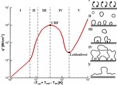
the burnout point. Boiling heat transfer is characterized by a curve with different

regimes, as shown in Fig. 1.4. In Regime I, due to the small temperature

difference between the wall and liquid (wall superheat), the heat transfer

mechanism is only through free convection. This single-phase heat transfer

problem can be treated using common analytical solutions for free convection.

The nucleate boiling regime, which is characterized by two sub-regimes (II and

III), begins once bubbles are generated on the surface. Regime II refers to the

condition when the isolated bubbles are formed at their own nucleation sites

without interacting with each other when departing the surface. At higher wall

superheat (Regime III), bubbles coalesce at different directionsas a consequence

of higher nucleation frequency. Further increase of the wall superheat causes the

boiling curve to rise to the local maximum heat flux point, called the critical heat

flux (CHF). At this stage the high generation of vapor compared to previous

stages results in a blockage between the surface and liquid. Therefore, heat

must be transported through the vapor layer which is less efficient and results in

a reduction in the heat flux. In the design of appliances working with boiling heat

transfer, the CHF point is defined as a thermal limit in which further increase of

10 Fig. 1.4 Typical boiling curve and associated boiling regimes (Coursey, 2007)

The transition boiling regime (Regime IV) occurs after the CHF point,

characterized by increasing wall temperature while the heat flux removal

decreases. This is due to the increase of bubbles generated on the surface (dry

area). Therefore, this regime is not known to present any practical applications.

Finally, following the transition regime, the boiling curve reaches a local minimum

point denoted as the Leidenfrost point. At this point, the surface enters the

film-boiling regime (V). In this regime, in order to transfer heat to the liquid, it must be

conducted across a continuous vapor film. This regime of heat transfer is an

inefficient processand is not recommended for cooling purposes. It results in high

11 There are a number of studies in literature on the numerical modeling of

subcooled boiling. Basically, most of these studies deal with the challenges of

numerically modeling the boiling phenomenon and correlating it with the

experimental results.In this regard, the model developed at Rensselaer

Polytechnic Institute (RPI) by Kurul and Podowski (1990, 1991) has gained

significant attention. According to the RPI model, the boiling heat transfer is

divided into three components; convective, quenching and evaporative heat

fluxes. The convective part provides for single-phase convection, quenching

refers to liquid filling the wall vicinity after bubble detachment due to vaporization

and the evaporative component is for the fluid that evaporates.

The numerical simulation of boiling heat transfer is performed by

employing different two-phase flow methods. The Eulerian-Eulerian and Volume

of Fluid (VOF) approaches are widely used for this purpose. The

Eulerian-Eulerian method is more accurate because it solves the balance equations of

mass, momentum and energy for both phases separately. However, it is

computationally more expensive. The coupling of two phases is carried out by

introducing source/sink terms such as interfacial forces and heat flux in these

equations.

Krepper and Rzehak (2011) used the Eulerian-Eulerian approach in CFX

software for modeling the boiling heat transfer in a pipe flow. Most of their results

showed good agreement with the experimental results, except for the bubble size

radial distribution. Evaluation of their model shows that there is no interfacial area

12 changes in the bubble size and takes into account the effect of bubble break-up

and coalescence in the model. In their recent study, Krepper et al. (2013)

updated their model by implementing a population balance method which takes

into account the variation of bubble size due to bubble breakup/coalescence and

condensation/evaporation processes. The quality of their results was significantly

improved, especially for the bubble size distribution.

Michta (2011) and Michta et al. (2012) used OpenFOAM to model the

boiling heat transfer in a pipe flow and considered the IAC equation as well as

different interfacial forces in the model. The choice of OpenFOAM was based on

the fact that it is an open source code and gives permission to the user to modify

the code and to incorporate the appropriate experimental correlations. They

found reasonable results in the adiabatic part of their code, however, for the

boiling part the results were not in a good agreement with the experiments.

Kunkelmann and Stephan (2010) simulated the nucleate boiling heat

transfer using the Volume of Fluid (VOF) method in OpenFOAM. The boiling of a

single bubble was simulated by modifying the OpenFOAM default solver. Their

model captured the growth, departure and movement of the bubble. Good

agreement with the experimental results was observed for the bubble size as well

as the mean wall superheat.

There are several different interfacial forces acting on both the continuum

and dispersed phases in two-phase flows. They include, drag, lift, wall

lubrication, turbulent dispersion and added mass forces. In order to properly

13 the bubbles in two-phase flow simulations, different correlations have been

suggested by different researchers. Drag is one of the primary interfacial forces

which is generated by the continuous phase on the dispersed phase due to the

movement of the dispersed phase. The correlation developed by Ishii and Zuber

(1979) has been widely used for modelling the effect of the drag force. Tomiyama

et al. (2002) measured trajectories of single air bubbles in simple shear flow to

determine the transverse lift force acting on single bubbles. Their correlation has

gained a lot of attention in the literature for modelling the lift force in two-phase

flows. Antal et al. (1991) was the first to develop an analytical expression for the

wall lubrication force. This is a repulsive force generated by the wall which

pushes the bubbles away from it. Later, Tomiyama (1988) improved this model to

pipe geometries. Frank (2005) upgraded the Tomiyama (1998) wall lubrication

force coefficient and made it independent of the geometry. The virtual mass force

which is generated due to the relative acceleration of one phase to the other is

another important interfacial force. The correlation developed by Zuber (1964)

has been widely used for the virtual mass force by many researchers.

Narumanchi et al. (2008) developed a numerical model for boiling heat

transfer in an impinging jet. The application of their study was in the cooling of

power electronic components. They employed the Eulerian-Eulerian approach in

Fluent software and found reasonable results for the prediction of wall superheat

in the stagnation point region. However, no information was provided about the

14 Abishek et al. (2013) numerically studied the effect of heater-nozzle ratio

on the boiling phenomenon in an impinging jet. The jet Reynolds number was

2,500 with a subcooling of 20°C. They used the RPI model for decomposing the

heat flux on the impingement plate and RNG k-ε to model the turbulence. The

Eulerian-Eulerian two-phase flow model was used for the simulation. They found

that irrespective of the heater-nozzle size ratio, at high superheat temperatures

the quenching heat flux contributes to the major part of the heat flux. They also

developed a correlation for the heat flux as a function of wall superheat and the

size of the heater.

1.1.3. Objectives and outline of the dissertation

As the literature shows, there are many numerical and experimental

simulations to study the various aspects of impinging jets. On the experimental

side, detailed unsteady analysis of flow structures seem to be limited. On the

numerical side, most of the unsteady studies are either RANS based or only

cover small stand-off distances (H/D < 4).

In the first phase of this dissertation (Chapter 2), the mean value analysis

is carried out on impinging jets to evaluate the effect of nozzle stand-off distance

on different mean flow parameters. In this regard, Reynolds-Averaged

Navier-Stokes simulations are carried out using different turbulence models at three

nozzle height-to-diameter (H/D) ratios.

In the second phase (Chapter 3), due to the limited reporting of unsteady

15 flow features at large nozzle height-to-diameter ratios. The objective is to answer

critical questions raised by the steady analysis in Chapter 2. In this regard, an

unsteady simulation using Large Eddy Simulation (LES) is carried out on an

impinging jet with H/D = 20.

Commercial software has limitations in implementing the appropriate

experimental correlations for every simulation, Furthermore, due to the

inaccuracy observed in the previous numerical simulations of boiling heat

transfer, it is of interest to develop a CFD code to simulate the boiling heat

transfer for an impinging jet. As the literature shows, previous CFD approaches

for boiling simulation in impinging jets do not take into account all aspects of

two-phase flow phenomenon, particularly in the boiling part of the model. In this

regard, adetailed Eulerian-Eulerian two-phase flow model was developed using

the open source codeOpenFOAM, which takes into account the effects of

interfacial forces, breakup/coalescence of the bubbles as well as the interfacial

area concentration (IAC) equation (chapter 4). It is expected that the model

developed in this dissertation presents more accurate results than previous

investigations and advances the state-of-the-art research on boiling simulation

16 CHAPTER 2

RANS ANALYSIS OF THE EFFECT OF NOZZLE STAND-OFF DISTANCE

17 2.1. Introduction

Reynolds-Averaged Navier-Stokes (RANS) simulations have been carried

out on turbulent impinging jets to evaluate the effect of nozzle height-to-diameter

ratio on different flow parameters. In this regard, three cases with different H/D

ratios have been selected for the simulations, corresponding to short (H/D = 2),

intermediate (H/D = 6) and long (H/D = 18.5) jets.

Circular jets impinging vertically on flat surfaces have many practical

applications such as in heating, cooling, metal cutting, fabric weaving and

cleaning. Most of the experiments on impinging jets have been performed for

short stand-off distances, i.e., with an impingement height (H) to nozzle diameter

(D) ratio of less than six. Cooper et al. (1993) carried out experiments on a jet

impinging on a large plane surface and measured mean and turbulence

quantities in different regions of the jet. They considered two Reynolds numbers,

23,000 and 70,000, while the H/D ratio varied from two to ten, with particular

focus between two and six. For H/D < 6, researchers have found that the core of

the jet is still developing when reaching the plate surface (Nishino et al. 1996;

Hadziabdic and Hanjalic 2008, Shademan et al. 2013).

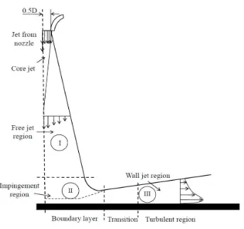
For larger impingement heights (H/D > 8.3), Beltaos and Rajaratnam

(1974, 1977) classified the flow into three different regions: the free jet portion

(region I), the impingement zone (region II) and the axisymmetric wall jet portion

(region III), as illustrated in Fig. 2.1.Giralt et al. (1977) conducted experiments on

18 34,000 up to 80,000. Based on their experimental data, they developed a

conceptual model for submerged, axisymmetric, turbulent impinging jets, which

can be used to analyze the effect of increasing the nozzle distance from the

plate. Recently, Rajaratnam et al. (2010) performed measurements on an

impinging jet with a large H/D ratio of 18.5 at Re = 100,000 using a standard

constant temperature hot-wire anemometer and evaluated the mean and

turbulence characteristics in regions I and II. They noticed self-similarity in the

radial distribution of mean velocity profiles up to regions close to the

impingement zone.

Fig. 2.1 Definition schematic of an impinging circular jet with large

19 Numerical simulation of a round jet impinging on a flat surface using

Reynolds-Averaged Navier-Stokes (RANS) turbulence models have been the

subject of considerable research, forming part of the 2nd ERCOFTAC-IAHR

Workshop on Refined Flow Modelling in 1993. Subsequently, Craft et al. (1993)

published their research using different turbulence models to analyze the heat

transfer in the impingement region of the jet, i.e., region II. They observed that

the results were not in good agreement with experimental data and attributed this

to the weakness associated with the eddy viscosity stress-strain relationship in

the turbulence models used. They also implemented second-moment closure

models. Due to the incorrect response of the wall reflection process, the eddy

viscosity model (k - ε) and the basic Reynolds Stress Model (RSM) failed to

produce reasonable results. However, an improved RSM which takes into

account the wall reflection effects generated satisfactory results.

Most of the previous analyses of impinging jets deal with a specific nozzle

stand-off distance. As mentioned earlier, the experiments by Giralt et al. (1977)

were carried out to study the effect of stand-off distance, but the evaluation is

limited to the quantities inside the jet, the variation of turbulence intensity along

the jet axis and presentation of a numerical model for determining the wall shear

stress. There is a lack of information regarding the effect of impingement

distance on the mean and turbulence quantities in different regions of the

impinging jet, including the free jet portion, impinging zone and the wall jet

region. The focus of the current study is to investigate the mean and turbulence

20 values. In addition, it is also of practical interest to evaluate the mean and

turbulence quantities in regions very close to the wall because of the

uncertainties associated with the experimental techniques in this region.

In this chapter, three-dimensional RANS simulations have been carried

out for H/D = 2, 6 and 18.5 at Re = 100,000. H/D = 2 represents a jet with

impingement occurring in the potential core region. Jets with H/D = 6 are in a

transitional state and the core of the jet is almost fully penetrated by the external

flow. At H/D = 18.5, the jet can be considered as fully developed with distinct

regions of flow including potential core, free jet and impingement zone. The

experiments performed by Rajaratnam et al. (2010) have been used as the

primary benchmark to validate the numerical model. However, other

experimental data from Bradshaw and Love (1961) and Giralt et al. (1977) are

also used to assess the accuracy of the computational results.

2.2. Numerical method

2.2.1. Geometry modelling and boundary conditions

In this research, a high velocity air jet exiting from a circular nozzle

impinges vertically on a flat plate and spreads out as a radial wall jet. The nozzle

has an exit diameter of D = 23.4 mm. The stand-off distances between the nozzle

exit plane and the plate are H = 46.8 mm (H/D = 2), 140.4 mm (H/D = 6) and 432

mm (H/D = 18.5). The value H/D = 18.5 is specifically chosen to match the

21 normal to the plate. Details of the computational domain and mesh generated for

the current simulations are shown in Fig. 2.2.

Fig. 2.2 (a) Full 3D geometry, (b) cross-section of the computational domain and

mesh, and (c) domain dimensions and boundary conditions

The full 3D geometry for the H/D = 18.5 case is illustrated in Fig. 2.2a and the

structured mesh system and half cross-section of the domain with the boundary Inlet

22 conditions applied in the numerical model are shown in Figs. 2.2b and 2.2c,

respectively. In Fig. 2.2c, the jet is aligned with the x-axis and r is the radial

distance from the x-axis. To ensure that the location of the outlet boundary has

negligible influence on the pressure and velocity fields, the computational domain

is taken to have a radius of 0.4 m (17D) along the plate. Shorter distances

between the pressure outlet boundary and the jet axis were taken for the H/D = 2

and 6 cases, but sufficiently long enough to minimize the influence of this

boundary on the flow field.

A constant velocity of 61m/s is imposed at the inlet, corresponding to a

Reynolds number of 100,000 based on the nozzle exit velocity and diameter.

Since the air escapes to the atmosphere through the side and top boundaries of

the computational domain, they are set as pressure outlets. The plate is

considered to be a no-slip boundary. The Low Reynolds Number Modelling

(LRNM) method (Launder and Spalding, 1974) is used as a numerical model to

accurately capture the wall effect.

In order to provide a fine mesh with minimal skewness in the boundary

layer near the impinging wall, the mesh system is constructed of hexahedral

elements. A high-density mesh, as shown in Fig. 2.2b, is used to capture the high

shear stresses within the jet, as well as those generated near the plate,

particularly in the impingement zone. For the rest of the domain, where the wall

effect is smaller, a coarser mesh is used. Different mesh schemes, including fully

structured, fully unstructured and hybrid meshes with different numbers of cells

23 results, the fully structured mesh was chosen for all subsequent simulations. Grid

independence tests were also performed, the grid size being increased in 20%

increments until no noticeable variance in the drag force exerted on the plate was

observed. The total number of cells required to ensure a grid independent

solution from the current simulations was approximately 1.1 x 106 for H/D = 2,

1.38 x 106 for H/D = 6 and 1.84 x 106 for H/D = 18.5.

2.2.2. Governing equations

The impinging jet flow is modeled by the steady 3D incompressible RANS

equations, representing conservation of mass and momentum balance. These

equations, in tensor form, are:

∂u i

∂x_j = 0 (2.1)

∂

∂x_j u iu j = ∂ ∂x_j ν(

∂u i

∂x_j + ∂u j

∂x_i) − 1 ρ

∂p ∂x_i−

∂uiuj

∂x_j (2.2)

where

x

, u

, u

′, p, ρ

ν

fluctuations, pressure, density and kinematic viscosity, respectively, and the

over-bar indicates a time-averaged quantity (Hoffmann and Chiang, 2000).

Cooper et al. (1993) has reported that for the simulation of impinging jets,

the k - ε model over-predicts the turbulent kinetic energy near the stagnation

point. In order to reduce this effect, different turbulence models, which take into

24

The Realizable k – ε model (Shih et al. 1995), the k - ω SST (Shear Stress

Transport) model (Menter, 1994) and the Reynolds Stress Model (RSM)

(Launder et al. 1975) have been implemented in the current simulations. For the

Realizable k - ε model, the LRNM is used.The k - ω SST turbulence model takes

into account the low-Re effects in the flow. In the SST version of the model, the

standard k – ω model is used for the near-wall region, combined with a standard

k – ε model in the fully turbulent zone (Menter, 1994). The Reynolds Stress

Model (RSM), which is also used in this study, takes into consideration

multi-scale and anisotropic effects of turbulence. In RSM, a transport equation is

solved for each of the unknown stresses in the Reynolds stress tensor. A wall

reflection scheme and pressure gradient terms are included in the model

(Launder et al.1975). The details of these models can be found in FLUENT

6.3.26 User’s Guide.

The finite volume method is used to discretize the governing equations,

with the QUICK scheme for discretization of the convective terms. The Standard

scheme for the pressure interpolation is used. For the pressure-velocity coupling,

the SIMPLE algorithm developed by Patankar and Spalding (1972) has been

applied. FLUENT 6.3.26 is used to solve the discretized governing equations.

During the simulations the drag force exerted on the plate was monitored, and

the solution was considered converged when no significant change in drag was

observed (changes less than the order of 10-3). For all results presented in this

chapter, the residuals of the continuity, momentum and turbulence equations are

25 2.3. Results

To understand the effect of the nozzle height on the behaviour of

impinging jets, different mean and turbulent flow parameters have been analyzed

at various H/D ratios. These quantities include the decay of centreline velocity,

radial distribution of axial velocity, pressure and shear stress distribution along

the plate, and mean and root mean square (rms) velocities in the wall jet region.

2.3.1. Centreline velocity

To validate the current CFD simulations, the results are compared with the

available experimental data of Giralt et al. (1977) and Rajaratnam et al. (2010).

Although there are three distinct cases in the current simulations (H/D = 2, 6 and

18.5), for the purpose of identifying the best RANS turbulence model to use for

subsequent analysis, only the H/D =18.5 case was selected for a detailed

comparison. According to the results shown in Fig. 2.3, the Realizable k - ε and

RSM models show some over-prediction of the centreline velocity entering the

impingement zone, but recover to provide a close match to the data of

Rajaratnam et al. (2010) near the plate surface. On the other hand, the k - ω SST

model provides a good agreement with the data of Rajaratnam et al. (2010)

through the impingement zone and very close to the plate. Note that k - ω SST

26 Fig. 2.3 Comparison between computational and experimental centreline velocity

All three models show good agreement with the H/D = 18.5 experimental

data of Rajaratnam et al. (2010) as the flow approaches the plate (region II), but

Fig. 2.3 also shows that RSM yields more accurate centreline velocity in the free

jet (region I). Based on this comparison, and also considering that RSM is a

non-isotropic turbulence model, the RSM was selected as the main turbulence model

for further simulations in all H/D cases. The following sections investigate the

variation of the centreline velocity as the H/D ratio increases from 2 to 18.5.

H/D=2

H/D=3

H/D=6

27

2.3.1.1. H/D = 2

The case of H/D < 6 represents an impinging jet where the core of the jet

reaches the plate and has not yet been fully penetrated by the ambient flow. No

fully developed free jet region exists for this type of impinging jet and different

regimes of the jet are not distinguishable. To obtain a better understanding of this

kind of impinging jet, H/D = 2 was chosen for the current CFD study and the

results are compared with the available experimental data of Giralt et al. (1977)

at H/D = 3 (see inset in Fig. 2.3). This comparison confirms that the current

results follow the expected trend. For H/D = 2, no significant decay in the

centreline velocity between the nozzle and the plate is observed, except in the

impinging zone which starts around x/D = 1 and extends to the stagnation point.

2.3.1.2. H/D = 6

As previously discussed, H/D = 6 represents an intermediate regime of an

impinging jet in which the core of the jet has reached the maximum penetration

(Beltaos and Rajaratnam, 1977). Therefore, the current CFD analysis was

carried out at H/D = 6 and the results are compared with the experimental data of

Giralt et al. (1977) at H/D = 6.67 and the free jet results of Shinneeb et al. (2008)

(see inset in Fig. 2.3). Similar to H/D = 2, at H/D = 6 no decay in the centreline

velocity is observed up to the impinging zone (i.e., 0 <x/D < 5), which confirms

that the core of the jet is still developing up to a location very close to the plate.

28 is influenced by the impingement wallfor x/D > 5. Results for the radial

distribution of the axial velocity are discussed in Section 2.3.2.

2.3.1.3. H/D = 18.5

According to the literature discussed above and also based on the results

shown in Fig. 2.3, H/D = 18.5 represents an impinging jet in which all three

sub-regions of an impinging jet co-exist, namely the free jet region, impingement zone

and wall jet region. Figure 2.3 shows that for H/D = 18.5, the core of the jet is still

developing up to about x/D = 6and no decay in the centreline velocity can be

observed. For x/D > 6, the free jet region starts to develop and a large decay in

centreline velocity occurs up to about x/D = 15 as the ambient flow is entrained

with the jet. For x/D > 15, the flow senses the plate and a much sharper decay in

the centreline velocity can be seen compared to the decay in the region 6 < x/D <

15. This is due to the transfer of the momentum from the axial to the radial

direction.

One can note from Fig. 2.3 that the results of Rajaratnam et al. (2010)

deviate significantly from the results of the present simulations and the

experimental results of Giralt et al. (1977) for x/D < 14. It is important to recall

that the design of the nozzle has an impact on the downstream evolution of the

jet (Xu and Antonia, 2002). The shape of the nozzle affects the behaviour of the

shear layer at the jet exit, influencing flow characteristics such as jet expansion in

29 impingement zone. This could be the reason for this discrepancy. Nevertheless,

for x/D > 17, where the flow approaches the impingement point, the mean values

of the streamwisecentreline velocity obtained from the CFD calculations (H/D =

18.5) match very well with the measurements of Rajaratnam et al. (2010), and

fall between the results of Giralt et al. (1977) corresponding to H/D = 15.6 and

H/D = 22.

2.3.2. Radial distribution of velocity

Figure 2.4 illustrates the effect of H/D on the radial distribution of the

streamwise mean velocity, normalized by the local maximum value Um, for

locations near the impingement plate (0.785 < x/H < 0.99). The radial distance is

normalized by the jet half-width δ1, defined as the radial location where U =

0.5Um.

For H/D = 2, Fig. 2.4a shows that there is a slight shift in the peak of the

streamwise velocity profiles towards the axis when moving from x/H = 0.785 to

0.93. This phenomenon confirms that the flow is still accelerating and results in a

transfer of momentum from the axial to radial direction in the region 0.785 < x/H

<0.93. For the rest of the axial stations x/H = 0.97, 0.98 and 0.99, the streamwise

velocity profiles collapse on each other.

In Fig. 2.4b the streamwise velocity profiles at several axial stations are

plotted for H/D = 6. The flat shape of the profile (no decay in the centreline

30 minor losses) has retained its top-hat shape up to this station. The peak

observed in the other profiles is located off the centreline, which confirms that the

flow has started to change direction from axial to radial. Comparison of the jet

diameter at similar axial stations for H/D = 2 and H/D = 6 (Figs. 2.4a and 2.4b)

shows a decrease in this value as the H/D ratio increases.

The velocity profiles at stations very close to the plate (x/H = 0.98 and

0.99) bring out another important difference between the H/D = 2 and 6 cases.

Note that due to limitations in experimental techniques, measurements in regions

very close to the plate are susceptible to large uncertainties. Figure 2.4a

illustrates that there is a collapse in the velocity profiles at these stations for H/D

= 2, which suggests that the flow has changed direction before these stations.

However, for the same stations with H/D = 6, some changes in the peak of the

profiles can be observed in Fig. 2.4b, indicating that momentum transfer occurs

from the axial to the radial direction even at these stations very close to the plate.

Figure 2.4c shows that the velocity profiles at all x/H stations have the same

peak region along the centreline. This implies that the core of the jet is not

developing anymore and the flow has reached an almost fully developed

condition. The simulation results presented in Fig. 2.4c are consistent with the

classification of impinging jets based on the H/D ratio presented by Beltaos and

31 Fig. 2.4 Mean velocity distribution at different x/H stations, comparing

32

2.3.3. Radial distribution of shear stress

2.3.3.1. Shear stress in regions I, II and III

Figure 2.5 shows the comparison between radial distribution of shear

stress for three H/D ratios. The results show that there is a local maximum and

minimum in the radial distribution of the shear stress (Figs. 2.5a, 2.5c and 2.5e).

The first peak (maximum) occurs due to the entrainment of the ambient air into

the exiting flow from the nozzle. As the flow expands in the radial direction the

peak loses its magnitude. The second peak (minimum) is located in the region

very close to the wall. It can be seen that as the flow gets closer to the wall the

magnitude of the peak shear stress starts to increase, and at a specific station it

starts to exhibit a decreasing behaviour. A good representation of this

phenomenon can be seen in the inset (Figs. 2.5b, 2.5d, 2.5f) where the contours

of uv /U_j2 in the impingement zone of the computational domain have been

illustrated. In this figure, the positive peak shear stress is observed at x/H

stations between the nozzle and the impingement zone. In the region where the

flow changes direction from axial to radial, both positive and negative values of

shear stress can be seen, and for the region very close to the plate, only the

negative values of shear stress remain. Comparison of the shear stress profiles

at different H/D shows that the magnitude of the peak value of the shear stress in

the region close to the wall (x/H = 0.97 ~ 0.98) increases when H/D increases

33

Fig. 2.5 Comparison of experiments and CFD for the shear stress profiles uv /U_j2

at different x/H stations and H/D ratios (continued)

(b)

(c)

34 Fig. 2.5 (continued) Comparison of experiments and CFD for the shear stress

profiles uv /U_j2 at different x/H stations and H/D ratios

Figure 2.5e compares the predicted shear stress with those of Rajaratnam et al.

(2010) at H/D = 18.5. At most x/H stations, except very close to the plate at x/H =

0.955 and 0.97, the CFD results match well with the experiments. Measurements

at locations very close to the wall are associated with higher uncertainties. The

well-known difficulties of experimental techniques in accurately capturing the

large variation of shear stress in regions very close to the wall (x/H = 0.97 ~ 0.99)

further support the contributions of CFD analysis in these regions.

(e)

35

2.3.3.2. Wall shear stress

Figure 2.6 displays the wall shear stress distribution from the current

simulations and the impinging jet measurements carried out by Alekseenko and

Markovich (1994) at Re = 41,600 and H/D = 2. Also shown are the experimental

results of Bradshaw and Love (1961) at Re = 150,000 and H/D = 18. In this

figure, the radial direction is non-dimensionalized by the jet height, while the

shear stress is normalized by 𝜌U_j2. The quantity plotted along the vertical axis is

chosen to be consistent with other studies.

According to this figure, the peak wall shear stress is increased when the

distance between the nozzle and the plate is increased, which is similar to the

trend predicted by the numerical model of Giralt et al. (1977). As noted by

Giraltet al. (1977) for small nozzle heights, the jet entering the impingement zone

has a uniform velocity profile, causing lower flow acceleration near the stagnation

point and therefore smaller shear stress values. By increasing the H/D ratio, the

peak of the velocity profile shifts towards the centreline, resulting in maximum

36 Fig. 2.6 Wall shear stress along the impingement plate

Both the experimental results and the present simulations indicate the

presence of two peaks in the wall shear stress distribution when H/D = 2. With

increasing H/D, a single peak is located closer to the jet axis. Kataoka and

Mizushina (1974) and Alekseenko and Markovich (1994) noticed that for small

H/D values the transition from a laminar to turbulent boundary layer within the

impingement zone is accompanied by a sudden increase in the wall shear stress.

Consistent with their experiments, this phenomenon can be observed for H/D = 2

in Fig. 2.6, where the wall shear stress experiences a sudden increase near r/H =

1. For small H/D ratios, the transition from laminar to turbulent boundary layer in

the wall jet part of the flow occurs slightly later compared to jets with large H/D

ratios. This is due to the fact that in small H/D impinging jets, the potential core of

the jet reaches the impingement region, whereas for large H/D cases the flow is

37

2.3.4. Static pressure along the plate

Figure 2.7 compares the static pressure distribution along the plate for

different stand-off distances. The static pressure values are normalized by the

static pressure at the stagnation point, Ps. The radial direction is normalized by

r½, which is the radial position at which P = 0.5Ps.The numerical predictions

obtained at all H/D ratios are consistent with the measurements by Bradshaw

and Love (1961) and by Giralt et al. (1977) at large H/D.

Fig. 2.7 Static pressure along the impingement plate

For small stand-off distance (H/D = 2), the initial shape of the velocity

profile is nearly uniform, as illustrated in Fig. 2.3 (inset) and Fig. 2.4a. Therefore,

the pressure distribution in this case is wide and the region where higher

pressure exists is larger. As the value of H/D increases, the jet velocity profile