An Evaluation of Nitrate Reduction through a Conservation Buffer Upslope of an Established Buffer

(1)

ABSTRACT

JOHNSON, SARA ROSE. An Evaluation of Nitrate Reduction through a Conservation Buffer Upslope of an Established Buffer. (Under the direction of Dr. Robert O. Evans and Dr. Michael R. Burchell.)

Nonpoint source pollution from agriculture has negatively affected North Carolina’s water resources. North Carolina’s Conservation Reserve Enhancement Program (NC CREP) establishes Best Management Practices (BMPs) on agricultural lands to improve water quality in affected watersheds. Riparian buffers are used by NC CREP as a BMP to reduce nitrate (NO3--N) entering surface waters. Well designed and located buffers provide

conditions critical for denitrification, a process that reduces NO3--N to atmospheric nitrogen

gas. NC CREP invests considerable public money to protect water quality, therefore understanding which enrollments perform the best will be critical to the program’s success.

The study site consisted of an upland buffer, upslope of an existing hardwood forested buffer that was adjacent to a first order intermittent stream. Data was collected for 18 months (January 2006 - July 2007) to evaluate: (1) buffer hydrology; (2) NO3--N

reduction through the buffer; and (3) if the additional upland buffer was contributing water quality benefits.

(2)

Soils in the upland buffer were sand at monitoring depths and floodplain soils were a mixture of sand, loamy sand, and sandy loam. The hydraulic gradient was low (0.0007 - 0.0030), which caused estimated travel time along groundwater flow paths to be upwards of 15 years.

The characteristics of the Floodplain included shallow water tables, reduced soils, and convex topography, all of which increased denitrification potential. The upland buffer had deeper water tables, oxidized soils and concave topography, which did not signify conditions favorable for denitrification.

Redox potentials for the majority of the site were in the threshold range where conditions were beginning to favor the reduction of NO3--N (250 and 350 mV). The total

organic carbon concentrations in the buffer (< 4.5 mg L-1) indicated that the site was carbon limited at both monitoring depths. The site had a fluctuating water table that caused the oxygenated upper portion to be in proximity to monitoring depths. This combined with limited available carbon did not promote reducing conditions.

Nitrate-N concentrations increased through the upland buffer in the shallow wells and some locations in the deep wells. Nitrate-N concentrations decreased in the floodplain from upland levels. An evaluation of NO3--N/Cl- ratios were inconclusive and did not indicate that

groundwater upwelling occurred. Nitrate-N concentrations increased in the downstream direction. Groundwater flow direction and the amount of cultivated contributing area of the adjacent field caused this distribution in NO3--N. Groundwater flow paths that supplied

(3)

downstream portions originated from cultivated areas, which would likely supply more NO3-

-N to downstream blocks.

The analysis of site hydrology and NO3--N concentrations of this buffer indicated

buffer effectiveness depended on landscape position and soil type. Buffers located in floodplains were better suited for denitrification, having surface topography that promoted high water tables, longer periods of saturation, and reduced soils. Buffers in upland positions had surface topography that favored deeper water tables, shorter periods of saturation, and oxidized soils, which were not conducive to the reduction of NO3--N. This study further

(4)

An Evaluation of Nitrate Reduction through a Conservation Buffer Upslope of an Established Buffer

by

Sara Rose Johnson

A thesis submitted to the Graduate Faculty of North Carolina State University

in partial fulfillment of the requirements for the Degree of

Master of Science

Biological and Agricultural Engineering

Raleigh, North Carolina

2008

APPROVED BY:

______________________________ ______________________________ Dr. Michael R. Burchell Dr. Deanna L. Osmond Co-Chair of Advisory Committee Minor Representative

__________________________________ Dr. Robert O. Evans

(5)

ii BIOGRAPHY

(6)

iii

ACKNOWLEDGEMENTS

I would like to thank my committee, Dr. Robert Evans, Dr. Mike Burchell and Dr. Deanna Osmond for their support and guidance through this process.

Thanks are due as well to the following people and their role in this research. Thank you to Ms. Emily Griffith for her statistical guidance. Many thanks to Rachel Huie, Heather Morell, Hiroshi Tajiri for the analysis of groundwater samples. Chris Niewoehner, Dr. Joseph Kleiss, Dr. Stan Buol, for their assistance in soil analysis. Sara Knies, Wesley Childres for their assistance with redox measurement. Thanks to Dr. David Hardy and staff in the North Carolina Department of Agriculture and Consumer Services - Agronomic Division for their analysis of soil samples.

Thanks and appreciation are owed to all the hands that made field and lab work light including: Craig Baird, Jamie Blackwell, Kris Bass, Rob Brown, Evan Corbin, Randall Etheridge, Dale Hyatt, Bobby Jarzemsky, Jared Johnson, Hayes Lenhart, Jimmy Lewis, Jodi Lindgren, Nick Lindow, Marc Moore, Katie Pekarek, Mike Shaffer, Gabrielle Skipper, Joey Totherow, Arjun Vasanth, and L.T. Woodlief.

(7)

iv

TABLE OF CONTENTS

LIST OF TABLES ... vii

LIST OF FIGURES ... ix

CHAPTER 1. GENERAL INTRODUCTION ... 1

Historical Background ... 1

Conservation Reserve Enhancement Program ... 3

Riparian Buffers ... 4

Riparian Buffer Processes for Pollutant Reduction ... 6

Hydrology and Buffer Effectiveness ... 7

Objectives ... 8

REFERENCES ... 9

CHAPTER 2. HYDROLOGY OF A RIPARIAN BUFFER IN THE UPPER COASTAL PLAIN OF NORTH CAROLINA AND ITS EFFECT ON NITRATE REDUCTION ... 12

INTRODUCTION ... 12

MATERIALS AND METHODS ... 20

Site Description ... 20

Monitoring ... 25

Redox Potential Probes ... 30

Groundwater Sampling ... 31

Site Survey ... 32

RESULTS AND DISCUSSION ... 33

Rainfall ... 33

Total Organic Carbon ... 33

Topography ... 34

Soil Profile ... 35

Water Table ... 36

Redox Potential ... 36

Water Table Elevation Influence on Reduction Oxidation Potential ... 38

Hydraulic Conductivity and Groundwater Velocity ... 39

CONCLUSIONS... 41

(8)

v

CHAPTER 3. NITRATE TRANSPORT THROUGH A RIPARIAN BUFFER IN THE

UPPER COASTAL PLAIN OF NORTH CAROLINA ... 63

INTRODUCTION ... 63

MATERIALS AND METHODS ... 69

Site Description ... 69

Instrumentation ... 73

Groundwater Sampling ... 76

Soil Sampling ... 77

Statistical Analysis ... 78

RESULTS AND DISCUSSION ... 79

Nitrate ... 79

Location and Block Comparison ... 81

Seasonal NO3--N Trends ... 82

Nitrate Summary ... 82

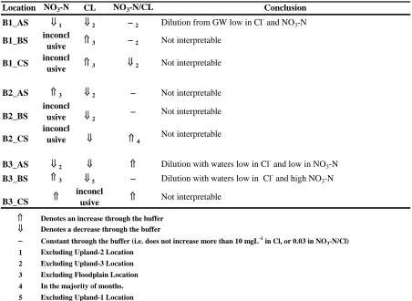
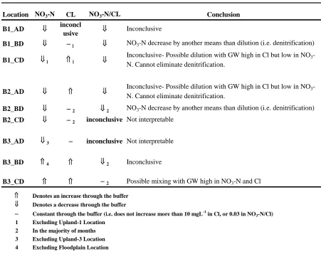
Nitrate/Chloride Ratios ... 83

Soils... 86

Soil Classification ... 86

Particle Size Analysis ... 87

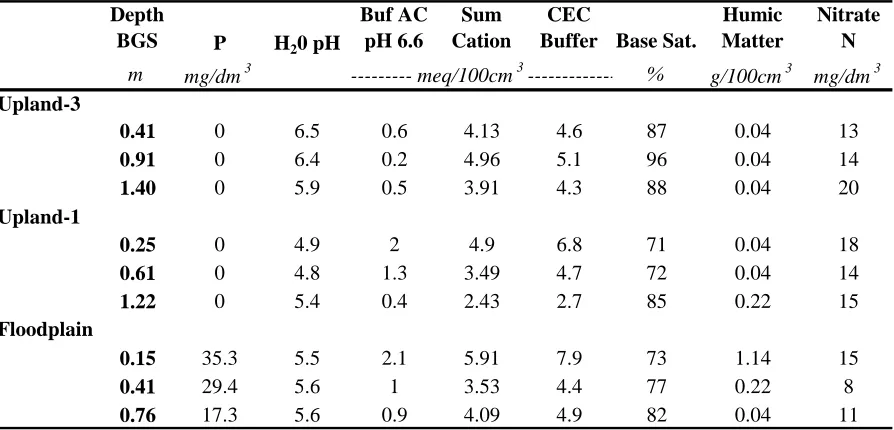
Chemical Analysis ... 87

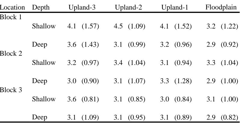
Total Organic Carbon and Dissolved Organic Carbon ... 89

Redox Potential ... 90

Redox Potential, Water Table Elevation and Nitrate-N Comparison ... 91

Nitrate Correlations with Other Groundwater Constituents ... 92

CONCLUSIONS... 94

REFERENCES ... 114

CHAPTER 4. CONCLUSIONS ... 118

APPENDICES ... 122

CHAPTER 2 APPENDICES ... 123

APPENDIX A. Hydraulic Gradient and Flow Direction ... 124

APPENDIX B. TOC, NH3-N, and Cl ... 125

APPENDIX C. Soil Profile Textures ... 131

(9)

vi

APPENDIX E. Reduction Oxidation Potential and Water Table Comparison Over Time

... 140

APPENDIX F. Seasonal Trends in Reduction Oxidation Potential ... 148

APPENDIX G. Groundwater Velocity Tables ... 152

CHAPTER 3 APPENDICIES ... 154

APPENDIX A. NO3--N concentration trends for each depth in each block and location ... 155

APPENDIX B. Seasonal Block NO3--N concentration means ... 161

APPENDIX C. ... 164

NO3--N, Cl and NO3-N/Cl Data for Blocks ... 164

APPENDIX D. NO3--N, Cl and NO3-N/Cl Data for Individual Transects Within Blocks ... 173

APPENDIX E. Soils ... 200

APPENDIX F. USDA Soil Classification at Water Quality Depths ... 204

APPENDIX G. NCDA & CS Soil Analysis ... 208

APPENDIX H. TOC and DOC Concentration Analysis ... 209

APPENDIX I. TOC, NH3-N, and Cl... 211

APPENDIX J. Additional redox potential and water table elevation and NO3--N comparison ... 217

APPENDIX K. Multivariate Groundwater Constituent Correlation Matrices ... 222

(10)

vii

LIST OF TABLES

CHAPTER 2.

Table 1. Water quality well locations in the buffer and distances from the stream ... 28

Table 2. Mean TOC concentrations (mg L-1)... 44

Table 3. Ground surface slope along surveyed transects in Block 1, 2 and 3 ... 44

Table 4. Percentage of days that the water table was within 0.5 m of the soil surface ... 45

Table 5. Travel time from cropped field edge to stream (125 m) for differing soil types and low, mid, and high hydraulic gradients ... 46

CHAPTER 3. Table 1. Water quality well locations in the buffer and distances from the stream ... 75

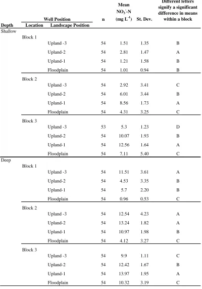
Table 2. Mean NO3--N concentrations ... 98

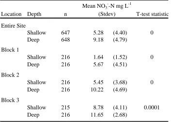
Table 3. Results of t-test to compare shallow and deep well depth mean NO3--N concentrations ... 99

Table 4. Summary of mean NO3--N concentrations and overall mean percent difference for shallow and deep depths ... 99

Table 5. Upwelling scenarios based on NO3--N and Cl concentrations and the NO3-N/Cl ratio ... 100

Table 6. Upwelling conclusions based on NO3--N and Cl concentration, and NO3-N/Cl ratio for shallow and deep wells for all blocks ... 100

Table 7. Dilution conclusions based on NO3--N and Cl concentration, and NO3-N/Cl ratio for individual shallow well transects ... 101

Table 8. Dilution conclusions based on NO3--N and Cl concentration, and NO3-N/Cl ratio for individual deep well transects ... 102

Table 9. NCDA & CS Block 1 soil analysis results ... 103

Table 12. Mean TOC concentrations (mg L-1)... 104

Table 13. Site Shallow groundwater constituent multivariate correlations ... 105

Table 14. Site Deep groundwater constituent multivariate correlations ... 105

APPENDICES ... 122

Table C. 1. Block 1 Transect A, Upland-3 Position ... 131

(11)

viii

Table C. 4. Block 1 Transect C, Upland-1 Position... 132

Table G.1. Estimated Darcy and linear velocity at the depth of sampling wells and time to reach stream along groundwater flow paths from Field Edge for different estimations of saturated hydraulic conductivity of soils for a hydraulic gradient 0.000775 (m/m) ... 152

Table F.1. USDA Soil Classification at the Shallow well depth for different locations . 204 Table F.2. USDA Soil Classification at the deep well depth for different locations ... 206

Table G.1. NCDA & CS chemical analysis for all locations sampled ... 208

Table H.1. Shallow depth TOC and DOC concentrations ... 209

Table H.2. Deep depth TOC and DOC concentrations ... 210

Table J.1. High water table data table for the shallow and deep depth wells in Block 1 transect B ... 218

Table J.2. Low water table data table for the shallow and deep depth wells in Block 1 transect B ... 219

Table J.3. High water table data table for the shallow and deep depth wells in Group 2 transect B ... 219

Table J.4. Low water table data table for the shallow and deep depth wells in Block 2 transect B ... 220

Table J.5. High water table data table for the shallow and deep depth wells in Block 3 transect B ... 220

(12)

ix

LIST OF FIGURES

CHAPTER 1. 1

Figure 1. Schematic of the USDA Riparian Forested Buffer Zones (USDA-NRCS, 1997) 5 CHAPTER 2. 12

Figure 1. Schematic of the USDA Riparian Forested Buffer Zones (USDA-NRCS, 1997.

... 22

Figure 2. Land cover of riparian buffer study site ... 22

Figure 3. NRCS soil survey of CDS Farms site... 24

Figure 4. General soil profile of the upland site ... 24

Figure 5. Study site instrumentation ... 30

Figure 6. Redox probe before and after installation ... 31

Figure 7. Recorded and normal monthly rainfall ... 47

Figure 8. Daily rainfall at the study site from January 1, 2006 to July 31, 2007 ... 47

Figure 9. Land surface contours for study site ... 48

Figure 10. Land surface contours with cross section transect locations ... 49

Figure 11. Cross section of Block 1 transect ... 50

Figure 12. Cross section of Block 2 transect ... 50

Figure 13. Cross Section of Block 3 transect ... 51

Figure 14. Cross section of Blocks 1, 2, and 3 transects in reference to the stream ... 51

Figure 15. Stream channel profile along Blocks 1, 2 and 3 ... 52

Figure 16. Block 1 local water table with ground surface at 0 m at specified distances from the stream during the study period with daily rainfall ... 53

Figure 19. Block 1 local water table depth and angle of groundwater flow direction. ... 54

Figure 20. Groundwater flow direction at different times during the study period ... 55

Figure 21. Block 1 local water table depth and hydraulic gradient over time. ... 56

Figure 22. Site redox averages for shallow depth. ... 57

(13)

x

Figure 24. 2006 low water table conditions 8/31/06, a) Block 1, b) Block 2, c) Block 3 . 58 Figure 25. 2007 low water table conditions 7/15/07, a) Block 1, b) Block 2, c) Block 3 . 59 CHAPTER 3. 63

Figure 1. Land cover of riparian buffer study site ... 71

Figure 2. NRCS soil survey of CDS Farms site with the riparian area studied outlined in red ... 72

Figure 3. General soil profile of the upland area ... 73

Figure 4. Study site instrumentation. ... 74

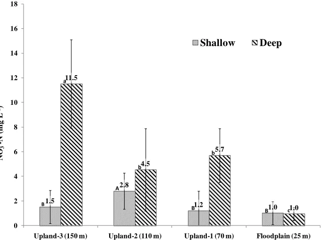
Figure 5. Overall site NO3--N average concentration for different locations and distances from the stream. ... 106

Figure 6. Block 1 NO3--N average concentration for different distances from the stream. ... 106

Figure 7. Block 2 average NO3--N concentration for different distances from the stream. ... 107

Figure 8. Block 3 NO3--N average concentration for different distances from the stream. ... 107

Figure 9. Average NO3--N concentration for different locations by block across the site in shallow wells. n=54 for except Field, Block 3 where n=53. Significant differences are shown by letters within buffer locations. ... 108

Figure 10. Average NO3--N concentration for different locations by block across the site in deep wells ... 108

Figure 11. Site shallow seasonal mean NO3--N concentrations for locations within the buffer. Winter n=45, Spring n=54 Summer n=36, Fall n=27. Significant differences are shown by letters within buffer locations. ... 109

Figure 12. Site deep seasonal mean NO3--N concentrations for locations within the buffer. ... 109

Figure 13. Block 1 Deep NO3--N concentration averages ... 110

Figure 14. Block 1 Deep Cl concentration averages ... 110

Figure 15. Block 1 Deep NO3--N/Cl ratios ... 111

Figure 16. Soil sample locations analyzed by NCDA & CS ... 112

Figure 17. Shallow depth redox potential means with threshold range marked. ... 113

Figure 18. Deep depth redox potential means with threshold range marked. ... 113

APPENDICES ... 122

(14)

xi

Figure B.2. Block 1 TOC means ... 125

Figure B.5. Overall NH3-N means ... 127

Figure B.6. Block 1 NH3-N means ... 127

Figure B.9. Overall Cl means ... 129

Figure B.10. Block 1 Cl means ... 129

Figure D.1. Block 1 water table elevations at specified distances from the stream ... 134

Figure D.2. Block 2 water table elevation at specified distances from the stream ... 134

Figure D.3. Block 3 water table elevation at specified distances from the stream ... 135

Figure D.4. Upland-3 location water table elevation for Blocks 1, 2 and 3 ... 135

Figure D.5. Upland-3 location local water table below ground surface for Blocks 1, 2, and 3... 136

Figure D.6. Upland-2 location water table elevation for Blocks 1, 2 and 3 ... 136

Figure D.8. Upland-1 location water table elevation for Blocks 1, 2 and ... 137

Figure D.10. Floodplain location water table elevation for Blocks 1, 2 and 3 ... 138

Figure D.11. Floodplain local water table below ground surface for Blocks 1, 2, and 3 139 Figure E.1. Redox averages for Block 1 by location and depth ... 140

Figure E.2. Block 1 shallow redox trends for different distances from the stream channel ... 140

Figure E.3. Block 1 deep redox trends for different distances from the stream channel . 141 Figure E.4. Redox averages for Block 2 by location and depth ... 141

Figure E.5. Block 2 shallow redox trends for different distances from the stream channel ... 142

(15)

xii

Figure E.8. Block 3 shallow redox trends for different distances from the stream channel

... 143

Figure E.9. Block 3 deep redox trends for different distances from the stream channel . 144 Figure F.1. Site redox seasonal averages for shallow depth by location ... 148

Figure F.2. Site redox seasonal averages for deep depth by location ... 148

Figure F.3. Block 1 redox seasonal averages for shallow by location ... 149

Figure F.4. Block 1 redox seasonal averages for deep by location ... 149

Figure A.1. Block 1 NO3--N average concentration over time in shallow wells ... 157

Figure A.2. Block 1 NO3--N average concentration over time in deep wells where distance is represented by distance from the stream ... 158

Figure A.4. Block 2 NO3--N average concentration over time in deep wells. ... 159

Figure A.6. Block 3 NO3--N average concentration over time in deep wells ... 160

Figure B.1. Seasonal variations in average NO3--N concentration for the shallow depth in Block 1 based on well location. ... 161

Figure B.2. Seasonal variations in average NO3--N concentration for the deep depth in Block 1 based on well location. ... 161

Figure B.3. Seasonal variations in average NO3--N concentration for the shallow wells in Block 2 based on well location. ... 162

Figure B.4. Seasonal variations in average NO3--N concentration for the deep wells in Block 2 based on well location. ... 162

Figure B.5. Seasonal variations in average NO3--N concentration for the shallow wells in Block 3 based on well location. ... 163

Figure B.6. Seasonal variations in average NO3--N concentration for the deep wells in Block 3 based on well location ... 163

Figure C.1. Block 1 Shallow NO3--N concentration averages ... 164

Figure C.2. Block 1 Shallow Cl concentration averages ... 164

(16)

xiii

Figure C.4. Block 1 Deep NO3--N concentration averages ... 165

Figure C.5. Block 1 Deep Cl concentration averages ... 166

Figure C.6. Block 1 Deep NO3--N/Cl ratios ... 166

Figure C.9. Block 2 Shallow NO3--N/Cl ratios ... 168

Figure C.15. Block 3 Shallow NO3--N/Cl ratios ... 171

Figure D.1. Block 1 Transect A Shallow NO3-N... 173

Figure D.2. Block 1 Transect A Shallow Cl ... 173

Figure D.3. Block 1 Transect A Shallow NO3-N/Cl ... 174

Figure D.4. Block 1 Transect A Deep NO3-N ... 174

Figure D.5. Block 1 Transect A Deep Cl ... 175

Figure D.6. Block 1 Transect A Deep NO3-N/Cl ... 175

Figure D.7. Block 1 Transect B Shallow NO3-N ... 176

Figure D.8. Block 1 Transect B Shallow Cl ... 176

Figure D.9. Block 1 Transect B Shallow NO3-N/Cl ... 177

Figure D.10. Block 1 Transect B Deep NO3-N ... 177

Figure D.11. Block 1 Transect B Deep Cl ... 178

Figure D.12. Block 1 Transect B Deep NO3-N/Cl... 178

Figure D.13. Block 1 Transect C Shallow NO3-N ... 179

Figure D.14. Block 1 Transect C Shallow Cl ... 179

Figure D.15. Block 1 Transect C Shallow NO3-N/Cl ... 180

Figure D.16. Block 1 Transect C Deep NO3-N ... 180

(17)

xiv

Figure D.18. Block 1 Transect C Deep NO3-N/Cl... 181

Figure D.31. Block 2 Transect C Shallow NO3-N ... 188

Figure D.35. Block 2 Transect C Deep Cl ... 190

(18)

xv

Figure D.53. Block 3 Transect C Deep Cl ... 199

Figure I.1. Overall site TOC means with error bars indicating  one standard deviation 211 Figure I.2. Block 1 TOC means with error bars indicating  one standard deviation ... 211

Figure I.3. Block 2 TOC means with error bars indicating  one standard deviation ... 212

Figure I.4. Block 3 TOC means with error bars indicating  one standard deviation ... 212

Figure I.5. Overall NH3-N means with error bars indicating  one standard deviation .. 213

Figure I.6. Block 1 NH3-N means ... 213

Figure I.7. Block 2 NH3-N means with error bars indicating  one standard deviation .. 214

Figure I.8. Block 3NH3-N means with error bars indicating  one standard deviation ... 214

Figure I.9. Overall Cl means with error bars indicating  one standard deviation ... 215

Figure I.10. Block 1 Cl means with error bars indicating  one standard deviation ... 215

Figure K.1. Site shallow matrix for groundwater constituent correlation ... 222

Figure K.2. Site deep matrix for groundwater constituent correlation ... 223

Figure K.3. Site Upland-3 shallow location groundwater constituent multivariate correlations and matrix ... 224

Figure K.4. Site Upland-3 deep location groundwater constituent multivariate correlations and matrix ... 225

Figure K.6. Upland-2 deep location groundwater constituent multivariate correlations and matrix ... 227

Figure K.8. Site Upland-1 deep location groundwater constituent multivariate correlations and matrix ... 229

(19)

xvi

Figure K.10. Site Floodplain deep location groundwater constituent multivariate

correlations and matrix ... 231 Figure K.11. Block 1 shallow groundwater constituent multivariate correlations and matrix ... 232 Figure K.12. Block 1 deep groundwater constituent multivariate correlations and matrix ... 233 Figure K.13. Block 2 shallow groundwater constituent multivariate correlations and matrix ... 234 Figure K.14. Block 2 deep groundwater constituent multivariate correlations and matrix ... 235 Figure K.15. Block 3 shallow groundwater constituent multivariate correlations and matrix ... 236 Figure K.16. Block 3 deep groundwater constituent multivariate correlations and matrix ... 237 Figure K.17. Block 1 Upland-3 shallow groundwater constituent multivariate correlations and matrix ... 238 Figure K.18. Block 1 Upland-3 deep groundwater constituent multivariate correlations and matrix ... 239 Figure K.19. Block 1 Upland-2 shallow groundwater constituent multivariate correlations and matrix ... 240 Figure K.20. Block 1 Upland-2 deep groundwater constituent multivariate correlations and matrix ... 241 Figure K.21. Block 1 Upland-1 shallow groundwater constituent multivariate correlations and matrix ... 242 Figure K.22. Block 1 Upland-1 deep groundwater constituent multivariate correlations and matrix ... 243 Figure K.23. Block 1 Floodplain shallow groundwater constituent multivariate

(20)

xvii

Figure K.28. Block 2 Upland-2 deep groundwater constituent multivariate correlations and matrix ... 249 Figure K.29. Block 2 Upland-1 shallow groundwater constituent multivariate correlations and matrix ... 250 Figure K.30. Block 2 Upland-1 deep groundwater constituent multivariate correlations and matrix ... 251 Figure K.31. Block 2 Floodplain shallow groundwater constituent multivariate

correlations and matrix ... 252 Figure K.32. Block 2 Floodplain deep groundwater constituent multivariate correlations and matrix ... 253 Figure K.33. Block 3 Upland-3 shallow groundwater constituent multivariate correlations and matrix ... 254 Figure K.34. Block 3 Upland-3 deep groundwater constituent multivariate correlations and matrix ... 255 Figure K.35. Block 3 Upland-2 shallow groundwater constituent multivariate correlations and matrix ... 256 Figure K.36. Block 3 Upland-2 deep groundwater constituent multivariate correlations and matrix ... 257 Figure K.37. Block 3 Upland-1 shallow groundwater constituent multivariate correlations and matrix ... 258 Figure K.38. Block 3 Upland-1 deep groundwater constituent multivariate correlations and matrix ... 259 Figure K.39. Block 3 Floodplain shallow groundwater constituent multivariate

(21)

1

CHAPTER 1. GENERAL INTRODUCTION Historical Background

Non-point source (NPS) pollution has negatively impacted streams and rivers across the United States. North Carolina’s water resources including, the Neuse and Tar-Pamlico river basins, have been impacted by nonpoint source pollution. Water quality has been a concern in North Carolina for over 100 years. Legislation was passed in 1887 to eliminate the throwing of dead stock into the Neuse River and its tributaries (NCDWQ, 2007). Water quality management strategies in North Carolina have come a long way since 1887. More recently, sediment load and nutrient enrichment of streams and rivers in the North Carolina Coastal Plain have become the primary cause of many surface water quality concerns and problems (Duda, 1982; Spruill, 2004).

In 1988, the Neuse River basin was declared as ―nutrient sensitive waters‖ and a nutrient management plan was developed to control the occurrence of fish kills and to reduce point and NPS pollution to improve stream health. Also during the 1980s, the Tar-Pamlico River basin experienced an increasing number of fish kills and declining stream health that was attributed to excess nutrient loading. As a result, in 1989, the Environmental

(22)

2

achieve nutrient reduction goals throughout the basin. Initially, the nonpoint source component of Phase II was voluntary, but after two years it was found that more stringent rules were necessary to achieve the desired water quality benefits in the basin. The new rules adopted regulations associated with riparian buffers, nutrient management, stormwater, and agriculture. Phase III (2005-2014) continued the strategy that was established during Phase II and extended the 30% nitrogen reduction goal from baseline conditions established when the nutrient strategy was first implemented in 1991. Reducing nitrogen inputs into

watercourses continues to be a common goal in the two river basins mentioned here as well as other watersheds across the state.

Nitrate-nitrogen (NO3--N), a constituent of NPS pollution, is a form of nitrogen that

contributes nitrogen loadings to watercourses. Excessive NO3--N concentrations that reach

(23)

3

applicants to mitigate for protected activities and the delegation rule allows local governments to implement buffer rules within their jurisdictions (NCDWQ, 2002).

Conservation Reserve Enhancement Program

The Conservation Reserve Enhancement Program (NC CREP) was established to promote best management practices (BMPs) to improve water quality in impaired

watersheds. NC CREP is a combined effort between the North Carolina Division of Soil and Water Conservation, NC Clean Water Management Trust Fund, the Ecosystem Enhancement Program (EEP), and the Farm Service Agency – United States Department of Agriculture (USDA) (NC CREP, 2006). These agencies work together under NC CREP to resolve water quality issues in the Neuse, Tar-Pamlico, Chowan river basins and the Jordan Lake

(24)

4 Riparian Buffers

Riparian buffers are the primary BMP promoted by NC CREP. Riparian buffers are strips of land which are managed for the improvement of water quality by controlling NPS pollution and protecting the stream environment and habitat (Lowrance et al., 1997). Researchers have shown that riparian buffers improve water quality and reduce the amount of NO3--N transported into receiving watercourses (Peterjohn and Correll, 1984; Gilliam,

1994; Gilliam et al., 1997; Lowrance, 1997; Dukes, 2002; Spruill, 2004). Riparian buffers also act as sinks for other nutrients, herbicides and sediments that can potentially pollute streams and rivers (Lowrance et al., 1984; Vellidis and Lowrance, 2004).

Riparian buffers can improve the quality of both older, deeper groundwater that is discharging from longer flow paths as well as younger groundwater, which generally takes a more shallow flow path (Puckett and Hughes, 2005). Above ground, the riparian buffer acts as a sediment filter for surface runoff. Vegetation on stream banks contributes to leafy debris on the streambed and surrounding areas while providing bank stability. Leafy debris

contributes to the amount of organic material below the streambed and provides conditions favorable for the denitrification of deeper groundwater (Spruill, 2000).

(25)

5

because of wetter soil conditions. Upslope from Zone 1 is Zone 2 which is a managed forest that can be periodically harvested to remove pollutants taken up through vegetation. Zone 2 is designed to remove pollutants in subsurface flow and surface runoff by the processes of biological and chemical transformation in the subsurface as well as through storage in woody vegetation, infiltration, and sediment deposition in surface grasses and shrubs. Trees planted in this area can be selectively harvested according to a forestry management plan, provided the zone is replanted with seedlings to continue the process of pollutant removal. Upslope of Zone 2 is Zone 3, which consists of a grass filter strip whose function is to slow and disperse concentrated surface flow into sheet flow to remove sediment and associated pollutants (Vellidis and Lowrance, 2004). These three zones work together to decrease the amount of nitrogen and other harmful nutrients, sediments and herbicides from upslope sources from reaching and contaminating surface waters.

(26)

6 Riparian Buffer Processes for Pollutant Reduction

Pollutant removal within riparian buffers can be divided into two categories, surface removal and subsurface removal. Pollutants that are removed on the surface of the riparian buffer are sediments and nutrients such as phosphorus. They are most effectively trapped by grasses, brush and shrubs that are located in Zone 3. Subsurface pollutants such as NO3--N,

can be transformed to a less harmful form of nitrogen gas, by the microbial mediated process of denitrification (Madigan et. al, 2000). Another occurrence that can lead to an apparent decrease of groundwater NO3--N concentration in the subsurface is dilution. Dilution occurs

by deeper groundwater that is less NO3--N rich, discharging close to the stream. It mixes

with shallow groundwater, reducing the concentration near the stream, although the total loading to the receiving water body is the same (Altman and Parizek, 1995).

There are several factors that influence the denitrification effectiveness of riparian buffers. Organic carbon, the presence of denitrifying microbes, anaerobic soil conditions as influenced by the water table and the hydrologic flow path of groundwater are all necessities for this process to occur and successfully reduce NO3--N (Knowles, 1982; Korom, 1992;

Puckett, 2004). The water table and hydrologic flow path may vary between buffers and fluctuate seasonally within a single riparian buffer and thus can affect denitrification rate. The position of the water table depends on soil properties, landscape position, upslope area and precipitation. During drought conditions, the water table may not transport NO3--N rich

(27)

7 Hydrology and Buffer Effectiveness

Some researchers have reported buffer effectiveness of 90 to 100% reduction in NO3-

-N concentrations (Lowrance, 1992; Lee et al., 2000). However, such high reductions in -NO3

--N are not always observed in buffers. It is shown in the literature that some buffers are more suited to attenuate nitrogen (Osmond, 2002). Mayer (2007) found that among 89 individual riparian buffer studies, wider buffers were more effective at removing nitrogen. However, he cautions that there are other factors besides buffer width that determine effectiveness such as vegetation depth and hydrological flow paths.

Several studies have shown that the hydrology beneath a riparian buffer is a major component of buffer success and thus should be considered (Hill, 1996; Puckett, 2004; Angier et al., 2005; Mayer et al., 2007). Among 13 sites across the United States, Puckett (2004) cited other means by which the hydrology can affect the apparent decrease or increase of NO3--N including: long residence times (> 50 years along groundwater flow paths),

dilution of NO3--N enriched groundwater with older depleted groundwater, bypassing of

riparian zones because of drains or ditches, and movement of groundwater along deep flow paths below reducing zones (Puckett, 2004). According to Hill (1996) any condition that allows NO3--N enriched groundwater to bypass reducing zones of the buffer limits the

denitrification capacity. Therefore, hydrology is a critical element of buffer success and can be considered a tool in the prediction and evaluation of NO3--N loss in a riparian zone

(Mayer et al., 2007).

(28)

8

performing buffer. It has been shown that some buffers attenuate pollutants at higher rates than others, but the reasons are unclear. Hydrology clearly plays a major role in determining buffer NO3--N reduction effectiveness.

The purpose of this study is to evaluate a NC CREP riparian buffer with respect to NO3--N concentration removal and determine a correlation between the efficiency of NO3--N

removal and the hydrology found on the site in order to help guide future NC CREP enrollments. Prior research has shown that just because a riparian buffer exists does not necessarily imply that it is achieving water quality goals. Therefore, enrolling wide widths of land into this conservation program based solely on proximity to streams may not maximize water quality benefits that justify the expense of land acquisition.

Objectives

The site for this study was enrolled in NC CREP in 2003 and was initially chosen based on relative age of the buffer, landscape position, slope, the absence of tile drains, ditches and gullies that would short-circuit surface and groundwater to the stream in accordance with NC CREP (2006). The site was chosen to investigate the water quality benefits of newly established enrollments that under current criteria qualified as a buffer, even though it was upslope of a much older existing hardwood forested swamp.

The objectives of this research were to:

1. Evaluate NO3--N reduction effectiveness of a riparian buffer enrolled in NC CREP in

the upper coastal plain of North Carolina.

2. Evaluate the hydrology beneath the study site and its effect on NO3--N trends.

(29)

9

REFERENCES

Altman, S.J., and R.R. Parizek. 1995. Dilution of Nonpoint-Source Nitrate in Groundwater. J. Environ. Qual. 24:707-718.

Angier, J.T., G.W. McCarty, K.L. Prestegaard. 2005. Hydrology of a first-order riparian zone and stream, mid-Atlantic coastal plain, Maryland. Journal of Hydrology. 309 (2005): 149-166.

Duda, A.M.1982. Municipal Point Source and Agricultural Nonpoint Source Contributions to Coastal Eutrophication. Water Resources Bulletin. 18(3): 397-407.

Dukes, M.D., R.O. Evans, J.W. Gilliam, S.H. Kunickis. 2002. Effect of riparian buffer width and vegetation type on shallow groundwater quality in the middle coastal plain of North Carolina. Trans. ASAE. 45(2): 327-336.

Gilliam, J.W. 1994. Riparian Wetlands and Water Quality. J. Environ. Qual. 23: 896-900. Gilliam, J.W., D.L. Osmond, R.O. Evans. 1997. Selected Agricultural Best Management

Practices to Control Nitrogen in the Neuse River Basin. North Carolina Agricultural Research Service Technical Bulletin 311, North Carolina State University, Raleigh, NC.

Hill, A.R. 1996. Nitrate Removal in Stream Riparian Zones. J. Environ. Qual. 25: 743-755. Knowles, R. 1982. Denitrification. Microbiological Reviews. 46(1): 43-70.

Korom, S. F. 1992. Natural Denitrification in the Saturated Zone: A Review. Water Resources Research. 28(6): 1657-1668.

Lee, K.H., T.M. Isenhart, R.C. Schultz, S.K. Mickelson. 2002. Multispecies Riparian Buffers Trap Sediment and Nutrients during Rainfall Simulations. J. Environ. Qual. 29: 1200-1205.

Lowrance, R., R. Todd, J. Fail, O. Hendrickson, R. Leonard, L. Asmussen. 1984. Riparian Forests as Nutrient Filters in Agricultural Watersheds. Bioscience. 34(6): 374-377. Lowrance, R.R. 1992. Groundwater Nitrate and Denitrification in a Coastal Plain Riparian

(30)

10

Lowrance, R., L. S. Altier, J. D. Newbold, R. R. Schanabel, P. M. Groffman, J. M. Denver, D. L. Correll, J. W. Gilliam, J. R. Robinson, R. B. Brinsfield, K. W. Staver, W. Lucas, A. H. Todd. 1997. Water quality functions of riparian forest buffers in Chesapeake Bay watersheds. Environmental Management. 21(5): 687-712.

Madigan, M.T., J.M. Martinko, J. Parker. 2000. Biology of Microorganisms. Upper Saddle River, N.J.: Prentice-Hall, Inc.

Mayer, P.M., S.K. Reynolds, Jr., M.D. McCutchen, T.J. Canfield. 2007. Meta-Analysis of Nitrogen Removal in Riparian Buffers. J. Environ. Qual. 36:1172-1180.

NC CREP. 2006. NC CREP Water Quality Minimum Criteria. Washington, NC: North Carolina Conservation Reserve Enhancement Program. Available at:

http://www.enr.state.nc.us/dswc/pages/NC CREP.html. Accessed 29 November 2007. NCDWQ. 2002. Nonpoint Source Management Program: Tar-Pamlico Nutrient Strategy.

Raleigh, NC: North Carolina Division of Water Quality. Available at: http://h2o.enr.state.nc.us/nps/tarpam.htm. Accessed 25 May 2007.

NCDWQ. 2007. Nonpoint Source Management Program. Raleigh, NC: North Carolina Division of Water Quality. Available at: http://h2o.enr.state.nc.us/nps. Accessed 26 November 2007.

NRC. 2002. Riparian Areas: Functions and Strategies for Management. Washington, D.C.: National Academy Press.

Osmond, D.L., J.W. Gilliam and R.O. Evans. 2002. Riparian Buffers and Controlled Drainage to Reduce Agricultural Nonpoint Source Pollution, North Carolina Agricultural Research Service Technical bulletin 318, North Carolina State University, Raleigh, NC.

Peterjohn, W.T., and D.L. Correll. 1984. Nutrient dynamics in an agricultural watershed: observations on the role of a riparian forest. Ecology. 65(5): 1466-1475.

Puckett, L.J. 2004. Hydrogeologic controls on the transport and fate of nitrate in groundwater beneath riparian buffer zones: results from thirteen studies across the United States. Water Science and Technology. 49(3): 47-53.

Puckett, L.J., and B.L. Hughes. 2005. Transport and Fate of Nitrate and Pesticides: Hydrogeology and Riparian Zone Processes. J. Environ. Qual. 34: 2278-2292. Spruill, T. B. 2000. Statistical Evaluation of Effects of Riparian Buffers on Nitrate and

(31)

11

Spruill, T.B. 2004. Effectiveness of riparian buffers in controlling ground-water discharge of nitrate to streams in selected hydrogeologic settings of the North Carolina Coastal Plain. Water Science and Technology. 49(3): 63-70.

USDA-NRCS. 1997. Riparian Forest Buffer Conservation Practice Job Sheet. Washington, D.C.: United States Department of Agriculture-Natural Resources Conservation Service.

(32)

12

CHAPTER 2. HYDROLOGY OF A RIPARIAN BUFFER IN THE UPPER COASTAL PLAIN OF NORTH CAROLINA AND ITS EFFECT ON NITRATE REDUCTION

INTRODUCTION

Recent riparian buffer studies have placed emphasis on subsurface hydrology and its importance in achieving NO3--N reduction (Hill, 1996; Vidon and Hill, 2004b; Mayer, 2007).

In agricultural watersheds, nitrogen enters groundwater through the application of fertilizer and animal waste. Inorganic and organic nitrogen in fertilizers applied to cropland are

generally not completely used by plants or microorganisms. Residual nitrate (NO3--N), either

from direct application or from various transformations by aerobic soil microorganisms (e.g. mineralization, ammonification, and nitrification) is generally the nitrogen species of most concern for water quality. Groundwater is the pathway by which NO3--N moves beneath the

soil surface and enter streams, rivers, lakes, and ponds. Following precipitation, soluble NO3--N leaches and moves through the soil water system to groundwater. Excess NO3--N in

waterways causes eutrophication, resulting in low dissolved oxygen and death of aquatic life (Martin et al., 1999).

Denitrification is the primary pathway soil NO3--N is transformed under anaerobic

conditions and returned to the atmosphere as nitrogen gas (Sylvia et al., 1998). Denitrification is the process by which the majority of NO3--N in groundwater can be

transformed. There are several requirements for denitrification to occur: (1) denitrifying microorganisms, (2) organic carbon, (3) anaerobic soil conditions and (4) a supply NO3--N.

(33)

13

denitrification capacity of a riparian buffer. As the water table rises and O2 availability

decreases, facultative and obligate anaerobes begin to use NO3--N as an electron acceptor

instead of O2 (Knowles, 1982; Korom, 1992). As long as soil pores remain anaerobic and a

source of carbon is available, NO3--N will be denitrified until the NO3--N substrate limits

denitrification. After NO3--N is depleted other compounds will serve as electron acceptors

such as manganese (IV), ferric iron (III), and sulfate (SO42-) (Korom, 1992).

An increased residence time allows groundwater NO3--N more contact with reducing

environments. A longer residence time provides more opportunity for denitrification, especially if other factors such as organic carbon are limiting. Therefore, the hydrology beneath a riparian buffer must be understood to explain and predict the fate of NO3--N in the

buffer.

Researchers have found that NO3--N removal in riparian buffers is variable, (Maitre et

al., 2005) and is not always a function of buffer width (Mayer et al., 2007; Vidon and Hill, 2004b). Many researchers attribute the effectiveness of buffers to hydrologic factors (Hill, 1996; Osmond, 2002; Puckett, 2004). These factors include: residence times along groundwater flow paths, dilution of NO3--N rich waters by less concentrated older

groundwater, the bypassing of riparian zones by tile drains or ditches, and the movement of groundwater along deep flow paths below shallower, organic rich reducing zones (Puckett, 2004). Hill (1996), states that riparian zones that effectively remove NO3--N have

(34)

14

the riparian area. In this setting, groundwater travels at shallow depths and is in contact with organic carbon in the root zone, increasing the potential for NO3--N removal and

denitrification.

Vidon and Hill (2004b, c) studied different landscape hydrogeologic characteristics that influence the hydrology of riparian sites and the efficiency in reducing NO3--N

concentration in the buffer. Their study included 8 stream riparian sites in southern Ontario, Canada. They concluded that a concave riparian profile favored interactions between subsurface water and surface soil horizons, and were more conducive to denitrification and plant uptake. Conversely a convex riparian profile or topography favored water tables further from the surface and deeper subsurface flow paths where denitrification and plant uptake was less likely to occur. In natural riparian areas and riparian wetlands, concave profiles are common, while a convex profile is more indicative of upland topography.

Gold et al. (2001) in their study in Rhode Island concluded that groundwater flow paths and travel time through riparian zones is crucial to buffers reducing NO3--N.

Groundwater flow paths that remain shallow and are underlain by a shallow impermeable layer allows more interaction with plant roots and organic matter. Sites with shallow groundwater flows have been shown in past studies to transform NO3--N more effectively

than sites with deeper groundwater flow paths (Bohlke and Denver, 1995; Simmons et al., 1992; Spruill, 2000; Puckett, 2004). Spruill (2000, 2004) adds that the riparian system can affect older groundwater as well as young groundwater flow paths of older, deeper

(35)

15

factors affecting groundwater flow paths are hydrogeologic setting and soil characteristics (Vidon and Hill, 2004a,c). Puckett (2004) observed a reduction in NO3--N in deeper

groundwater when the flow paths encountered reducing conditions (i.e. anaerobic pockets, a buried supply of organic carbon, and denitrifying microorganisms).

Groundwater flow paths through buffers are not necessarily constant, as they can be influenced by times of drought or high rainfall. For example, in two of the eight buffer sites studied by Vidon and Hill (2004b) water tables fell below the stream water level which resulted in flow reversals.

Another hydrologic occurrence that has been found to complicate observed NO3--N

concentration reduction is dilution. Shallow groundwater rich in NO3--N can be diluted by

less concentrated deeper groundwater upwelling from deeper flow paths discharging near stream locations. Several studies have cited decreasing NO3--N concentrations as the result

of dilution. Altman and Parizek (1995) concluded that it was difficult to confirm NO3--N

removal because dilution was dominating the system. They used the chloride ion (Cl-) concentration to serve as a conservative tracer to determine if dilution was the cause of NO3-

-N concentration reduction. The authors concluded that the total nitrogen loading was not reduced before discharging into the stream (Altman and Parizek, 1995). In another study, Clausen et al. (2000) observed a decrease of 46% in the NO3--N to Cl- ratio through the

buffer. A decrease in the NO3--N to Cl- ratio may be caused by: (1) NO3--N concentration

decrease due to a microbial process or plant uptake, (2) Cl- concentration increase, (3) or both could be occurring simultaneously, but NO3--N concentration could decrease more than

(36)

16

conclude that both microbial processes and dilution from deeper groundwater occurred simultaneously beneath the buffer.

Angier et al. (2005) found the hydrology of a first-order stream in a low-relief landscape in Maryland to be dominated by vertical flow rather than the assumed horizontal flow, and iterated that merely buffer width was not a sufficient parameter in estimating the performance of a riparian buffer. Angier et al. (2005) hypothesized that highly active upwelling zones are likely indicative of origin points for first-order streams in low-relief environments. Angier et al. (2005) also states that ―it is the interplay between the hydrology and biogeochemistry that determines the effectiveness of a riparian buffer as a means for remediation”.

The hydrology of a buffer can also vary seasonally, which in turn may affect NO3--N

retention. Winter water tables are generally higher than in other seasons because of higher precipitation and lower evapotranspiration in the southeast United States. In agricultural settings, inputs of nitrogen to buffers vary seasonally depending on which crop is adjacent to the buffer. Burkhart and Kolpin (1993) found that there were no marked variations in NO3-

-N concentrations although some individual wells did display seasonal variation throughout their study. As the water table elevation rises and falls from seasonal differences in the profile, the newly saturated condition encourages the release of soluble carbon in the soil solution which provides a more available and steady release of an energy source for

(37)

17

both dormant and growing seasons, but the mechanism differed depending on season. They observed that during the dormant season the water table rose and exposed the upper portion of the groundwater to more organic rich soil than during the growing season (Simmons et al., 1992).

A rising water table, along with providing an increasing zone for potential

denitrification, can also add a pulse of NO3--N in groundwater. When NH4+ is nitrified to

NO3--N in unsaturated conditions and the soil then becomes saturated, NO3--N residing in

soil pores is captured and available for transport with groundwater to the stream. Bohlke et al. (2007) observed seasonal variations at the stream which were directly correlated with water table elevations. During the summer and fall where low water table elevations were observed, NO3--N concentrations were low as well. However, during winter and spring when

water table elevations were higher, elevated NO3--N concentrations were observed.

According to the authors, these trends were observed because older groundwater less rich in NO3--N discharged to the stream during low water table periods in the summer and fall. As

the water table rose, NO3--N concentrations were higher because more shallow groundwater

was discharged to the stream from an aerobic zone and did not come into contact with reducing environments before stream discharge (Bohlke et al., 2007).

(38)

18

predictive power in making decisions related to whether a site would experience water quality benefits from a buffer in that location.

The North Carolina Conservation Reserve Enhancement Program (NC CREP) is a program that can benefit from more buffer hydrology research. NC CREP is a combined effort between the North Carolina Division of Soil and Water Conservation, NC Clean Water Management Trust Fund, the Ecosystem Enhancement Program (EEP) and the Farm Service Agency - United States Department of Agriculture (FSA-USDA) (NC CREP, 2006). These agencies work together under NC CREP to resolve water quality issues in the Neuse, Tar-Pamlico, Chowan river basins and the Jordan Lake watershed. The program is voluntary, where by previously agricultural land is enrolled into conservation practices along impaired watercourses to improve water quality. As of 2007, 2,214 ha (5,472 acres) were enrolled in permanent easements and 7,672 ha (18,958 acres) were enrolled in 30 year easements (N. Jones, NC CREP Manager, personal communication, 2007). The Conservation Enhancement Program invests a considerable amount of public money to protect water quality, so

understanding which enrollments perform the best will be critical in its success. This research would enable NC CREP to have more descriptive criteria of which to base riparian buffer enrollment decisions.

(39)

19

(40)

20

MATERIALS AND METHODS

Site Description

The study area is located southeast of Enfield, NC in Halifax County. The site is in the Fishing Creek watershed (Hydrologic Unit 03020102) within the Tar Pamlico River basin. This area of North Carolina is largely agricultural and in the Upper Coastal Plain. The study site consists of a newly established young buffer upslope of an existing mature forested buffer and down gradient of an agricultural field. The area comprising the young buffer was most recently in agricultural row crop production and was located in an upland landscape position. Discussions with the landowner indicated that other historical land uses included pasture for beef cattle. One or two small houses may have also been located within the buffer area several decades ago. This 3.5 ha (8.7 acre) area is currently enrolled as a CP22 buffer in NC CREP, a voluntary program that works to establish BMPs on former agricultural land to protect water quality in impaired watersheds.

(41)

21

The young buffer in the upland landscape position was established with loblolly pine (Pinus taeda L.) in 2003. The estimated density of the pine planting was 720 stems/acre and the seedlings were approximately 1.2-1.8 m tall in 2005. In 2007, the trees ranged from 2.4-4 m in height. The hardwood forested swamp included a channelized intermittent (1st order) stream, approximately 0.6 m (2 ft) deep with smaller less defined channels spread over the floodplain area. The channelized intermittent stream was already buffered by the hardwood forested swamp prior to the establishment of the young CP22 buffer.

(42)

22

Figure 1. Schematic of the USDA Riparian Forested Buffer Zones (USDA-NRCS, 1997)

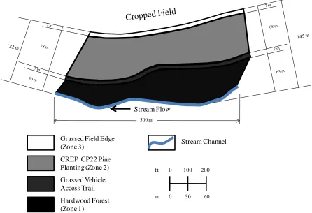
Figure 2. Land cover of riparian buffer study site 300 m

Grassed Field Edge (Zone 3)

CREP CP22 Pine Planting (Zone 2) Grassed Vehicle Access Trail Hardwood Forest (Zone 1)

Stream Channel Stream Flow

ft 0 100 200

(43)

23

(44)

24

Figure 3. NRCS soil survey of CDS Farms site with the riparian area studied outlined in red

Figure 4. General soil profile of the upland site 1 m

2 m

7 m Loamy Sand,

Sandy Loam Sandy Clay Loam,

Clay Loam

Sand, Gravelly Sand

(45)

25 Monitoring

Prior to full site instrumentation groundwater flow direction was determined by using hydraulic head measurements from five wells following the procedure commonly referred to as the Three Point Method (Schwartz, 2003). This was a crucial determination since

groundwater flow determines the path NO3--N takes to the stream. This initial information

was used to install water quality well transects through the buffer as close to parallel with the groundwater flow as possible. During the study period, best-fit hydraulic gradients were determined at different times using hydraulic head data from the water table monitoring wells (Devlin, 2002). This method of determining the hydraulic gradient uses water table

elevations (z), x and y coordinates with matrix solving functions to determine the equation of the water table plane (1),

𝐴𝑥 + 𝐵𝑦 + 𝐶𝑧 − 𝐷 = 0 (1) Where A, B, C and D are coefficients of the water table surface and are used to

calculate the magnitude and direction of the hydraulic gradient (2),

i

=

𝐴2_𝐶+𝐵₂ 2 (2)

(where i is the hydraulic gradient and A, B, and C are coefficients of the water table surface). The direction of flow (3),  is the angle measured from the x-axis.

𝛼 = arctan𝐵_𝐴 (3)

(46)

26

Hydraulic conductivity and groundwater velocities were estimated to determine an approximate groundwater residence time in the buffer. Saturated hydraulic conductivity (Ks)

values were obtained using the results of the particle size analysis and the data of Rawls (1998). Darcy’s equation was used to estimate groundwater velocity through the buffer.

𝑣 = 𝐾_𝑠𝑖 (4) where v = Darcy velocity or the apparent velocity (cm/hr)

Ks = Saturated hydraulic conductivity (cm/hr)

i = hydraulic gradient

Field measurements were attempted to estimate hydraulic conductivity by the Auger Hole Method (vanBeers, 1970), but the water table fell too low in Spring 2007 and never rose to a level where the test could be performed successfully. Instead hydraulic conductivities were obtained from Rawls (1998) who took a database of 953 values of Ks and organized

them based on USDA soil classification.

The hydraulic gradient was calculated using hydraulic head data from 10 wells in a spreadsheet method explained in a previous section, equation (5) is a representation of what the gradient is essentially.

𝑖 =

ℎ1−ℎ2

𝐿 (5)

Where i = hydraulic gradient

h1 and h2 are hydraulic heads (m)

L = Length along flow path (m)

(47)

27

the linear groundwater velocity is a more accurate estimate of groundwater velocity because water flows through the soil pores. In equation (6) vs, the linear groundwater velocity or pore

velocity is calculated.

𝑣

_𝑠

=

𝐾𝑠

𝑛𝑒

𝑖

(6) Where vs = linear groundwater velocity (cm/hr)

Ks = saturated hydraulic conductivity (cm/hr)

ne = effective porosity

i = hydraulic gradient

Therefore, when calculating the velocity of groundwater the linear groundwater velocity will be greater than the Darcy velocity since it factors in the effective porosity of the soil. Both values of velocity are estimates and according to Lamb and Whitman (1969) they can both be used to estimate the time required for water to move through a given distance in soil.

The study site had three replications of monitoring wells that were in three distinct blocks along the intermittent stream. Block 1 was at the most upstream location and Block 3 was the most downstream location.

(48)

28

the hole, backfilled with sand to cover the well screen, and the remainder of the hole was sealed with HOLEPLUG bentonite.

In the upland pine buffer, shallow wells were installed to a depth of 2.1 m (7 ft), screened from 1.5-2.1 m (5-7 ft), and the deep wells were installed to a depth of 3.4 m (11 ft), screened from 2.7-3.4 m (9-11 ft). Wells installed in the existing hardwood forested buffer were placed at the edge of the swamp where flooding was observed to occur more frequently. Because the existing hardwood forested area was a floodplain and at a lower elevation, the nests of wells located there were only installed to a depth of 1.5 m (5 ft) and screened from 0.9-1.5 m (3-5 ft) in the shallow wells. The deep wells in the floodplain were installed to a depth of 2.1 m (7 ft) and screened from 1.5-2.1 m (5-7 ft). The water quality wells in each block were installed based on distance from the agricultural field. The stream running adjacent to the buffer meanders slightly causing there to be a difference in each block’s well distance from the stream (Table 1). A total of 72 water quality wells were installed on the site (3 blocks x 3 transects/block x 4 well nests/transect) (Figure 5).

Table 1. Water quality well locations in the buffer and distances from the stream

Well Location USDA-NRCS Classification

Distance from Stream (m) Upland 3 Zone 3 Interface with Zone 2 150-115

Upland 2 Middle of Zone 2 110-80

Upland 1 Between Zone 1 and Zone 2 70-40

(49)

29

(50)

30

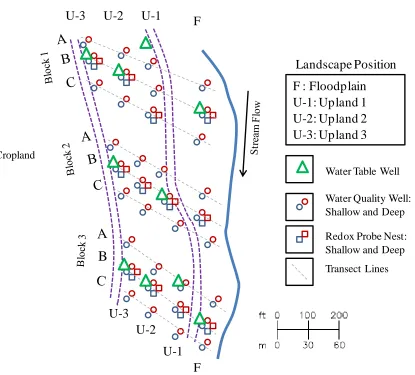
Figure 5. Study site instrumentation

Redox Potential Probes

Platinum tip redox probes were built according to Wafer et al. (2004) and installed in late September and October 2006. Five probes were placed in one 5 cm (2 in) PVC pipe and sealed with a flat end cap. Five holes were drilled in the bottom end cap and one platinum tip electrode was inserted in each hole in order for the platinum tip to have contact with the surrounding soil (Figure 6). The top end cap had a drilled hole for the wires of each probe to

B

Water Table Well

Water Quality Well: Shallow and Deep Redox Probe Nest: Shallow and Deep Transect Lines Cropland

U-3 U-2 U-1 _F

U-3 U-2

U-1 F

F : Floodplain U-1: Upland 1 U-2: Upland 2 U-3: Upland 3

(51)

31

be exposed and was sealed with silicon. A nest of 5 probes each were installed at depths corresponding to the groundwater quality depths in the center transect of each block except for one location in Block 1. This nest would have been in a low area and not representative of the landscape in Block 1 in that location. It was moved downstream from the original location to account for this difference in topography. A total of 120 probes were installed on the site (5 probes/depth x 2 depths/nest x 4 nests/block x 3 blocks).

Figure 6. Redox probe before and after installation

Redox potential (Eh) readings were taken monthly beginning in November 2006 using a Fisher Scientific ® Accumet AP62 Portable pH/mV Meter and a KCl saturated Ag/AgCl reference electrode (Jensen Instruments, Tacoma, WA). Based on soil temperature and pH a correction factor of 204 mV was used to adjust the values of the voltages that would have been measured with a standard hydrogen electrode (Richardson et al., 2001).

Groundwater Sampling

Groundwater quality sampling at the site was performed monthly for 18 months, from January 2006 - July 2007. Sample bottles were pre-acidified with 18 M H2SO4 at the time of

Redox Probe Nest

Water Table Monitoring Well

(52)

32

sampling to halt biological activity. Before sampling, each groundwater well was purged with a submersible pump until dry or when at least three well volumes had been removed. Wells were sampled using a Watermark® bailer that was specific to each well nest to prevent cross well contamination. Samples were put on ice and transported to the NCSU-BAE Environmental Analysis Lab and refrigerated at 4º C until analyzed. Samples were analyzed for total organic carbon (TOC) using the Apollo 9000 (EPA 415.2) in this portion of the study (U.S. EPA, 1983).

Site Survey

A topographic survey of the site was conducted on three occasions. A Topcon Electronic Total Station was used each time. The site was first surveyed in June 2006 where only the young buffer could be surveyed because of dense vegetation in the hardwood forest. In March 2007, the hardwood forest was surveyed and a subsequent survey to verify the previous two surveys was taken in December 2007. Points for ground surface elevation, instrumentation and stream boundaries were collected based on a control point with an assumed elevation of 30.5 m (100 ft) near the cropped field edge. Points collected from the three surveys were examined and imported into AutoCAD® Civil 3D Land Desktop

(53)

33

RESULTS AND DISCUSSION

Rainfall

Rainfall data was collected throughout the study period and is reported in Figure 7 and 8. In Figure 7, the normal monthly rainfall for Enfield, NC (312827) is reported from the State Climate Office of North Carolina and is plotted next to the observed monthly rainfall at the study site. The average yearly rainfall for the study area was approximately 115 cm. In 2006, the study site precipitation was just above normal with 124 cm of rainfall. From January 2007 to July 2007 monthly rainfall totals were less in most months than normal. On average the amount of precipitation received during this period was 68 cm, whereas the site only received 43 cm. Of note, two large storm events occurred during the study period (Figure 8). Tropical storm Alberto and Ernesto caused high rainfall in excess of 90 mm per day and occurred on June 14, 2006 and September 1, 2006 respectively. Another event of note took place in November 2006 where 47 and 59 mm of rain occurred 4 days apart. The floodplain was inundated with water and ponding occurred in upland portions of Block 1 and 2 during these events.

Total Organic Carbon

(54)

34 Topography

The slope of the site was relatively low. Figure 9 shows a contour map of the buffer area. Throughout the site, there was a maximum relative elevation of 30.7 m (100.7 ft) and minimum elevation of 28.9 m (94.7 ft) with an average slope of 1.56%. Within each block, transects were surveyed, graphed and compared (Figure 10-14). Generally speaking, the surveyed transects in each block had low slopes between 1-2%. Block 1 and 2 were similar in slope from the cropped field edge to the stream, 0.98% and 1.09% respectively. Block 3 had the greatest slope of 1.9%. From where the floodplain began in Blocks 1-3, Block 1 had the longest distance from the beginning of the floodplain to the stream channel (23 m) and a slope of 0.95%. Block 2’s floodplain was approximately 13 m wide and had a slope of 0.47%. Block 3’s floodplain was less defined and the steepest among the three blocks (2.15%). The upland areas of Blocks 1 and 2 were more sloped than the floodplain; conversely Block 3 had slopes that were steeper in the region next to the stream than in the upland. Table 3 presents slope data for the site. From the individual transect graphs, (Figures 11-13) convex profiles in upland portions of Blocks 1, 2 and 3 were observed and had concave profiles in the floodplain area of Blocks 1 and 2. Figure 14 shows all three block’s transects relative to stream position.

(55)

35

and Hill (2004b). Therefore, the floodplain was more suited to provide conditions necessary for denitrification than the upland region based on topographical characteristics.

Figure 15 depicts the surveyed stream channel elevation along the buffer. The stream channel elevation decreased 0.16 m (0.5 ft) along the length of the buffer from Block 1 to Block 3 and had an overall slope of 0.05%. After high precipitation events the stream expanded onto the floodplain because of the rising and falling elevation along the channel and shallow depth. This caused the waters to reach up to and at times beyond floodplain monitoring wells.

Soil Profile

Soil profile descriptions were taken at the time of water quality well installations in 2005. The upland planted pine was found to be relatively homogenous in the upper profile with a sandy clay loam, clay loam or sandy loam textures to a depth of approximately 1.8-2 m below ground surface (Figure 4). At all locations in the upland pine area, the upper profile was underlain by sand ranging from coarse to gravely sand below 2 m. At the time of