Fifteenth mathematical and statistical modeling workshop for graduate students

(1)

Fifteenth Mathematical and Statistical Modeling

Workshop for Graduate Students

19 – 29 July 2009

North Carolina State University

Raleigh, NC, USA

Organizers:

Pierre Gremaud, Ilse C.F. Ipsen, Ralph C. Smith

Department of Mathematics

North Carolina State University

This report contains the proceedings of the Industrial Mathematical and

Statistical Modeling Workshop for graduate students, held at the Center

for Research in Scientific Computation at North Carolina State University

(NCSU) in Raleigh, North Carolina, 19 – 29 July 2009.

This was the fifteenth such workshop at NCSU. It brought together 39

graduate students from 33 different universities. The goal of the IMSM

workshop is to expose mathematics and statistics students from around the

country to: real-world problems from industry and government laboratories;

interdisciplinary research involving mathematical, statistical and modeling

components; as well as experience in a team approach to problem solving.

On the morning of the first day, industrial and government scientists

presented six research problems. Each presenter, together with a specially

selected faculty mentor, then guided a team of about 6 students and helped

them to discover a solution. In contrast to neat, well-posed academic

ex-ercises that are typically found in coursework or textbooks, the workshop

problems are challenging real world problems that require the varied

ex-pertise and fresh insights of the group for their formulation, solution and

interpretation. Each group spent the first eight days of the workshop

investi-gating their project and reported their findings in half-hour public seminars

(2)

on the final day of the workshop.

The IMSM workshops have been highly successful for the students as

well as the presenters and faculty mentors. Often projects lead to new

re-search results and publications. The projects can also serve as a catalyst for

future collaborations between project presenter and faculty mentor. More

information can be found at

http://www.ncsu.edu/crsc/events/imsm09/

Statistical and Applied Mathematical Sciences Institute (SAMSI)

CRSC: Center for Research in Scientific Computation (CRSC)

Department of Mathematics, North Carolina State University

Presenters

Erik Gilleland, National Center for Atmospheric Research

John Langstaff, Environmental Protection Agency

Jordan Massad, Sandia National Laboratories

Howard McLeod, UNC Institute for Pharmacogenomics

Frank Meyer, Republic Mortgage Insurance Company

John Peach, MIT Lincoln Laboratory

Faculty mentors

Mansoor Haider, NCSU, Mathematics

Elizabeth Mannshardt-Shamseldin, Duke, Statistics

Alison Motsinger-Reif, NCSU, Statistics

Brian Reich, NCSU, Statistics

Jeff Scroggs, NCSU, Mathematics

Ralph Smith, NCSU, Mathematics

Richard Smith, UNC, Statistics

Student Participants

Aaron Brown, Erin Byrne, Heejun Choi, Lili Ding, Robertas Gabrys, Chad

Griep, Matthew Heaton, Magathi Jayaram, Matthias Katzfuss, Noory Kim,

Jenya Kirshtein, Nitesh Kumar, Busaba Laungrungrong, Yi Li, Michael

Lo-muscio, Mario Morales, Glen Dale Pearson, Kathryn Pedings, Jacob Porter,

William Proctor, Karthik Raghuram, Shahla Ramachandar, Gregory Richards,

(3)

Nishantha Samarakoon, Varada Sarovar, Maryam Shafahi, Chongyi Shen,

Tyler Skorczewski, Kirk Soodhalter, Jie Sun, Eugene Vecharynski, Duy Vu,

Min Wang, Jelani Wiltshire, Hongzia Yang, Jingyan Zhang, Peng Zhong,

Kun Zhou, James Zou

Projects

• Modelling the effects of air pollution on public health

John Langstaff (EPA) and Brian Reich (NCSU Statistics)

• Dosing predictions for the anticoagulant Warfarin

Michael Wagner (UNC School of Pharmacy) and Alison

Motsinger-Reif (NCSU Statistics)

• Severe Weather under a Changing Climate: Large Scale

In-dicators of Extreme Events

Erik Gilleland (National Center for Atmospheric Research), Elizabeth

Mannshardt-Shamseldin (Duke Statistics and SAMSI) and Richard

Smith (UNC Statistics)

• Stress Tests, Toxic Assets, TARP, and Buying Your First

Home

Frank Meyer (Republic Mortgage Insurance Company) and Jeff Scroggs

(NCSU Mathematics)

• Resource Issues Impacting National Security

John Peach (MIT Lincoln Laboratory) and Mansoor Haider (NCSU

Mathematics)

• High-Frequency, Low-Impact Switching of an RF MEMS Switch

Without Pull-In Instability

Jordan Massad (Sandia National Laboratories) and Ralph Smith (NCSU

Mathematics)

(4)

Modeling the effects of air pollution on public health

Erin Byrnea_{, Heejun Choi}b_{, Busaba Laungrungrong}c_{, Michael Lomuscio}d_, Nishantha Samarakoone_{, Jie (Rena) Sun}f

Problem Presenter: John Langstaff

Environmental Protection Agency

Faculty Mentor: Brian Reich

North Carolina State University

Abstract

We analyzed air pollution, exposure estimates, and mortality to compare relative rates of mortality associ-ated with airborne particulate matter smaller than 10 microns (PM10) to those of the Air Pollution Exposure (APEX) simulated exposure estimates to PM10. We estimated the form of the relationship between PM10 concentration and mortality and APEX exposure estimates and mortality. To estimate the relative risk as-sociated with PM10 and estimated exposure for each city, we built generalized additive models that included adjustments for weather variables, long-term trends, and the presence of other pollutants. We completed a case study on data sets from Cook County, IL (Chicago) and Cuyahoga County, OH (Cleveland). A simu-lation study was conducted to compare the predictive abilities of the APEX estimates on mortality to those of ambient concentrations. Conclusions were discussed based on the results of the case study and simulation study.

1 Introduction and Motivation

Many recent studies [1] [2] [3] have investigated the association between air pollution and mortality. The US EPA sets standards as to the level of air quality that must be maintained [4]. Although many convincing trends have been observed, questions remain. A clearer picture of the effects of pollution on mortality would aid in the development of appropriate air quality standards.

Air pollution is composed of many gaseous pollutants and various types of particulate matter (PM) which are grouped according to the diameter of the particle. Although the mechanisms are still unknown, it is thought that PM of different diameters may affect the body in different ways, some more harmful than others. For instance, if PM is small enough it could be possible for it to penetrate deeper into the lungs than larger PM. This deeper penetration could result in a higher probability of a health response. In our study we consider PM of diameters less than 10 micrometers (PM10). This choice allows for incorporation of larger particles that could have an effect, while still incorporating the smallest particles into our dataset. The amount and size of PM is closely monitored by the EPA in each city. PM detecting sensors are placed throughout the cities to collect data and monitor the air quality.

Many former studies have been carried out by calculating the average density of pollutant in the air of a particular city and linking it to the levels of mortality within that city. However, this type of model makes unrealistic assumptions about the uniformity of pollutant and exposure. Although the average density of air pollutant can be a good indicator of the overall air quality of a city, the actual densities at any given locations can vary wildly. For instance, the density of PM would be much smaller in an office building with filtered air than at an industrial factory. Therefore, an individual in the office building would be exposed to much lower

a_{University of Colorado Boulder} b_{Purdue University}

c_{Arizona State University} d_{Western Carolina University} e_{Kansas State University}

f_{University of Michigan}

(5)

densities of PM than an employee in the factory. Hence the actual exposure to PM by individuals in a city can be much different than average pollutant concentrations. It is the goal of this paper to consider a model of the effects of air pollution on mortality that incorporates individual exposure to the pollutant rather than simply the average ambient concentration.

In order to determine the amount of pollutant that individuals in a city are actually exposed to, the EPA has developed a stochastic human exposure simulator model. This model generates virtual individuals, follows them throughout their daily activities, and records their PM10exposure. This model was created by recording the day-to-day activities of actual people within a city. In this paper we will try to relate the simulated individual exposure to PM to deaths due to cardiopulmonary, cardiovascular, and respiratory disease.

The paper proceeds as follows. Section 2 describes the data used in our analysis, as well as the treatment of missing data. Section 3 describes the model we used to carry out the case studies of the data sets from Chicago and Cleveland. Section 4 describes the simulation study we carried out to investigate the potential benefits of including individual exposures in a health response model. Section 5 reports the results of several models run for the case studies of the two cities. Section 6 discusses conclusions and possible future work based on our findings.

2 Data

The data come from two sources. Mortality, meteorological data, and ambient air pollution data were obtained from the National Mortality, Morbidity, and Air Pollution Study (NMMAPS) database and are described in Section 2.1. The simulated personal exposures using the Air Pollution Exposure (APEX) simulator, described in Section 2.2. The treatment of missing data is described in Section 2.3.

2.1 NMMAPS Data

The NMMAPS data are daily time series of mortality, meteorological data, and air pollutants for Cook County, Illinois (Chicago) and Cuyahoga County, Ohio (Cleveland) taken from the NMMAPS data set completed in 2003. The observations were collected over a 14-year period from 1987 to 2000 for a total 5114 daily observations for each city. These data are freely available through the Internet-based Health & Air Pollution Surveillance System at the Johns Hopkins Bloomberg School Of Public Health1_.

The mortality data considered are daily counts of deaths derived from death certificates and consist of county residents who died of various non-accidental causes. Counts are broken down into three age categories (under 65, 65-74, and 75 and over), and separate counts are also included for various causes of death (respiratory failure, cardiovascular disease, and chronic obstructive pulmonary disease). The mean daily non-accidental deaths is 115 for Chicago, ranging from a minimum of 69 deaths to maximum of 411. For Cleveland, the mean is 37 deaths ranging from a minimum of 17 to a maximum of 68. Deaths among people age 75 and older made up approximately half of the total deaths for each county.

Daily meteorological data included are mean temperature (◦_{F), dew point temperature (}◦_{F), and the} aver-age of relative humidity (%). Air pollution data include the maximum hourly recorded measurement averaver-aged over all stations in the county (PM10max) and the mean daily value over the entire county (PM10mean). Air pollutant concentrations measured in ppb are ozone (O3), sulfur dioxide (SO2), nitrogen dioxide (NO2), and carbon monoxide (CO). PM10and PM2.5concentrations are measured in µg/m3.

2.2 APEX Data

The Air Pollution Exposure model (APEX) is a stochastic, multipollutant model designed to simulate pop-ulation exposure to air pollutants. It is applied to specific study areas (in this case, Cook County, IL and Cuyahoga County, OH) and uses census data, such as gender and age, to generate demographic characteristics for various simulated individuals. It then constructs an activity diary to represent the sequence of activi-ties and micro-environments each simulated individual experiences over a given period. Air quality of each micro-environment is determined from user-specified methods and, when coupled with breathing-rate and physiological parameters, generate the individual’s exposure to particular air pollutants. The data input to

1_{http://www.ihapss.jhsph.edu/}

(6)

the APEX model are briefly described in this section and more information can be found in the APEX User’s Guide and Technical Support Document [6].

Our study considers only exposure levels to PM10, and the exposure modeling is based on PM10 concen-trations measured at ambient air monitors in the areas being modeled. These data include the daily and hourly concentration measurements from the monitoring data maintained in EPAs Air Quality System 2. Daily maximum temperatures input to APEX come from the NMMAPS data set.

The population demographics are input to APEX for every Census tract in the study areas. 1,344 tracts in Chicago (Cook County) and 502 tracts in Cleveland (Cuyahoga County) were modeled. Population counts and employment probabilities by age and gender are used to develop representative profiles of hypothetical individuals for the simulation. Tract-level population counts by age in one-year increments, from birth to 99 years, come from the 2000 Census of Population and Housing Summary File 1 3_{. The employment data} is described on the Census web site 4_{. In addition to using estimates of employment by tract, APEX also} incorporates home-to-work commuting data. Commuting data for all pairs of tracts were derived from the 2000 Census and were collected as part of the Census Transportation Planning Package (CTTP).

To ensure that individuals daily activities are reasonably represented within APEX, it is important to integrate working patterns into the assessment. The APEX commuting data were collected as part of the CTPP, and contain tabulations by place of residence, place of work, and the flows between the residence and work. These data are available from the U.S. Department of Transportation, Bureau of Transportation Statistics5.

Daily activity patterns for individuals in a study area are obtained from detailed diaries that are compiled in the Consolidated Human Activity Database (CHAD) [5]. The time-location-activity diaries input to APEX contain information regarding an individuals age, gender, race, employment status, occupation, day-of-week, daily maximum hourly average temperature, the location, start time, duration, and type of each activity performed. Much of this information is used to best match the activity diary with the generated personal profile, using age, gender, employment status, day of week, and temperature as first-order characteristics. The approach is designed to capture the important attributes contributing to an individuals behavior.

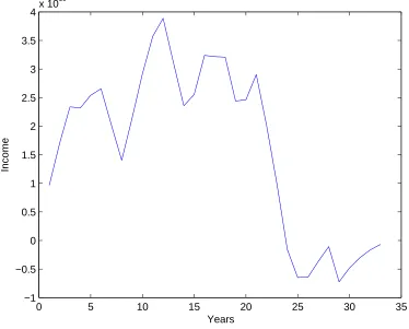
The APEX model produces estimates of exposures inµg/m3_{corresponding to the concentration of PM} 10 a simulated individual is exposed to in a given day according to their activities. The sample of individual exposures is then analyzed to find the mean, maximum, and percentiles of the population exposure distribution. For example, the covariate “P95” is the concentration of PM10a person in the 95th percentile of the exposure distribution experiences. The APEX exposure concentrations are lower than the ambient concentrations of PM10 in the atmosphere, as shown in Figure 1.

2.3 Imputation of Missing Data

Our data set has a large amount of missing values for multiple covariates for various reasons. As our primary objective is to analyze the association between PM10 concentration, APEX and the number of deaths, we dismissed the observations that do not have PM10 measurements. The dismissed PM10values appeared to be missing at random and included approximately 7.8% of the observations. Also, APEX data are only available from January 1, 1994 forward, so only these dates are included. After these two considerations, 2557 daily observations for each city remain.

The average relative humidity information was absent in all observations past January 1, 1998, for both Chicago and Cleveland. Alternate data were obtained through National Climate Data Center (NCDC) website to help complete the data set. Daily minimum and maximum relative humidities were recorded for the majority of days during the 14 year span of observations considered, and the average of the minimum and maximum was computed from these observations to provide an additional measurement. Multiple months were not recorded, but the new data filled in enough of the missing time period to allow analysis to continue. Due to the difference in available measurements from the two sources, the NCDC maximum, minimum, and derived average relative humidity measurements replaced the NMMAPS average relative humidity in our analysis.

2_{http://www.epa.gov/ttn/airs/airsaqs/detaildata/downloadaqsdata.htm} 3_{http://www.census.gov/prod/cen2000/doc/sf1.pdf}

4_{http://www.census.gov/population/www/cen2000/phc-t28.html} 5_{http://transtats.bts.gov}

(7)

0 5 10 15 20 25 30

0

50

100

150

Chicago July 1st 1994 to July 31st 1994

time (one month)

PM

P95 P50 P5 pm10max pm10mean

Figure 1: Ambient PM10concentrations and APEX PM10exposure concentration, Chicago. PM measured in µg/m3_{. P95, P50, and P5 are the concentration of PM}

10a person in the 95th, 50th, and 5th percentile of the population exposure distribution experiences, respectively. pm10max and pm10mean are the maximum and mean daily PM10concentrations.

(8)

0 1000 2000 3000 4000 5000

−20

0

20

40

Chicago site

Time

Ozone

(a) Time Series for Ozone Concetration

(b) Temperature vs. Ozone for Chicago

Figure 2: Ozone Concentrations for Chicago.

(9)

0 1000 2000 3000 4000 5000

−20

0

20

40

Cleveland site (before imputation)

Time

Ozone

(a) Original Time Series

0 1000 2000 3000 4000 5000

−20

0

20

40

Cleveland site (after imputation)

Time

Ozone

(b) Time Series with Imputed Data

Figure 3: Time Series of Ozone Concentrations for Cleveland.

(10)

Predictors Primary reasons for inclusion

Day of the week To allow for different baseline mortality rates within each day of the week

Time To adjust for long-term trends and seasonality

Temperature

To control for the known effects of weather on mortality Dewpoint

Relative humidity Mean CO

To control the potential effects of pollutants on mortality Mean Ozone

Mean SO2 Mean NO2

Table 1: Potential confounding factors in the model

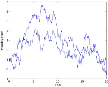
The ozone measurement had systematic missing observations for Cleveland because the city does not monitor ozone levels between November 1 and March 31 each year. We imputed the data from other covariates known to affect ozone concentrations. Because Chicago has a near-complete data set for ozone levels (Figure 2a), it was used to explore general trends between ozone concentration and various meteorological data. A linear regression model appeared appropriate with predictors of maximum relative humidity, average daily temperature, day of the week, daily precipitation, total sunshine, and seasonality. A quadratic term for temperature was included to account for a marked increase in ozone for temperatures over 50 (Figure 2b). Seasonality was accounted for by including a sinusoidal term for time as a predictor. Model fit was checked and the model explained most of the variation in ozone measurement. Missing ozone data for Cleveland was filled in based on this model (Figure 3).

Several other covariates were still missing a small number of randomly distributed observations and were chosen to be deleted. PM2.5 was not collected until March 1998, so we did not consider PM2.5in our analysis due to its absence in the majority of the observations and its inclusion in the atmospheric measurement of PM10. After all omissions, there were 2535 observations for Chicago and 2542 observations for Cleveland.

3 Model Description

Generalized additive models (GAM) [7] were used in our analysis to explore the relationship between the count of deaths as dependent variable, and additive predictors through a nonlinear link function. A log-linear GAM was adopted in this case for the Poisson response – the number of events. Day of the week, temperature, dewpoint, relative humidity, seasonality, mean CO level, mean Ozone level, mean SO2 level and mean NO2 level were included in the model as potential confounding effects (Table 1). To be able to get an overall picture of the air pollution effect on the mortality, we modeled the cardiovascular deaths, respiratory deaths, all cause deaths excluding accident, and chronic obstructive pulmonary disease seperately.

The outcome variable, Yt, is defined as the total number of events of a given type (e.g. cardiovascular

death) at timet. It is assumed to follow a Poisson distribution with meanµt, andYtare independent of given

µt. The GAM model has the form

log(µt) =S(Xt) +βZt,

whereS(Xt) =S(X1t)+S(X2t)+· · ·+S(Xnt), Z= (Z1t, Z2t,· · ·, Zmt)T andβ= (β1,· · ·, βm). The covariates

that are assumed to have linear impact on the log form of the count data are included inZ, while the others are included inX. The non-linear effects of X are modeled using seperate spline functions with various number of knots.

The lag effects of PM10on the number of deaths were also analyzed. For example, the effect of PM10level from the previous day on the mortality of current day was evaluated, refered as ‘one-day lag effect’. In our analysis, no lag, one-day lag, two-day lag, and three-day lag of PM10were fitted in the log linear GAM model seperately to compare the model difference. Akaike’s Information Criterion (AIC), coefficient estimate, and p-value were used as the model selection criterion. AIC, a measure of the goodness of fit for an estimated statistical model, is defined asAIC= 2k−2 log(L), whereLis the maximized value of the likelihood function

(11)

for the estimated model andkis the effective degrees of freedom being estimated, to keep the balance between the goodness of fit and model complexity.

Statistical software R 2.9 was used to carry out the analysis. Package MGCV was used to analyze the Poisson generalized additive models.

4 Simulation Study

In this section, we conduct a simulation study to investigate the potential benefits of accounting for individual exposure in an epidemiological study of air pollution and a health response. We simulate data to closely resemble the Chicago data. The idea of simulation is to generate pollution and response data at the individual level using the APEX distribution and a logistic model. We randomly sample xit for the ith person on the

tth day from the data generated by APEX model (every 5th percentile of estimated PM10 exposure varying from P5 to P95) and thenyitas the response based on these predictors. Consider the logistic regression model

for a response variableyit∼Bernoulli(πit) whereπitis the probability of death on thetthday in the city as

described below.

E(yit) =P(yit= 1|xit) =π(xit) =

exp (β0i+β1ixit)

1 + exp (β0i+β1ixit)

→Logit(π(xit)) = log(

π(xit)

1−π(xit)

) =β0i+β1ixit

β0i ∼N(µ0, σ02) andβ1i ∼N(µ1, σ21). This random-coefficient model allows for heterogeneity in the effect of PM on different individuals in the population.

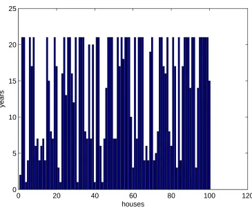
We report the simulation study in which there are d = 120 days and a population size in the city of n= 10000 fors= 100 data sets.

Figure 4: Plot of simulated PM10 exposure data.

In the next step, we generated n=10000 Bernoulli trials,yitwith the probability ofπ(xit). The simulated

response variable for a particular day is the sum of above Bernoulli values, i.e. yt= n X

i=1

yit. So, we studied

the properties of a Poisson random variable regarding our simulated datayt . Figure 4 shows a sample data

set.

(12)

PM10Mean PM10Max P50 P95 Mean Model 1:

β0∼N(−7,0.01) 9 7 6 6 6

β1∼N(0,0) Model 2:

β0∼N(−7,0.01) 18 19 22 20 22

β1∼N(0.0001,0.01) Model 3:

β0∼N(−7,0.01) 73 73 82 79 81

β1∼N(0.01,0.01) Model 4:

β0∼N(−7,0.01) 100 100 100 100 100

β1∼N(0.1,0.01) Model 5:

β0∼N(−7,0.01) 100 100 100 100 100

β1∼N(0.5,0.01)

Table 2: Estimated power for the GLM models.

All the simulations were conducted in R using the GLM to fit the model. We fit the Poisson regression models taking the simulated yt as the response variable and PM10mean, PM10max, P50, P95, and mean

exposure as the predictor. Selecting one variable at a time we find the p-value of including this predictor in the model. Table 2 reports the proportion ofp-values <0.05 for each method, i.e. the power of the method.

There are two things that we are interested in this study Type I error and the power of the test. Type I error is defined by the probability that we reject the null hypothesis if the p-value< 0.05 when the true value of isβ1= 0. Type I error is explored through the first model (whereβ1= 0). The small percentage of rejecting the null hypothesis indicates the small chance to include the predictor variable in the model when there is truly no β1. It can be seen that all of these parameters provide a 6 - 9% chance of rejecting the null hypothesis, slightly greater than the acceptable range (p-value = 0.05). For the power of the test, we look at the probability that we reject the null hypothesis whenβ16= 0. The power of the test is examined by models 2 - 5. The high percentage of rejecting the null hypothesis represents the ability to include the predictor variable in the model. Overall, these five variables have a high chance (>70%) to add to the model when it should truly be in the model. The APEX exposure estimates (P50, P95, and mean) are better predictors in all four models (2–5) than the ambient concentrations (PM10mean and PM10max) since they generally have a higher percentage of rejecting the null hypothesis whenβ16= 0.

5 Results

To determine the appropriate lag model, we considered lag for zero to three days and ranked them according to their AIC value, and whether or not the lag was statistically significant. Our findings were that one day lag was the best model for Chicago, and same day PM10 Cleveland. Because of this we chose to model both cities separately, Chicago with one day lag and Cleveland with no lag. These choices of lag within each city were consistent across all causes of death in each city respectively.

For each city we ran several models, shown in Tables 3 and 4. In both cities we varied our responses to consider different types of death. We also varied the indicator of PM10, including the mean level of PM10 for a given day (pm10mean), the maximum of the hourly measurements of PM10 (pm10max), 50th percentile of the population exposure distribution (P50), the 95th percentile of the population exposure distribution (P95), and the mean of the population exposure distribution (mean).

The predictor that is most commonly considered in epidemiological studies is pm10mean, however we can see from the Table 3 that for the Chicago data set pm10max has smaller AIC for all four of our responses. One plausible explanation for pm10max having a stronger association than pm10mean could be that the death response is triggered only after PM10 has reached some threshold level. In this case the pm10max would be a

(13)

COD AIC RR Log RR P-Values

PM10 Mean Resp 13021.9 1.01 0.011 0.0099

PM10 Max Resp 13018.6 1.01 0.011 0.0022

P50 Resp 13023.1 1.04 0.037 0.0179

P95 Resp 13021.5 1.02 0.021 0.0086

Mean Resp 13022.6 1.04 0.037 0.0140

PM10 Mean CVD 18199.4 1.005 0.005 0.0216

PM10 Max CVD 18195.1 1.01 0.005 0.0045

P50 CVD 18203.3 1.01 0.013 0.0999

P95 CVD 18200.2 1.01 0.009 0.0295

Mean CVD 18202.4 1.01 0.014 0.0691

PM10 Mean COP 10761 1.01 0.011 0.0675

PM10 Max COP 10759.9 1.01 0.011 0.0394

P50 COP 10762.6 1.03 0.031 0.1719

P95 COP 10762 1.02 0.018 0.1146

Mean COP 10762 1.03 0.030 0.1506

PM10 Mean NAD 20401.6 1.006 0.006 <0.0001

PM10 Max NAD 20401.3 1.005 0.005 <0.0001

P50 NAD 20409 1.018 0.018 0.0005

P95 NAD 20402.8 1.011 0.011 0.0001

Mean NAD 20407 1.018 0.018 0.0003

Table 3: Chicago. The relative risk, RR, correlates to a 10_mµg3 increase in PM10. RR =e10 ˆβ. NAD = Non-accidental death. Mean level of PM10for a given day (pm10mean), the maximum of the hourly measurements of PM10(pm10max), 50th percentile of the population exposure distribution (P50), the 95th percentile of the population exposure distribution (P95), and the mean of the population exposure distribution (mean).

good predictor of whether that threshold was reached.

Although pm10max is the best predictor for Chicago, the goal of our study is to determine how well the APEX data predicts each response. From Table 3 we see that P95 is a statistically significant predictor for respiratory death and non-accidental death, and that each model has an AIC value comparable to that of the pm10max predictor. However, P95 does not appear to be a good predictor of COPD or CVD.

For Cleveland, Table 4, P95 is a noticeably better predictor of respiratory and non-accidental death. For the Chicago data the difference between AIC values for the pm10max and P95 models is less than 3 for the respiratory response and less than 1.5 for non-accidental death response, however for the Cleveland data we find that the P95 model has an AIC value 2 less that the pm10max model for the respiratory response and about 5.7 less than the pm10max model for the non-accidental death response. Hence P95 is a better predictor of non-accidental death in Cleveland, and at least as good of a predictor for respiratory death in Chicago and Cleveland, and non-accidental death in Chicago.

Upon analysis we discovered that the principal confounders that are significant to our models are mean temperature, time trend (which accounts for seasonal variation), relative humidity, and in our Chicago models carbon monoxide mean. Table 5 shows the p-values for each of the confounders for eight different models. As we saw above, pm10max and P95 models for respiratory and non-accidental death responses are the most interesting. Hence we only included these eight.

We can see from the table that mean temperature, date, and relative humidity are usually statistically relevant predictors of the respiratory and non-accidental death responses. In Chicago carbon monoxide mean is also a statistically significant predictor.

6 Conclusions

We studied the air pollution and its relationship to the mortality data in 2 selected cities, Chicago and Cleveland. The exposures and ambient are used to compare for fitting the model in each city. One problem we

(14)

COD AIC RR Log RR P-Values

PM10 Mean Resp 7605.7 1.026 0.026 0.0441

PM10 Max Resp 7606.7 1.015 0.015 0.0848

P50 Resp 7602.1 1.094 0.090 0.0063

P95 Resp 7604.6 1.037 0.036 0.0232

Mean Resp 7602.6 1.085 0.082 0.0079

PM10 Mean CVD 11776.1 1.019 0.019 0.0001

PM10 Max CVD 11778.4 1.012 0.012 0.0005

P50 CVD 11785.6 1.027 0.027 0.0443

P95 CVD 11783.2 1.016 0.016 0.0112

Mean CVD 11784.8 1.027 0.027 0.0276

PM10 Mean COP 6286.7 1.031 0.031 0.0663

PM10 Max COP 6287.2 1.02 0.020 0.0918

P50 COP 6282 1.105 0.100 0.0226

P95 COP 6289 1.041 0.040 0.0603

Mean COP 6282.7 1.092 0.088 0.0323

PM10 Mean NAD 13461.1 1.015 0.015 <0.0001

PM10 Max NAD 13464.7 1.009 0.009 0.0001

P50 NAD 13463.3 1.037 0.036 <0.0001

P95 NAD 13459 1.019 0.019 <0.0001

Mean NAD 13461.7 1.036 0.035 <0.0001

Table 4: Cleveland. The relative risk, RR, correlates to a 10_mµg3 increase in PM10. RR=e10 ˆβ.NAD = Non-accidental death. Mean level of PM10for a given day (pm10mean), the maximum of the hourly measurements of PM10(pm10max), 50th percentile of the population exposure distribution (P50), the 95th percentile of the population exposure distribution (P95), and the mean of the population exposure distribution (mean).

found is that there are many missing data, especially in Cleveland data set. The linear regression technique is applied to impute the missing data in Cleveland. In the other hand, we removed the missing data in Chicago as only a few are missing. The results show that the best predictor variables that will be included in the model vary by city to city. The max, ambient, and concentration variables are significant to the model for Chicago data whereas 95th percentile of exposure is only one significant variable for modeling Cleveland. We also investigated an accounting for individual variable by simulation method. The non-accidental deaths are generated by assuming Bernoulli distribution with the probability that was randomly selected from 5th 95th percentile of the exposures of the APEX model. Then, we fitted the data to the Poisson regression model and calculated the proportion that we reject the null hypothesis if p-value ¡ 0.05 when the null hypothesis is true. The simulation results present that the exposure can lead to a 5-10% increase in the power of test.

Several issues concern about the limitations in this study, for example, the small data set, and the variables assumed in the simulation model. First we picked only Chicago and Cleveland to fit the model and did the simulation for Chicago data. It can be extended to additional cities and we also recommend investigating these additional data as well as we did for Chicago. Second, we examine one variable in the simulation at a time which is the percentile of the PM10exposure estimated by APEX model. It is interesting to add one or more variable to the model and also the higher order terms including the polynomial and interaction for the further study. Another issue to concern is that the results of simulation technique rely on the generated data only from the APEX model. It is possible to improve the data by combining the simulated exposures with the actual data.

(15)

Chicago Cleveland

pm10max P95 pm10max P95

resp NAD Resp NAD Resp NAD Resp NAD

Mean Tempeture 2.62e-08 2e-16 1.06e-08 2e-16 0.07 0.039 0.0683 0.0124

Date 7.54e-10 2e-16 7.89e-10 2e-16 0.04 0.0003 0.0431 1.05e-07

Relative humidity 0.0001 1.88e-06 0.0002 0.0001 0.007 0.0158 0.0272 0.0472

COmean 0.0124 0.009 0.013 0.0097 0.38 0.5131 0.4425 0.8706

Table 5: Table ofp-values for each confounder for each model.

References

[1] Dominici, F., Daniels, M., Zeger, S.L., Samet, J.M. (2002). “Air Pollution and Mortality: Estimating Regional and National Dose-Response Relationships.” J. Amer. Statistical Assoc. 97(457):100-111.

[2] Daniels, M., Dominici, F., Samet,J. M., and Zeger, S. L. (2000), “Estimating PM10-Mortality Dose-Response Curves and Threshold Levels: An Analysis of Daily Time-Deries for the 20 Largest U.S. Cities,” American Journal of Epidemiology, 152:397-412.

[3] Schwartz, J. (1994), ”Air Pollution and Daily Mortality: A Review and Meta Analysis,”’ Environmental Research, 64:36-52.

[4] U.S. Environmental Protection Agency (1996), ”Review of the National Ambient Air Quality Standards for Particulare Matters: Policy Assessment of Scien- tific and Technical Information,” OAQPS Staff paper.

[5] McCurdy, T., Glen, G., Smith, L., Lakkadi, Y. (2000). “The National Exposure Research Laboratory’s Consolidated Human Activity Database. J. Exposure Anal. Environ. Epidemiol. 10:566-578.

[6] U.S. Environmental Protection Agency (2008). Total Risk Integrated Methodology (TRIM) - Air Pollutants Exposure Model Documentation (TRIM.Expo / APEX, Version 4) Users Guide and Technical Support Document. U.S. Environmental Protection Agency, Research Triangle Park, NC. EPA-452/B-08-001a,b. http://www.epa.gov/ttn/fera/human apex.html.

[7] Hastie, T.J. and Tibshirani, R.J. (1990).Generalized Additive Models. New York: Chapman and Hall.

[8] Haneuse, S., and Wakefield, J. (2008). “The combination of ecological and case-control data”. J.R. Statist. Soc. B, 70:73-93.

(16)

Dosing Predictions for the Anticoagulant Warfarin

Group Members: Lili Ding

∗

_{, Noory Kim}

†

_{, Mario Morales}

‡

_,

Dale Pearson

§

_{, Jacob Porter}

¶

_{, Maryam Shafahi}

k

Advisors: Alison Motsinger-Reif

∗∗

_{, Micheal Wagner}

††

July 28, 2009

∗_{University of Cincinnati, Cincinnati, OH} †_{Towson University, Towson, MD} ‡_{Hunter College, New York, NY} §_{Texas Tech University, Lubbock, TX} ¶_{University of California, Davis} k_{University of California, Riverside} ∗∗_{North Carolina State, Raleigh, NC}

††_{University of North Carolina at Chapel Hill, Chapel Hill, North Carolina}

(17)

CONTENTS 2

List of Figures

1 published NEJM algorithm . . . 15

2 Frequency of different CYP2C9 variants in OMB population groups . . . 19

3 Univariate analysis of CYP2C9 for different subpopulations . . . 19

4 Univariate analysis of different gene variants for the whole population . . . 20

5 Model performance by race . . . 23

List of Tables

1 Continuous Variables, mean(SD): OMB Categories . . . 5

2 Continuous Variables, mean(SD): Race Reported Categories (count≥50) . . . 5

3 Demographic Variables: OMB Categories . . . 5

4 Demographic Variables: Race Reported Categories (count≥50) . . . 6

5 Genotype Counts: OMB Categories . . . 7

6 Genotype Counts: Race Reported Categories (count≥50) . . . 8

7 Contingency Analysis for OMB Races . . . 10

8 Contingency Analysis for the Koreans . . . 11

9 Contingency Analysis for the Chinese . . . 12

10 Contingency Analysis for the Japanese . . . 13

11 Contingency Analysis for the Malay and Mixed . . . 14

12 NEJM algorithm [6] Performance . . . 16

13 Univariate Analysis for OMB Races . . . 17

14 Univariate Analysis for the Asian Subgroups . . . 18

15 Multivariable Analyses . . . 22

(18)

1 INTRODUCTION 3

1 Introduction

Since its discovery and approval for human use over fifty years ago, Warfarin has become the most widely used oral anticoagulant worldwide, prescribed over 20 million times each year in the United States. It is commonly used to prevent abnormal blood clotting.

Despite its widespread use it ranks among the top ten drugs in the United States associated with serious adverse events, as doses required for safe and effective treatment can vary by a factor of 10 among individuals. [NEJM] Thus traditional methods of establishing an appropriate warfarin dosage level based on clinically measurable data end up using a significant degree of trial and error. This can put patients at risk from life threatening side effects from over-dosage, which can result in hemorrhaging of blood, or under-dosage, which can result in lack of efficacy in preventing those medical conditions for which warfarin is prescribed (such as stroke).

The efficacy of warfarin for an individual is gauged by the standard measure for blood clotting ability is the International Normalized Ratio (INR). The standard target INR range is between 2.0 and 3.0. For some patients achieving a stable level within this target may not occur even after 90 days.

Currently the process for achieving a stable dose for a patient requires often months of a trial and error process, decreasing efficacy and increasing risk of side effect during that time. By improving on the dosing process, the amount of time it take to reach stable dose, and the corresponding risks to patients could be reduced. It has been previously reported that the use of genetic markers within a predictive dosing algorithm could reduce this time.[2, 3, 4, 7]

Many studies have reliably and consistently found that variations in two genes, cytochrome P4502C9 (CYP2C9) and Vitamin K epoxide reductase complex subunit 1 (VKORC1), are significantly correlated with warfarin dose, and the U.S. Food and Drug Administration (FDA) includes this finding on the drug label. 1 _[5]

Recently, the International Warfarin Pharmacogenetics Consortium (IWPC), composed of 21 research groups from around the world, grouped their studies to assemble a collection of data from 5700 patients and derived a global dosing algorithm based on 5052 of those patients. [6] This pharmacogenomic algorithm had two genetic and six clinical predictors, and predicted over 43% of the variation in therapeutic dosing within the study, outperforming a dosing algorithm with only clinical predictors (26%)and a traditional fixed dose approach (0%).

In the current study, we use the data currently available from the IWPC consortium to evaluate several aspects of the performance of the published algorithm. Additionally, we explore the potential of refined dosing algorithms for different racial and ethnic subpopulations in the data, as unique risk factors and genetic back-grounds may change the optimal model within these groups, with the goal of minimizing error in the models for each individual.

1.1 Methods and Results

1.2 Data Cleaning

The current dataset contained and had clinical and genetic information from 5933 patients. We only consid-ered those subjects who successfully reached a stable dose of warfarin, and whose target INR was between 2

1_{That these two genes play a part in the regulation of blood clotting levels has been known since around the early 1990s. The} genes encode proteins involved in the regulation of vitamin K, which is essential for blood clotting. The VKORC1 is part of the Vitamin K epoxide reductase complex which activates vitamin K, thereby increasing blood clotting ability. CYP2C9 is resident in the liver and its metabolism of warfarin deactivates the effect of warfarin on blood clotting.

(19)

1 INTRODUCTION 4

and 3, to be consistent with the approach of the IWPC study, resulting in a total of 5106 individuals available for analysis. An additional 3 patients were excluded from analysis based on inconsistent or unique racial and ethnic identifiers(H”, Black British”, Black African”), resulting in a total of 5103 patients for analysis. The data had already been cleaned substantially to increase consistency among data entries, and we did some further data cleaning. For example, we eliminated some differences in usage of capital letters and hyphens (other” vs. Other”) as well as some variations in terminology (African-American”, African American”,Black or African-American” were all changed to Black”). Additionally, due to deviations from normality, the outcome variable of interest (the therapeutic dose of warfarin), was transformed using a square root transformation.

1.2.1 Subgrouping

The data set had multiple data fields pertaining to race and ethnicity, including “race reported” and “OMB”. We relied primarily on these two variables to generate ethnic and racial subsets of the table. Individuals that appeared to belong to more than one racial category (having been listed under reported race as “Intermediate” or “Other Mixed Race”) were grouped together under “Other”. Not all racial and ethnic groups had sample sizes deemed large enough to justify separate analysis. For example, only 42 patients (0.008%) were classified as “Hispanic”. 2 _{Only groups with a minimum of 50 individuals per group were used for stratifying the}

datasets into groups.

1.2.2 Data Summary

Data was evaluated for the following variables:

• Continuous variables: height, weight, therapeutic warfarin dose, square root of therapeutic dose, target INR, INR reported with stable warfarin dose

• Categorical variables: clinical

– gender, age

– project site, reason for warfarin treatment

– other health conditions:

diabetes, congestive heart failure and or valve replacement

– other medications:

amiodarone, enzyme inducer status(carbamazepine, phenytoin, OR rifampin), aspirin, acetaminophen, simvastatin, atorvastatin (Lipitor), fluvastatin, lovastatin, pravastatin, rosuvastatin,cerivastatin, sulfonamide antibiotics, macrolide antibiotics, anti-fungal azoles, herbal medications or vitamin supplements

• Categorical variables: genetic CYP2C9, VKORC1 SNPs (1639, 497, 1173, 1542, 3730, 2255, 4451)

Tables 1 through 6 display summaries of the majority of variables included in the current dataset. Summary means, standard deviations, proportions, and total counts are included as appropriate for each variable.

(20)

1 INTRODUCTION 5

Variable Whole Data OMB White OMB Black OMB Asian OMB Other

Count 5103 3035 663 958 447

Height (cm) 168.74 (10.29) 171.03 (9.94) 170.44 (10.42) 161.49 (7.74) 166.21 (9.57) Weight (kg) 80.62 (22.09) 84.65 (19.92) 92.36 (27.07) 61.61 (11.74) 76.58 (19.76) Therapeutic Dose 32.90 (17.36) 33.73 (17.83) 41.69 (19.5) 24.59 (11.12) 32.06 (13.72) Warfarine Dose sqrt 5.56 (1.43) 5.63 (1.44) 6.28 (1.49) 4.84 (1.07) 5.53 (1.20) Target INR 2.52 (0.18) 2.54 (0.15) 2.52 (0.13) 2.39 (0.17) 2.66 (0.23) Reported INR 2.43 (0.33) 2.46 (0.32) 2.44 (0.33) 2.32 (0.32) 2.50 (0.37)

Table 1: Continuous Variables, mean(SD): OMB Categories

Variable Chinese Japanese Korean Malay Mixed NA

Count 335 227 259 82 80 464

Height (cm) 162.08 (7.78) 161.46 (8.29) 160.61 (7.58) 161.57 (6.8) 162.88 (9.79) 169.73 (9.61) Weight (kg) 62.28 (12.91) 61.41 (10.41) 59.62 (9.87) 63.69 (13.33) 70.17 (14.17) 87.09 (21.33) Therapeutic Dose 22.81 (10.51) 19.99 (9.03) 28.4 (8.33) 25.69 (9.7) 32.31 (10.93) 32.69 (14.68) Warfarine Dose sqrt 4.66 (1.03) 4.36 (0.97) 5.27 (0.78) 4.97 (0.98) 5.6 (0.98) 5.58 (1.24)

Target INR 2.5 (0) 2.31 (0.25) 2.25 (0) 2.5 (0) 2.77 (0.25) 2.66 (0.12)

Reported INR 2.37 (0.36) 2.31 (0.25) 2.21 (0.3) 2.48 (0.26) 2.61 (0.36) 2.53 (0.34)

Table 2: Continuous Variables, mean(SD): Race Reported Categories (count≥50)

Variable Whole Data OMB White OMB Black OMB Asian OMB Other

Count 5103 3035 663 958 447

Gender female 2234 (43.8%) 1183 (39%) 371 (56%) 448 (46.8%) 232 (51.9%) male 2866 (56.2%) 1852 (61%) 292 (44%) 507 (52.9%) 215 (48.1%) Total Known 5100 (99.9%) 3035 (100%) 663 (100%) 955 (99.7%) 447 (100%)

Age (years) 10-19 13 (0.3%) 6 (0.2%) 2 (0.3%) 2 (0.2%) 3 (0.7%)

20-29 119 (2.3%) 69 (2.3%) 21 (3.2%) 14 (1.5%) 0 (0%)

30-39 230 (4.5%) 103 (3.4%) 49 (7.4%) 51 (5.3%) 15 (3.4%)

40-49 545 (10.7%) 231 (7.6%) 109 (16.4%) 147 (15.3%) 27 (6%)

50-59 1000 (19.6%) 505 (16.6%) 163 (24.6%) 234 (24.4%) 0 (0%) 60-69 1211 (23.7%) 692 (22.8%) 151 (22.8%) 276 (28.8%) 58 (13%) 70-79 1341 (26.3%) 940 (31%) 120 (18.1%) 185 (19.3%) 98 (21.9%)

80-89 597 (11.7%) 465 (15.3%) 42 (6.3%) 34 (3.5%) 92 (20.6%)

90+ 33 (0.6%) 24 (0.8%) 6 (0.9%) 1 (0.1%) 96 (21.5%)

Total Known 5089 (99.7%) 3035 (100%) 663 (100%) 944 (98.5%) 56 (12.5%)

(21)

1 INTRODUCTION 6

Variable Chinese Japanese Korean Malay Mixed NA

Count 335 227 259 82 80 464

Gender female 142 (42.4%) 63 (27.8%) 176 (68%) 41 (50%) 51 (63.8%) 191 (41.2%) male 193 (57.6%) 161 (70.9%) 83 (32%) 41 (50%) 29 (36.3%) 273 (58.8%) Total 335 (100%) 224 (98.7%) 259 (100%) 82 (100%) 80 (100%) 464 (100%)

Age 10-19 1 (0.3%) 0 (0%) 1 (0.4%) 0 (0%) 2 (2.5%) 0 (0%)

20-29 4 (1.2%) 0 (0%) 5 (1.9%) 3 (3.7%) 5 (6.3%) 1 (0.2%)

30-39 21 (6.3%) 2 (0.9%) 19 (7.3%) 3 (3.7%) 8 (10%) 1 (0.2%)

40-49 46 (13.7%) 8 (3.5%) 58 (22.4%) 26 (31.7%) 15 (18.8%) 21 (4.5%) 50-59 79 (23.6%) 39 (17.2%) 89 (34.4%) 18 (22%) 26 (32.5%) 49 (10.6%) 60-69 91 (27.2%) 73 (32.2%) 74 (28.6%) 24 (29.3%) 18 (22.5%) 109 (23.5%) 70-79 81 (24.2%) 76 (33.5%) 11 (4.2%) 4 (4.9%) 5 (6.3%) 172 (37.1%) 80-89 12 (3.6%) 14 (6.2%) 2 (0.8%) 4 (4.9%) 1 (1.3%) 106 (22.8%)

90+ 0 (0%) 1 (0.4%) 0 (0%) 0 (0%) 0 (0%) 5 (1.1%)

Age Total 335 (100%) 213 (93.8%) 259 (100%) 82 (100%) 80 (100%) 464 (100%)

(22)

1 INTRODUCTION 7

Genetic Marker Genotype Whole Data OMB White OMB Black OMB Asian OMB Other

(Count) 5103 3035 663 958 447

CYP2C9 *1/*1 3637 (71.3%) 1907 (62.8%) 577 (87.0%) 835 (87.2%) 318 (71.1%)

*1/*2 738 (14.5%) 619 (20.4%) 38 (5.7%) 1 (0.1%) 80 (17.9%)

*1/*3 467 (9.2%) 336 (11.1%) 23 (3.5%) 75 (7.8%) 33 (7.4%)

*2/*2 55 (1.1%) 49 (1.6%) 0 (0%) 0 (0%) 6 (1.3%)

*2/*3 68 (1.3%) 63 (2.1%) 1 (0.2%) 0 (0%) 4 (0.9%)

*3/*3 19 (0.4%) 15 (0.5%) 0 (0%) 1 (0.1%) 3 (0.7%)

Total Known 4984 (97.7%) 2989 (98.5%) 639 (96.4%) 912 (95.2%) 444 (99.3%)

VKORC1 497 G/G 78 (1.5%) 74 (2.4%) 3 (0.5%) 0 (0%) 1 (0.2%)

G/T 509 (10.0%) 464 (15.3%) 27 (4.1%) 6 (0.6%) 12 (2.7%)

T/T 1281 (25.1%) 637 (21%) 360 (54.3%) 245 (25.6%) 39 (8.7%)

Total Known 1868 (36.6%) 1175 (38.7%) 390 (58.8%) 251 (26.2%) 52 (11.6%)

VKORC1 1173 C/C 928 (18.2%) 455 (15%) 337 (50.8%) 46 (4.8%) 90 (20.1%)

C/T 881 (17.3%) 556 (18.3%) 67 (10.1%) 162 (16.9%) 96 (21.5%)

T/T 975 (19.1%) 207 (6.8%) 7 (1.1%) 732 (76.4%) 29 (6.5%)

Total Known 2784 (54.6%) 1218 (40.1%) 411 (62.0%) 940 (98.1%) 215 (48.1%)

VKORC1 1542 C/C 794 (15.6%) 231 (7.6%) 26 (3.9%) 525 (54.8%) 12 (2.7%)

C/G 1086 (21.3%) 806 (26.6%) 110 (16.6%) 138 (14.4%) 32 (7.2%)

G/G 887 (17.4%) 645 (21.3%) 169 (25.5%) 44 (4.6%) 29 (6.5%)

Total Known 2767 (54.2%) 1682 (55.4%) 305 (46%) 707 (73.8%) 73 (16.3%)

VKORC1 1639 A/A 954 (18.7%) 315 (10.4%) 12 (1.8%) 595 (62.1%) 32 (7.2%)

A/G 1364 (26.7%) 1063 (35.0%) 91 (13.7%) 98 (10.2%) 112 (25.1%)

G/G 1352 (26.5%) 800 (26.4%) 431 (65%) 13 (1.4%) 108 (24.2%)

Total Known 3670 (71.9%) 2178 (71.8%) 534 (80.5%) 706 (73.7%) 252 (56.4%)

VKORC1 2255 C/C 448 (8.8%) 306 (10.1%) 80 (12.1%) 46 (4.8%) 16 (3.6%)

C/T 551 (10.8%) 371 (12.2%) 28 (4.2%) 135 (14.1%) 17 (3.8%)

T/T 657 (12.9%) 116 (3.8%) 10 (1.5%) 524 (54.7%) 7 (1.6%)

Total Known 1656 (32.5%) 793 (26.1%) 118 (17.8%) 705 (73.6%) 40 (8.9%)

VKORC1 3730 A/A 313 (6.1%) 183 (6%) 82 (12.4%) 38 (4%) 10 (2.2%)

A/G 1011 (19.8%) 614 (20.2%) 203 (30.6%) 165 (17.2%) 29 (6.5%) G/G 1320 (25.9%) 465 (15.3%) 102 (15.4%) 734 (76.6%) 19 (4.3%) Total Known 2644 (51.8%) 1262 (41.6%) 387 (58.4%) 937 (97.8%) 58 (13%)

NA 2459 (48.2%) 1773 (58.4%) 276 (41.6%) 21 (2.2%) 389 (87%)

VKORC1 4451 A/A 72 (1.4%) 67 (2.2%) 3 (0.5%) 1 (0.1%) 1 (0.2%)

A/C 271 (5.3%) 227 (7.5%) 33 (5%) 4 (0.4%) 7 (1.6%)

C/C 594 (11.6%) 246 (8.1%) 243 (36.7%) 81 (8.5%) 24 (5.4%)

Total Known 937 (18.4%) 540 (17.8%) 279 (42.1%) 86 (9%) 32 (7.2%)

(23)

1 INTRODUCTION 8

Genetic Marker Genotype Chinese Japanese Korean Malay Mixed NA

(Count) 335 227 259 82 80 464

CYP2C9 *1/*1 285 (85.1%) 218 (96%) 231 (89.2%) 63 (76.8%) 63 (78.8%) 315 (67.9%)

*1/*2 0 (0%) 0 (0%) 0 (0%) 0 (0%) 11 (13.8%) 90 (19.4%)

*1/*3 24 (7.2%) 9 (4%) 28 (10.8%) 7 (8.5%) 5 (6.3%) 47 (10.1%)

*2/*2 0 (0%) 0 (0%) 0 (0%) 0 (0%) 1 (1.3%) 2 (0.4%)

*2/*3 0 (0%) 0 (0%) 0 (0%) 0 (0%) 0 (0%) 7 (1.5%)

*3/*3 0 (0%) 0 (0%) 0 (0%) 0 (0%) 0 (0%) 2 (0.4%)

Total Known 309 (92.2%) 227 (100%) 259 (100%) 70 (85.4%) 80 (100%) 463 (99.8%)

VKORC1 497 G/G 0 (0%) 0 (0%) 0 (0%) 0 (0%) 0 (0%) 4 (0.9%)

G/T 3 (0.9%) 0 (0%) 0 (0%) 0 (0%) 3 (3.8%) 7 (1.5%)

T/T 200 (59.7%) 0 (0%) 26 (10%) 5 (6.1%) 20 (25%) 17 (3.7%)

Total Known 203 (60.6%) 0 (0%) 26 (10%) 5 (6.1%) 23 (28.8%) 28 (6%)

VKORC1 1173 C/C 9 (2.7%) 0 (0%) 0 (0%) 7 (8.5%) 5 (6.3%) 83 (17.9%)

C/T 59 (17.6%) 26 (11.5%) 31 (12%) 36 (43.9%) 2 (2.5%) 91 (19.6%)

T/T 251 (74.9%) 201 (88.5%) 228 (88%) 39 (47.6%) 0 (0%) 27 (5.8%)

Total Known 319 (95.2%) 227 (100%) 259 (100%) 82 (100%) 7 (8.8%) 201 (43.3%)

VKORC1 1542 C/C 250 (74.6%) 201 (88.5%) 23 (8.9%) 37 (45.1%) 3 (3.8%) 33 (7.1%)

C/G 62 (18.5%) 26 (11.5%) 3 (1.2%) 38 (46.3%) 11 (13.8%) 151 (32.5%)

G/G 8 (2.4%) 0 (0%) 0 (0%) 7 (8.5%) 9 (11.3%) 107 (23.1%)

Total Known 320 (95.5%) 227 (100%) 26 (10%) 82 (100%) 23 (28.8%) 291 (62.7%)

VKORC1 1639 A/A 162 (48.4%) 201 (88.5%) 219 (84.6%) 2 (2.4%) 8 (10%) 4 (0.9%)

A/G 36 (10.7%) 26 (11.5%) 30 (11.6%) 0 (0%) 43 (53.8%) 10 (2.2%)

G/G 7 (2.1%) 0 (0%) 0 (0%) 3 (3.7%) 29 (36.3%) 15 (3.2%)

Total Known 205 (61.2%) 227 (100%) 249 (96.1%) 5 (6.1%) 80 (100%) 29 (6.3%)

VKORC1 2255 C/C 9 (2.7%) 0 (0%) 0 (0%) 7 (8.5%) 3 (3.8%) 14 (3%)

C/T 61 (18.2%) 26 (11.5%) 3 (1.2%) 38 (46.3%) 4 (5%) 10 (2.2%)

T/T 250 (74.6%) 201 (88.5%) 23 (8.9%) 37 (45.1%) 0 (0%) 4 (0.9%)

Total Known 320 (95.5%) 227 (100%) 26 (10%) 82 (100%) 7 (8.8%) 28 (6%)

VKORC1 3730 A/A 6 (1.8%) 0 (0%) 31 (12%) 7 (8.5%) 4 (5%) 3 (0.6%)

A/G 62 (18.5%) 26 (11.5%) 0 (0%) 36 (43.9%) 13 (16.3%) 17 (3.7%)

G/G 252 (75.2%) 201 (88.5%) 226 (87.3%) 39 (47.6%) 6 (7.5%) 8 (1.7%)

Total Known 320 (95.5%) 227 (100%) 257 (99.2%) 82 (100%) 23 (28.8%) 28 (6%)

VKORC1 4451 A/A 1 (0.3%) 0 (0%) 0 (0%) 0 (0%) 0 (0%) 3 (0.6%)

A/C 4 (1.2%) 0 (0%) 0 (0%) 0 (0%) 1 (1.3%) 15 (3.2%)

C/C 33 (9.9%) 0 (0%) 26 (10%) 5 (6.1%) 5 (6.3%) 10 (2.2%)

Total Known 38 (11.3%) 0 (0%) 26 (10%) 5 (6.1%) 6 (7.5%) 28 (6%)

Table 6: Genotype Counts: Race Reported Categories (count≥50)

1.2.3 Remarks

Despite data cleaning, there are many caveats in order that are the result of a lack of consistency among groups in (1) selecting patients and in (2) selecting data variables. An example of bias in selecting patients appears in the Korean study, whose 258 patients were all listed as having had a heart valve replacement. The location of consortium members could be partly responsible for the high number of white patients and the low number of Hispanic and African patients. Lack of uniformity in selecting data variables resulted in missing data. Despite a consensus within the IWPC on which variables to include in the overall study, only a few variables had information for all patients in the study.

The therapeutic mean dose for the OMB Asian subpopulation is significantly lower than for other subpop-ulations. Non-genetic factors such as differences in mean weight and target dosage are significantly lower as well, so these could account for at least some of the difference. This lack of consistency makes it difficult to assess the degree that genetic differences have a role in this difference.

(24)

2 TESTS FOR DEMOGRAPHIC DIFFERENCES BETWEEN SUBGROUPS 9

be incorporated could be valuable should a follow up study of this scale be conducted.

2 Tests for Demographic Differences Between Subgroups

To investigate potential clinical and genetic differences between the racial and ethnic subpopulations eval-uated, we performed tests of associations for these demographic variables. All analyses were performed with JMP Version 7.0 (www.jmp.com) and SAS Version 9.1.3 (www.sas.com).

For each racial and Asian subgroup, we compared all of the variables in the published NEJM algorithm [6]. In addition, we compared gender, age, indication for Warfarin treatment, Carbamazepine Tegretol, Pheny-toin Dilantin, Rifampin or Rifampicin, Diabetes, Congestive Heart Failure, Valve Replacements, Aspirin, Ac-etaminophen or Paracetamol, Simvastatin Zocor, Atorvastatin Lipitor, Fluvastatin Lescol, Lovastatin Mevacor, Pravastatin Pravachol, Rosuvastatin Crestor, Cervastatin Baycol, Sulfonamide Antibiotics, Macrolide Antibi-otics, Anti Fungal Azoles and Herbal Medications Vitamins.

Association analysis was performed in JMP software (www.jmp.com). Contrasts between subpopulation were performed with either Chi-square tests of association for categorical demographic variables, or Student’s T tests for continuous outcomes (or nonparametric versions in the case of assumption violations). Two-tailed p-values for obtained for each test. For each test our null hypothesis assumed that there was not a correlation between the row variable and the column variable, and we used a conventional alpha rate of 0.05 as our cut-off for determining statistical significance. Finally, we used Microsoft Excel to plot our p-values for each subgroup.

(25)

White vs. White vs. White vs. Asian vs. Asian vs. Black vs. Variable Black Asian Other Other Black Other

Gender * * * *

Age * * *

Ind. for Warfarin Treatment * * * *

Amiodarone Cordarone * * * * * *

Carbamazepine Tegretol * * * *

Phenytoin Dilantin * * * *

Rifampin or Rifampicin * * * *

Enzyme Inducer Status * *

CYP2C9 *1/*2 * * * *

CYP2C9 *1/*3 * * *

CYP2C9 *2/*2 * *

CYP2C9 *2/*3 * *

CYP2C9 *3/*3

CYP2C9 NA * *

VKORC1 1639 NA * *

VKORC1 1639 A/A * * * * *

VKORC1 1639 A/G * * * *

VKORC1 497 G/T * * * * *

VKORC1 497 G/G * * * * *

VKORC1 497 NA * * * * *

VKORC1 1173 C/C * * * *

VKORC1 1173 C/T * * *

VKORC1 1173 NA * * * * *

VKORC1 1542 C/C * * * * *

VKORC1 1542 C/G * *

VKORC1 1542 NA * * * *

VKORC1 3730 A/A * * * *

VKORC1 3730 A/G * * *

VKORC1 3730 NA * * * * *

VKORC1 2255 C/C * * *

VKORC1 2255 C/T * * *

VKORC1 2255 NA * * * * *

VKORC1 4451 A/A * *

VKORC1 4451 A/C * * * *

VKORC1 4451 NA * * * * *

Diabetes * * * * *

Congestive Heart Failure * * * * * *

Valve Replacement * * * *

Aspirin * * * * *

Acetaminophen * * * *

Simvastatin Zocor * * * *

Atorvastatin Lipitor * * * * * *

Fluvastatin Lescol * * *

Lovastatin Mevacor * * * *

Pravastatin Pravachol * * * * * *

Rosuvastatin Crestor * * * *

Cervastatin Baycol * * * *

Sulfonamide Antibiotics * * * *

Macrolide Antibiotics * * * *

Anti Fungal Azoles * * * *

Herbal Medications * * *

(26)

Korean vs. Korean vs. Korean vs. Korean vs. Korean vs.

Variable Chinese Japanese Malay Mixed NA

Gender * * * *

Age * * *

Ind. for Warfarin Treatment * * * * *

Amiodarone Cordarone * * * *

Carbamazepine Tegretol * * * * *

Phenytoin Dilantin * * * * *

Rifampin or Rifampicin * * * * *

CYP2C9 *1/*2 * *

CYP2C9 *1/*3 *

CYP2C9 *2/*3 *

CYP2C9 NA * *

VKORC1 1639 NA * * * *

VKORC1 1639 A/A * * * *

VKORC1 1639 A/G * * *

VKORC1 497 G/T * *

VKORC1 497 NA * * * *

VKORC1 1173 C/C * * * *

VKORC1 1173 C/T * * *

VKORC1 1173 NA * * *

VKORC1 1542 C/C * * *

VKORC1 1542 C/G * * * * *

VKORC1 1542 NA * * * * *

VKORC1 3730 A/A * * *

VKORC1 3730 A/G * * *

VKORC1 3730 NA * * *

VKORC1 2255 C/C * * * *

VKORC1 2255 C/T * * * *

VKORC1 2255 NA * * * *

VKORC1 4451 A/C *

VKORC1 4451 NA * *

Diabetes * * * * *

Congestive Heart Failure * * * * *

Valve Replacement * * * * *

Aspirin * * * * *

Acetaminophen * * * * *

Simvastatin Zocor * * * * *

Atorvastatin Lipitor * * * * *

Fluvastatin Lescol * * * * *

Lovastatin Mevacor * * * * *

Pravastatin Pravachol * * * * *

Rosuvastatin Crestor * * * * *

Cervastatin Baycol * * * * *

Sulfonamide Antibiotics * * * * *

Macrolide Antibiotics * * * * *

Anti Fungal Azoles * * * * *

Herbal Medications * * * * *

(27)

Chinese vs. Chinese vs. Chinese vs. Chinese vs.

Variable Japanese Malay Mixed NA

Gender * *

Age * * * *

Ind. for Warfarin Treatment * * * *

Amiodarone Cordarone * * * *

Carbamazepine Tegretol * * * *

Phenytoin Dilantin * * * *

Rifampin or Rifampicin * * * *

CYP2C9 *1/*2 * *

CYP2C9 *2/*2 *

CYP2C9 *2/*3 *

CYP2C9 NA * * *

VKORC1 1639 NA * * * *

VKORC1 1639 A/A * * * *

VKORC1 1639 A/G * * *

VKORC1 497 NA * * * *

VKORC1 1173 C/C * * *

VKORC1 1173 C/T * * *

VKORC1 1173 NA * * * *

VKORC1 1542 C/C * * * *

VKORC1 1542 C/G * * *

VKORC1 1542 NA * * *

VKORC1 3730 A/A * *

VKORC1 3730 A/G * * *

VKORC1 3730 NA * * *

VKORC1 2255 C/C * *

VKORC1 2255 C/T * * * *

VKORC1 2255 NA * * *

VKORC1 4451 NA * *

Diabetes * * *

Congestive Heart Failure * * * *

Aspirin * * *

Acetaminophen * * * *

Simvastatin Zocor * * * *

Atorvastatin Lipitor * * * *

Fluvastatin Lescol * * * *

Lovastatin Mevacor * * * *

Pravastatin Pravachol * * * *

Rosuvastatin Crestor * * * *

Cervastatin Baycol * * * *

Sulfonamide Antibiotics * * * *

Macrolide Antibiotics * * * *

Anti Fungal Azoles * * * *

Herbal Medications * * * *

(28)

Japanese vs. Japanese vs. Japanese vs.

Variable Malay Mixed NA

Gender * * *

Age * *

Ind. for Warfarin Treatment * *

Amiodarone Cordarone *

Carbamazepine Tegretol *

Phenytoin Dilantin *

Enzyme Inducer Status * *

CYP2C9 *1/*2 *

CYP2C9 *3/*3 *

CYP2C9 NA * *

VKORC1 1639 NA * * *

VKORC1 1639 A/A * * *

VKORC1 1639 A/G *

VKORC1 497 G/G * * *

VKORC1 497 NA * * *

VKORC1 1173 C/C * * *

VKORC1 1173 C/T * *

VKORC1 1173 NA * * *

VKORC1 1542 C/C * *

VKORC1 1542 C/G * *

VKORC1 1542 NA * *

VKORC1 3730 A/A * *

VKORC1 3730 A/G * *

VKORC1 3730 NA * * *

VKORC1 2255 C/C * *

VKORC1 2255 C/T * *

VKORC1 4451 A/A *

VKORC1 4451 A/C * * *

VKORC1 4451 NA * *

Diabetes * * *

Congestive Heart Failure * * *

Valve Replacement * *

Aspirin * *

Acetaminophen * *

Simvastatin Zocor *

Atorvastatin Lipitor *

Fluvastatin Lescol *

Lovastatin Mevacor *

Pravastatin Pravachol *

Rosuvastatin Crestor *

Cervastatin Baycol *

Sulfonamide Antibiotics *

Macrolide Antibiotics * *

Anti Fungal Azoles * *

(29)

Malay vs. Malay vs. Mixed vs.

Variable Mixed NA NA

Gender *

Age * *

Ind. for Warfarin Treatment * * *

Amiodarone Cordarone * * *

Carbamazepine Tegretol * *

Phenytoin Dilantin * *

Rifampin or Rifampicin * *

CYP2C9 *1/*2 * *

CYP2C9 NA * *

VKORC1 1639 NA * *

VKORC1 1639 A/A * *

VKORC1 1639 A/G * *

VKORC1 497 NA * *

VKORC1 1173 C/C * *

VKORC1 1173 C/T * * *

VKORC1 1173 NA * * *

VKORC1 1542 C/C * *

VKORC1 1542 C/G * * *

VKORC1 1542 NA * * *

VKORC1 3730 A/A * *

VKORC1 3730 A/G * * *

VKORC1 3730 NA * * *

VKORC1 2255 C/C *

VKORC1 2255 C/T * *

VKORC1 2255 NA * *

Diabetes * * *

Congestive Heart Failure * *

Valve Replacement * * *

Aspirin * * *

Acetaminophen * * *

Simvastatin Zocor * * *

Atorvastatin Lipitor * *

Fluvastatin Lescol * *

Lovastatin Mevacor * *

Pravastatin Pravachol * *

Rosuvastatin Crestor * *

Cervastatin Baycol * *

Sulfonamide Antibiotics * *

Macrolide Antibiotics * *

Anti Fungal Azoles * *

(30)

3 MEASURE OF PERFORMANCE OF THE NEJM ALGORITHM BY SUBGROUPS 15

3 Measure of performance of the NEJM algorithm by subgroups

Based on the many demographic differences between the subpopulations (as shown in Tables 7 - 11, we decided to evaluate the performance of the dosing algorithm previously described (reference the NEJM paper). The mean absolute error was used as the measure of fit, based on the published algorithm, shown in Figure 1 .

(31)

4 DOSING PREDICTIONS FOR THE ANTICOAGULANT WARFARIN 16

The Mean Absolute Error (MAE) is a measure of the performance of a forecasting model and is expressed as:

M AE= 1

n n X

i=1

|fi−yi|

= 1

n n X

i=1

|ei|

Where

• n is the size of the dataset used.

• i is the index row indicator of individuals.

• fi is the vector of forecasted values by the algorithm.

• yi is the vector of observed outcomes in the dataset.

• ei is the vector of errors of the model.

For each stratified group, the algorithm was used to generate predicted values for the square root trans-formed therapeutic dose of warfarin. These predicted values were used in calculating the MAE and standard deviation of these errors for each group (shown in Table 1).

Group N Rows MAE (Mean/Std Dev)

Total 5103 0.840 (0.742)

OMB White 3035 0.840 (0.764)

OMB Black 663 0.979 (0.861)

OMB Asian 958 0.786 (0.627)

OMB Other 13 0.666 (0.454)

Korean 259 0.727 (0.486)

Chinese 335 0.761 (0.601)

Japanese 227 0.786 (0.707)

Malay 82 0.983 (0.735)

Mixed 80 0.679 (0.532)

NA 464 0.834 (0.612)

Table 12: NEJM algorithm [6] Performance

This chart shows the MAE for each subpopulation. In addition, this table shows the standard deviation in parenthesis. The main observation of the table is that the MAE observed is similar between OMB groups with more accuracy observed in the OMB Asian group. The variability observed is also very uniform between groups with only one exception in the Korean case which is less variable (0.486).

4 Dosing Predictions for the Anticoagulant Warfarin

4.1 Univariate analysis

(32)

and 14 shows the univariate analysis results, where? indicates a significant association between the predictor and the outcome atαlevel of 0.05. The tables also shows how the predictors affect the outcome differently across subpopulations. For example, patient’sheightis significantly associated with the outcome for the whole population and all the subpopulations except for the Chinese and Malay. The patient’sweight is significantly associated with the outcome for the whole population and all the subpopulations except for the Korean. The presence of genotype variants of CYP2C9 affects the outcome for the whole population, the OMB white, OMB Asian, and OMB Other group, but not for the OMB Black group. It also affects the outcome for the Chinese, Japanese, and NA group, but not for the Korean, Malay, and Mixed group. All seven single nucleotide polymorphisms (SNPs) of the gene VKORC1 have significant impact on warfarin dose for the whole population and the OMB White subpopulation. For other subpopulations, at least one of the seven SNPs are associated with the outcome. It is also worth mentioning that the VKORC1 -4451 consensus SNP has impact on only the OMB White subpopulation.

OMB OMB OMB OMB

Variable Whole White Black Asian Other

Height (cm) * * * * *

Weight (kg) * * * * *

Target INR * *

INR on Reported Therapeutic Dose of Warfarin *

Age * * * * *

Gender * * *

Indication for Warfarin Treatment * * * *

Amiodarone (Cordarone) * * * * *

Carbamazepine (Tegretol) * *

Phenytoin (Dilantin) * *

Rifampin or Rifampicin * *

Enzyme inducer status * *

CYP2C9 * * * *

VKORC1 -1639 consensus * * * * *

VKORC1 497 consensus * * * *

VKORC1 1173 consensus * * * * *

VKORC1 -4451 consensus * *

Diabetes *

Congestive Heart Failure and/or Cardiomyopathy * * *

Aspirin * *

Acetaminophen or Paracetamol (Tylenol) *

Herbal Medications, Vitamins, Supplements * * *

(33)

Variable Korean Chinese Japanese Malay Mixed NA

Height (cm) * * * *

Weight (kg) * * * * *

Target INR *

INR on Reported Therapeutic Dose of Warfarin * *

Age * * * *

Gender * *

Indication for Warfarin Treatment * *

Amiodarone (Cordarone) Carbamazepine (Tegretol) Phenytoin (Dilantin) Rifampin or Rifampicin

Enzyme inducer status *

CYP2C9 * * *

VKORC1 -1639 consensus * * * * *

VKORC1 497 consensus *

VKORC1 2255 consensus * * *

VKORC1 -4451 consensus Diabetes

Congestive Heart Failure and/or Cardiomyopathy

Valve Replacement * *

Aspirin *

Acetaminophen or Paracetamol (Tylenol) Herbal Medications, Vitamins, Supplements

(34)

Figure 2: Frequency of different CYP2C9 variants in OMB population groups

As the gene effects on the Warfarin dosing is the focus of this study, a precise knowledge about the dis-tribution of different gene variants within the various races is required. In Figure 2 the frequency of different CYP2C9 variants (represented as proportions/probabilities), namely *1/*1, *1/*2,*1/*3, *2/*2,*2/*3, *3/*3 among the racial groups is shown. It can be seen that the OMB White and Black groups are significantly different in the probability of CYP2C9 *1/*1. In addition, the OMB Asian and White show different behavior for the CYP2C9 *1/*2 distribution.

Fifteenth mathematical and statistical modeling workshop for graduate students