Reliability Analysis of a Parallel Unit System with Two Cold
Standby Units
Shakeel Ahmad
#1, Gunjan Sharma
*2, Upasana Sharma
*3#Akbar Peerbhoy college of Commerce and Economics, Mumbai, India *
Department of Statistics, Punjabi University, Patiala, India
Introduction
Reliability is the ability of a system to perform its intended function under given circumstances and within specified time interval. The standby systems holds a great importance in the field of reliability engineering. Various reliability models have been used by researchers under different circumstances [1-7]. The standby unit helps the system to sustain in presence of main unit’s failure. Therefore, our study deals with such situation.
The complete system consists of one main unit and two cold standby units. In the beginning, there is one main unit which is in operative state and two cold standby units which are kept spare. The cold standby units come into operation mode whenever there is any fault in main unit and it stops functioning. Both cold standby units starts functioning together as the capacity of both cold standby units to bring out smooth function of complete system is equivalent to that of one main unit. There is only one repairman available to do the job of repair for main as well as cold standby units. Various measures of system effectiveness such as MTSF and Profit are obtained using semi Markov process and Regenerative point technique. The graphical interpretation has also been done for the present study.
Assumptions
1. There are no different repairmen for main unit and cold standby units i.e. there is single repairman facility available.
2. Working of both cold standby systems will keep the system operating.
3. At an instance, only one unit of cold standby system can fail, i.e. Failure in both cold standby units cannot occur simultaneously.
4. Only one failure can occur at a time.
Notations
λ Rate of occurrence of failure in main unit
λ1/ λ2 Rate of occurrence of failure in Ist / IInd cold standby unit
g(t)/ G(t) pdf/ cdf of times to repair the main unit at failed state
g1(t)/ G1(t) pdf/ cdf of times to repair the Ist cold standby unit at failed state
g2(t)/ G2(t) pdf/ cdf of times to repair the II nd
cold standby unit at failed state OI/OII/OIII Ist/ IInd/ IIIrd unit under operation
SII/SIII IInd/ IIIrd unit under cold standby state
FrI/FwrI Ist unit under repair/ waiting for repair
FrII/FwrII IInd unit under repair/ waiting for repair
Abstract
:
The present study deals with the reliability analysis of a parallel unit system with two cold standby units. In the beginning, there is one main unit and two cold standby units. The system remains in operable state until its complete failure and whenever system comes across any halt, both cold standby units start functioning together in order to keep the system operating. There is single repairman available for repair of main as well as cold standby unit. The reliability and profit analysis has been done for the present model. Various measures of system effectiveness such as MTSF and Profit are obtained using semi Markov process and Regenerative point technique.FrIII/FwrII IIIrd unit under repair/ waiting for repair
FRI I
st
unit under repair continuing from the previous state FRII IInd unit under repair continuing from the previous state
FRIII IIIrd unit under repair continuing from the previous state
Transition Probabilities and Mean Sojourn Times
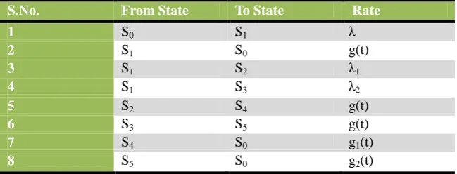
The possible states of the system with current status are provided Table No. I and the transition rates are given in Table No. II. The epochs of entry into states 0, 1, 4 and 5 are regenerative points and thus these are regenerative states. The states 2 and 3 are failed states.
State No. Status S0 OI , SII , SIII
S1 FrI , OII , OIII
S2 FRI , FwrII , SIII
S3 FRI , SII , FwrIII
S4 OI , FrII , SIII
S5 OI , SII , FrIII
Table No. I: Possible States with Status
S.No. From State To State Rate
1 S0 S1 λ
2 S1 S0 g(t)
3 S1 S2 λ1
4 S1 S3 λ2
5 S2 S4 g(t)
6 S3 S5 g(t)
7 S4 S0 g1(t)
8 S5 S0 g2(t)
Table No. II: Transition Rate
Transition Probabilities:
The transition probabilities are given by:
dt t g t e
t dQ dt
t g t e
t dQ
dt t g t dQ dt
t g t dQ
dt t g t dQ dt
t g t dQ
t G t e
t dQ t
G t e
t dQ
dt t e
t g t dQ dt
t e t dQ
) ( ) 1 ) ( ( ) ( )
( ) 1 ) ( ( ) (
) ( ) ( )
( ) (
) ( ) ( )
( ) (
) ( ) ( ) ( )
( ) ( ) (
) ( ) ( ) ( )
(
©
© 1 2
2 ) 3 ( 15 2
1 1 ) 2 ( 14
2 50 1
40
35 24
2 1 2 13 2
1 1 12
2 1 10
01
35 24 2 50 ) 3 ( 15 2 1 2 1 2 13 1 40 ) 2 ( 14 2 1 2 1 1 12 2 1 10 01 ) 0 ( ) 0 ( )] ( 1 [ ) 0 ( )] ( 1 [ ) ( 1 p g p g p p g p g p p g p g p p
By these transition probabilities, it can be verified that
1
1
1
1
1
1
1
50 40 35 24 13 12 10 ) 3 ( 15 ) 2 ( 14 10 01
p
p
p
p
p
p
p
p
p
p
p
The unconditional mean time taken by the system to transit for any regenerative state j, when it is counted from epoch of entrance into that state i, is mathematically stated as –
0 2 3 0 1 2 0 1 3 50 2 40 35 1 24 1 13 12 10 01 ) ( ) ( ) ( , 1 ), 0 ( ' ) ( 0 dt t G k dt t G k dt t G k where k m k m m k m m m m m Thus ij q t ij dQ t ij m
The mean sojourn time in the regenerative state i (μi) is defined as the time of stay in that state before transition
to any other state, then we have -
) 0 ( ) 0 ( ) 0 ( ) ( 1 1 2 5 1 4 3 2 2 1 2 1 1 0 g g g g
Mean Time to System Failure
The expressions for the mean time to system failure (MTSF) are obtained on taking the failed states of the system as absorbing states. By probabilistic arguments, we obtain the following recursive relations for ϕi(t),
c.d.f. of the first passage time from regenerative state i to failed state :
(
)
)
(
)
(
)
(
)
(
)
(
)
(
)
(
)
(
)
(
)
(
)
(
)
(
)
(
0 50 5 0 40 4 13 12 0 10 1 1 01 0t
s
t
Q
t
t
s
t
Q
t
t
Q
t
Q
t
s
t
Q
t
t
s
t
Q
t
)
(
)
(
)
(
0s
D
s
N
s
The mean time to system failure when the system starts from the state 0, is
D N s s s R T s s ) ( 1 lim ) ( lim * * 0 0 0 0
Where R*(s) is the Laplace Transformation of the Reliability R(t). The Reliability R(t) of the system at time 't' can be obtained taking inverse Laplace transform of R*(s) Using L 'Hospital rule and putting the value of ϕ0**
(s) we have
10 1 0
1
)
(
p
D
N
Expected Up-Time of the System
Using the arguments of the theory of regenerative processes, the availability AFi(t), the probability that
the system is up at instant 't' with full capacity given that it entered regenerative state 'i' at time t = 0, is seen to satisfy the following recursive relations.
) ( © ) ( ) ( ) ( ) ( © ) ( ) ( ) ( ) ( © ) ( ) ( © ) ( ) ( © ) ( ) ( ) ( ) ( © ) ( ) ( ) ( 0 50 5 5 0 40 4 4 5 ) 3 ( 15 4 ) 2 ( 14 0 10 1 1 1 01 0 0 t AF t q t M t AF t AF t q t M t AF t AF t q t AF t q t AF t q t M t AF t AF t q t M t AF
Taking Laplace transform of the above equations and solving for AF0 **
(s), we have
)
(
)
(
)
(
1 1 * * 0s
D
s
N
s
AF
The steady state availability of the system is given by
1 1 *
0 0
0
lim
(
(
))
D
N
s
sAF
AF
s
Where ) 3 ( 15 3 ) 2 ( 14 2 1 0 1 ) 3 ( 15 3 ) 2 ( 14 2 1 0 1 2 5 1 4 ) ( 1 0)
(
)
(
)
(
)
(
)
(
)
(
)
(
1 2p
k
p
k
D
p
k
p
k
N
t
G
t
M
t
G
t
M
t
G
e
t
M
dt
e
t
M
t
)
(
©
)
(
)
(
)
(
)
(
©
)
(
)
(
)
(
)
(
©
)
(
)
(
©
)
(
)
(
©
)
(
)
(
)
(
©
)
(
)
(
0 50 5
5
0 40 4
4
5 ) 3 ( 15 4 ) 2 ( 14 0 10 1
1 01 0
t
B
t
q
t
W
t
B
t
B
t
q
t
W
t
B
t
B
t
q
t
B
t
q
t
B
t
q
t
B
t
B
t
q
t
B
The steady state busy period of the system is given by:
) 3 ( 15 3 ) 2 ( 14 2 2
1 2
p
k
p
k
N
D
N
B
R
And D1 is already specified above.
Expected No of Visits of Repairman
Using the probabilistic arguments for regenerative process, the following recursive relation for Vi(t) are
obtained.
)
(
)
)(
(
)
(
)
(
)
)(
(
)
(
)
(
)
)(
(
)
(
)
)(
(
)
(
)
)(
(
)
(
)]
(
1
)[
)(
(
)
(
0 50 5
0 40 4
5 ) 3 ( 15 4
) 2 ( 14 0
10 1
1 01
0
t
V
s
t
Q
t
V
t
V
s
t
Q
t
V
t
V
s
t
Q
t
V
s
t
Q
t
V
s
t
Q
t
V
t
V
s
t
Q
t
V
The steady state expected no. of visits of the repairman is given by:
1
)
0
(
3 31 3
N
N
D
N
V
RAnd D1 is already specified above.
Profit Analysis
The expected profit incurred of the system is -
R
R
C
V
B
C
AF
C
P
0 0
1
2C0 = Revenue per unit up time of the system
C1 = Cost per unit up time for which the repairman is busy in repair
C2 = Cost per visit of the repairman
Graphical Interpretation and Conclusion
2 5
1 4 3
2
2 1 1 0
35 24
50 40
) 3 ( 15 2
1 2 13
) 2 ( 14 2
1 1 12
2 1 10 01
2 2 2 1
1 1
1
1
1
1
1
1
1
1
1
)
(
)
(
)
(
p
p
p
p
p
p
p
p
p
p
e
t
g
e
t
g
e
t
g
t t tT0 (in Hrs.)
λ λ1 = 0.000015 λ1 = 0.000020 λ1 = 0.000025
0.000024 16966908 12817058 10325565
0.000026 15638231 11812254 9515258
0.000028 14500408 10951813 8821391
0.00003 13515213 10206819 8220641.5
0.000032 12653979 9555584 7695515.5
0.000034 11894784 8981530 7232640.5
0.000036 11220585 8471768 6821618.5
0.000038 10617931 8016115.5 6454240
0.00004 10076058 7606437 6123937.5
0.000042 9586259 7236139.5 5825401
Table No. III
The behaviour of MTSF w.r.t. V/s rate of failure of main unit (λ) for different values of rate of failure of Ist standby unit (λ1) has been given in Table No. III. From the table, it can be interpreted that MTSF gets
decreased with the increase in the values of the failure of main unit (λ). It is also been interpreted that with the increase in rate of failure of Ist standby unit (λ1), the MTSF decreases.
PROFIT (in INR)
C0 λ = 0.000032 λ = 0.0032 λ = 0.32
200 -166.168594 -20264.27734 -77926.46875
15200 14833.6543 -5279.737793 -65993.14453
30200 29833.47852 9704.800781 -48059.82031
45200 44833.30078 24689.33984 -33126.5
60200 59833.12109 39673.87891 -18193.17969
75200 74832.9375 54658.41406 -3259.859863
120200 119832.4063 99612.03125 41540.10938
135200 134832.2344 114596.5703 56473.4375
150200 149832.0625 129581.1172 71406.75
165200 164831.875 144565.6406 86340.07813
180200 179831.7031 159550.1875 101273.3906
195200 194831.5313 174534.7188 116206.7188
210200 209831.3438 189519.2656 131140.0469
225200 224831.1719 204503.7969 146073.3594
240200 239831 219488.3438 161006.6719
255200 254830.8125 234472.875 175940.0156
Table No. IV
Table No. IV depicts the behaviour of the profit w.r.t. revenue per unit uptime of the system (C0) for
different values of rate failure of main unit (λ). From the table, it is seen that the profit increases with increase in the values of C0. Also, following conclusions can be drawn:
1. For λ = 0.000032, profit is > or = or < according as C0 > or = or < INR 366.10, i.e. the revenue per unit
uptime of the system (C0) should not be less than INR 366 in order to get positive profit.
2. For λ = 0.0032, profit is > or = or < according as C0 > or = or < INR 20464, i.e. the revenue per unit uptime
of the system (C0) should not be less than INR 20464 in order to get positive profit.
3. For λ = 0.32, profit is > or = or < according as C0 > or = or < INR 78688, i.e. the revenue per unit uptime of
system (C0) should not be less than INR 78688 in order to get positive profit.
References
[1]. Nakagawa, T. (1984), “Optimal Number of Units for a Parallel System,” J Appl Probab., 21(2), pp. 431-436.
[2]. Goyal V. and Murari K. (1985), “Profit consideration of a 2-unit standby system with a regular repairman and 2-fold patience time,” IEEE Trans. Reliab., vol. R-34, p. 544.
[3]. Baohe Su (1997), "On a two-dissimilar unit system with three modes and random check”, Microelectronics Reliab., 37, 1233-1238.
[4]. Parashar, B. and Taneja, G. (2007), “Reliability and profit evaluation of a PLC hot standby system based on a master slave concept and two types of repair facilities”. IEEE Trans. Reliab, 56: 534-539. DOI: 10.1109/TR.2007.903151.
[5]. Eryilmaz, S., and Tank, F., (2012), “On Reliability Analysis of a Two-Dependent-Unit Series System with a Standby Unit,” Appl Math Comput., 218(15), pp. 7792-7797.
[6]. Manocha, A., and Taneja, G., (2015), “Stochastic Analysis of a Two-Unit Cold Standby System with Arbitrary Distribution for Life, Repair and Waiting Times,” Int J Performability Eng., 11(3), pp. 293-299.