R E S E A R C H
Open Access
Mid-knot cubic non-polynomial spline for
a system of second-order boundary value
problems
Qinxu Ding
1and Patricia J.Y. Wong
1**Correspondence:
1School of Electrical and Electronic
Engineering, Nanyang
Technological University, Singapore, Singapore
Abstract
In this paper, amid-knot cubic non-polynomial splineis applied to obtain the numerical solution of a system of second-order boundary value problems. The numerical method is proved to be uniquely solvable and it is of second-order accuracy. We further include three examples to illustrate the accuracy of our method and to compare with other methods in the literature.
Keywords: Cubic non-polynomial spline; Second-order; Boundary value problem; Numerical solution
1 Introduction
We consider a system of second-order boundary value problems of the type
y(x) =
⎧ ⎪ ⎪ ⎨ ⎪ ⎪ ⎩
f(x), a≤x≤c,
g(x)y(x) +f(x) +r, c≤x≤d,
f(x), d≤x≤b,
y(a) =a¯, y(b) =b¯,
(1.1)
with continuity conditions ofyandyatcandd. Here,f andgare continuous functions on [a,b] and [c,d], respectively,r,a¯ andb¯are real finite constants. This type of systems arise in the study of obstacle, unilateral, moving and free boundary value problems [7,9, 10,16,23]. For instance, in modeling an elastic string lying over an elastic obstacle, it has been first shown in [19] that a variational inequality can be transformed to Eq. (1.1) by using the penalty function technique of Lewy and Stampacchia [17].
There are substantial interests on the numerical treatment of the problem (1.1). Noor and Khalifa [19] have used a collocation method with cubic B-splines as basis functions to solve (1.1), while the well-known Numerov method and finite difference schemes based on the central difference have been employed in [22]. Thereafter, Al-Said et al. [5] show that cubic spline method gives numerical solutions that are more accurate than that com-puted by quintic spline and finite difference techniques. The numerical results of [5,19, 22] indicatefirst-orderaccuracy for these methods. In [4], a two-stage method is devel-oped where a finite difference scheme is first employed to obtain the numerical solutions
at mid-knots of a uniform mesh, then a second-order interpolation is used to obtain the numerical solutions at the knots. This method is ofsecond-orderaccuracy. Other proven
second-orderaccurate methods include polynomial spline methods that employ quadratic spline [1], cubic spline [2,3] and quintic spline [6]. The numerical solutions are obtained at mid-knots of a uniform mesh in [1–3], while numerical solutions are obtained at the knots in [6]. These polynomial spline methods use ‘continuous’ spline, and derivatives of the spline are involved in the spline relations. On the other hand,discrete splineuses differences instead of derivatives in the spline relations. In [8], Chen and Wong have de-veloped adeficient discrete cubic splinemethod for (1.1). It is proved that the accuracy of the method is two, and the numerical experiments demonstrate better accuracy over polynomial spline methods.
Besides continuous polynomial splines, non-polynomial splines have also been applied to solve (1.1).Non-polynomial spline, also known as parametric spline [13], depends on a parameterk> 0, and reduces to the ordinary cubic or quintic spline whenk→0. Due to the parameterk, the numerical solutions obtained by non-polynomial splines in the literature are observed to be more accurate than that computed by polynomial splines. In fact, a cubic non-polynomial spline method has been proposed by Khan and Aziz [12] and subsequently by Siraj-ul-Islam and Tirmizi [25] to solve (1.1) at the knots of a uniform mesh. The method is shown to be of order two, and numerical results indicate better ac-curacy over polynomial spline methods. Higher degree non-polynomial splines have also been used in higher-order boundary value problems, for example quartic non-polynomial spline for third-order boundary value problem [24,26], quintic non-polynomial spline for fourth-order boundary value problem [14] and sextic non-polynomial spline for fifth-order boundary value problem [15]. Out of all these work, only [26] gives the numerical solutions of the third-order boundary value problem at mid-knots of a uniform mesh while the rest obtains the numerical solutions at the knots. The methods mentioned so far yield discrete numerical schemes. There are also iterative methods such as Adomian decom-position method [18] and variational iteration method [20]. Both of these methods do not require discretization.
Motivated by the above work especially those involving the use of non-polynomial splines, in this paper we shall develop acubic non-polynomial splinescheme atmid-knots
of a uniform mesh for the problem (1.1). The unique solvability and convergence analysis will be carried out which indicates a second-order accurate method. Finally, three exam-ples will be presented to illustrate the numerical efficiency and the better performance over other methods in the literature.
2 Mid-knot cubic non-polynomial spline method
Let:a=x0<x1<· · ·<xn=b be a uniform mesh of [a,b] withxi=a+ih, 0≤i≤n, whereh=b–an is the step size. Without loss of generality, let
c=3a+b
4 =xn/4 and d=
a+ 3b
4 =x3n/4,
and we require the positive integern,n≥12, to be divisible by 4. Thus, the pointscandd
Define themid-knotsof the meshas
xi–1/2=a+
i–1 2
h, 1≤i≤n. (2.1)
Note that the breakup pointscanddarenotany of the mid-knots defined above, in fact
c∈[xn/4–1/2,xn/4+1/2] andd∈[x3n/4–1/2,x3n/4+1/2].
Throughout the paper, for any functionv(x) we shall denotev(j)(xi) =v(j)
i and likewise
v(j)(x i–1/2) =v
(j)
i–1/2. In the following, we define the cubic non-polynomial spline in terms of
mid-knotsof the mesh. Note that [13] gives a similar definition but in terms of theknots
of.
Definition 2.1 For a given mesh, we sayP(x) is thecubic non-polynomial spline with parameter k(>0) ifP(x)∈C(2)[a,b],P(x) has the formspan{1,x,sinkx,coskx}, and its re-strictionPi(x) on [xi–1/2,xi+1/2], 1≤i≤n– 1 satisfies
⎧ ⎨ ⎩
Pi(xi–1/2) =Si–1/2, Pi(xi+1/2) =Si+1/2,
Pi(xi–1/2) =Di–1/2, Pi(xi+1/2) =Di+1/2.
(2.2)
From the above definition, forx∈[xi–1/2,xi+1/2], 1≤i≤n– 1, we can expressPi(x) as
Pi(x) =aisink(x–xi–1/2) +bicosk(x–xi–1/2) +ci(x–xi–1/2) +di. (2.3)
Using (2.2), a direct computation gives
Pi(x) = –Di+1/2+Di–1/2coskh
k2sinkh sink(x–xi–1/2) –
Di–1/2
k2 cosk(x–xi–1/2)
+
Si+1/2–Si–1/2
h +
Di+1/2–Di–1/2
k2h
(x–xi–1/2) +Si–1/2+
Di–1/2
k2 . (2.4)
Then, using the continuity of the first derivative of the spline, namely, Pi–1 (xi–1/2) =
Pi(xi–1/2), 2≤i≤n– 1, we obtain from (2.4)
Si–3/2– 2Si–1/2+Si+1/2=h2(αDi–3/2+ 2βDi–1/2+αDi+1/2), 2≤i≤n– 1, (2.5) where
α= 1
khsinkh–
1
k2h2, β= 1
k2h2 – coskh
khsinkh. (2.6)
Remark2.1 Whenk→0, we have (α,β)→(16,13) and the cubic non-polynomial spline relation of Eq. (2.5) reduces to the well-known cubic spline relation. Further, for the con-sistency of relation (2.5), we have 2α+ 2β= 1 [13].
We shall approximate a solutiony(x) of (1.1) by the non-polynomial splinePi(x) over the subinterval [xi–1/2,xi+1/2], 1≤i≤n– 1. Hence, it follows from (2.5) that
yi–3/2– 2yi–1/2+yi+1/2=h2
wheretiis the truncation error. By Taylor expansion, the truncation error is found to be
ti=h2(1 – 2α– 2β)yi–1/2+h4
1 12–α
y(4)i–1/2+h6
1 360–
α
12
y(6)i–1/2
+Oh7 , 2≤i≤n– 1. (2.8)
Remark 2.2 Due to the consistency relation 2α+ 2β = 1, (2.8) immediately gives ti=
O(h4), 2≤i≤n– 1. If, in addition, α = 1
12 (which implies β = 5
12), then (2.8) yields
ti=O(h6), 2≤i≤n– 1.
Next, since we approximate a solutiony(x) of (1.1) by the non-polynomial splineP(x), it is natural to set the second derivative of the spline as
Di–1/2=
⎧ ⎪ ⎪ ⎨ ⎪ ⎪ ⎩
fi–1/2, 1≤i≤n4,
gi–1/2Si–1/2+fi–1/2+r, n4+ 1≤i≤3n4,
fi–1/2, 3n4 + 1≤i≤n.
(2.9)
Note that in (2.9), by considering the second derivative at mid-knots, weavoidthe breakup pointscanddat whichyis discontinuous.
Substituting (2.9) into (2.5) yields the following equations: • for2≤i≤n4– 1,
Si–3/2– 2Si–1/2+Si+1/2=h2(αfi–3/2+ 2βfi–1/2+αfi+1/2); (2.10)
• fori=n4,
Sn/4–3/2– 2Sn/4–1/2+
1 –αh2gn/4+1/2 Sn/4+1/2
=h2αfn/4–3/2+ 2βfn/4–1/2+α(fn/4+1/2+r)
; (2.11)
• fori=n4+ 1,
Sn/4–1/2+
–2 – 2βh2gn/4+1/2 Sn/4+1/2+
1 –αh2gn/4+3/2 Sn/4+3/2
=h2αf
n/4–1/2+ 2β(fn/4+1/2+r) +α(fn/4+3/2+r)
; (2.12)
• forn4+ 2≤i≤3n4 – 1,
1 –αh2gi–3/2 Si–3/2+
–2 – 2βh2gi–1/2 Si–1/2+
1 –αh2gi+1/2 Si+1/2
=h2α(fi–3/2+r) + 2β(fi–1/2+r) +α(fi+1/2+r)
; (2.13)
• fori=3n 4,
1 –αh2g3n/4–3/2 S3n/4–3/2+
–2 – 2βh2g3n/4–1/2 S3n/4–1/2+S3n/4+1/2
=h2α(f3n/4–3/2+r) + 2β(f3n/4–1/2+r) +αf3n/4+1/2
• fori=3n4 + 1,
1 –αh2g3n/4–1/2 S3n/4–1/2– 2S3n/4+1/2+S3n/4+3/2
=h2α(f3n/4–1/2+r) + 2βf3n/4+1/2+αf3n/4+3/2
; (2.15)
• for3n
4 + 2≤i≤n– 1,
Si–3/2– 2Si–1/2+Si+1/2=h2(αfi–3/2+ 2βfi–1/2+αfi+1/2). (2.16)
To set up a system ofnequations for the unknownSi–1/2, 1≤i≤n, we need two more equations besides (2.10)–(2.16). Using the method of undetermined coefficients, we ob-tain the following two equations which have truncation errors ofO(h6):
⎧ ⎨ ⎩
2S0– 3S1/2+S3/2=h2(–1201 D0+58D1/2+487D3/2–801D5/2),
2Sn– 3Sn–1/2+Sn–3/2=h2(–1201 Dn+58Dn–1/2+487Dn–3/2–801Dn–5/2).
(2.17)
Sincen≥12, from (2.9) we haveDi–1/2=fi–1/2fori= 1, 2, 3, n– 2, n– 1, n. Hence, the above two equations become
⎧ ⎨ ⎩
2S0– 3S1/2+S3/2=h2(–1201 f0+58f1/2+487f3/2–801f5/2),
2Sn– 3Sn–1/2+Sn–3/2=h2(–1201 fn+58fn–1/2+487fn–3/2–801fn–5/2).
(2.18)
We have now derived themid-knot cubic non-polynomial spline schemewhich comprises Eqs. (2.10)–(2.16) and (2.18) with 2α+ 2β= 1. The solvability of the system and the con-vergence analysis will be tackled in the next section.
3 Solvability and convergence
In this section, we shall establish the unique solvability of the mid-knot cubic non-polynomial spline scheme (2.10)–(2.16) and (2.18) and also conduct a convergence analy-sis. To begin with, we define the norms of a column vectorT= [ti] and a matrixQ= [qij] as follows:
T=max
i |ti| and Q=maxi
j
|qij|.
Letei–1/2=yi–12 –Si–12, 1≤i≤nbe the errors. LetY= [yi–1/2],S= [Si–1/2],W = [wi],
T = [ti] andE= [ei–1/2] ben-dimensional column vectors. The system (2.10)–(2.16) and (2.18) can be written as
AS=W, (3.1)
where
Here,A0,QandGaren×nmatrices given by
A0=
⎛ ⎜ ⎜ ⎜ ⎜ ⎜ ⎜ ⎜ ⎝ 3 –1 –1 2 –1
. ..
–1 2 –1 –1 3 ⎞ ⎟ ⎟ ⎟ ⎟ ⎟ ⎟ ⎟ ⎠ , (3.3) Q= ⎛ ⎜ ⎜ ⎜ ⎜ ⎜ ⎜ ⎜ ⎝ 5 8 7 48 – 1 80
α 2β α
. ..
α 2β α
–801 487 58
⎞ ⎟ ⎟ ⎟ ⎟ ⎟ ⎟ ⎟ ⎠ (3.4)
andG=diag[vi–1/2] where
vi–1/2=
⎧ ⎪ ⎪ ⎨ ⎪ ⎪ ⎩
0, 1≤i≤n 4,
gi–1/2, n4+ 1≤i≤3n4, 0, 3n
4 + 1≤i≤n.
(3.5)
Further,W= [wi] is given by
wi=
⎧ ⎪ ⎪ ⎪ ⎪ ⎪ ⎪ ⎪ ⎪ ⎪ ⎪ ⎪ ⎪ ⎪ ⎪ ⎪ ⎪ ⎪ ⎪ ⎪ ⎪ ⎨ ⎪ ⎪ ⎪ ⎪ ⎪ ⎪ ⎪ ⎪ ⎪ ⎪ ⎪ ⎪ ⎪ ⎪ ⎪ ⎪ ⎪ ⎪ ⎪ ⎪ ⎩
2a¯–h2(– 1 120f0+
5 8f1/2+
7 48f3/2–
1
80f5/2), i= 1,
–h2(αfi–3/2+ 2βfi–1/2+αfi+1/2), 2≤i≤n4– 1, –h2[αf
n/4–3/2+ 2βfn/4–1/2+α(fn/4+1/2+r)], i=n4,
–h2[αfn/4–1/2+ 2β(fn/4+1/2+r) +α(fn/4+3/2+r)], i=n4+ 1,
–h2[α(f
i–3/2+r) + 2β(fi–1/2+r) +α(fi+1/2+r)], n4+ 2≤i≤3n4 – 1, –h2[α(f3n/4–3/2+r) + 2β(f3n/4–1/2+r) +αf3n/4+1/2], i=3n4,
–h2[α(f
3n/4–1/2+r) + 2βf3n/4+1/2+αf3n/4+3/2], i=3n4 + 1,
–h2(αf
i–3/2+ 2βfi–1/2+αfi+1/2), 3n4 + 2≤i≤n– 1, 2b¯–h2(– 1
120fn+ 5 8fn–1/2+
7 48fn–3/2–
1
80fn–5/2), i=n.
(3.6)
It follows from (3.1) that
AY=W+T, (3.7)
where
T=AE. (3.8)
Remark3.1 Noting Remark2.2, we see that, for 2≤i≤n– 1,
ti=
⎧ ⎨ ⎩
O(h4), if 2α+ 2β= 1,
Coupling with the fact that the truncation error in the other two equations of Eq. (2.18) isO(h6), we get
T=
⎧ ⎨ ⎩
O(h4), if 2α+ 2β= 1,
O(h6), ifα= 1 12,β=
5 12.
(3.9)
Lemma 3.1([27]) The matrix A0is nonsingular and
A–10 ≤n
2+ 1
8 =
(b–a)2+h2
8h2 . (3.10)
Lemma 3.2([11]) Let D be a square matrix such thatD< 1.Then(I+D)is nonsingular and
(I+D)–1≤ 1
1 –D. (3.11)
We are now ready to establish the unique solvability and the convergence of the mid-knot cubic non-polynomial spline scheme in the following theorem.
Theorem 3.1 Suppose
K=1 8
(b–a)2+h2gˆ< 1, (3.12)
wheregˆ=maxx∈[c,d]|g(x)|.Then the system(3.1)has a unique solution and
E=Oh2 . (3.13)
Proof Suppose (3.1) has a unique solution, then it can be written as
S=A–1W=A0+h2QG –1
W=A0
I+A–10 h2QG –1W
=I+A–10 h2QG –1A–10 W. (3.14)
By Lemma3.1, the inverseA–1
0 exists, hence for the existence of the unique solutionSit remains to show that (I+A–10 h2QG) is nonsingular.
From the definitions of matricesQandG, it is clear that
Q= 1, G= max
n
4+1≤i≤34n
|gi–1
2| ≤ ˆg. (3.15)
Using (3.10) and (3.15), we find
A–10 h2QG≤h2A–10 · Q · G ≤1
8
(b–a)2+h2gˆ=K. (3.16)
SinceK< 1, it follows immediately from Lemma3.2that (I+A–1
Next, we consider the errorE, which from (3.8) can be written as
E=A–1T=I+A–10 h2QG –1A–10 T.
From (3.9), we note thatT=O(h4) in the general case, i.e., 2α+ 2β= 1. Together with Lemma3.2, (3.16) and (3.10), it follows that
E ≤I+A–10 h2QG –1·A–10 · T
≤ A–10 · T 1 –A–10 h2QG
≤ (b–a)2+h2
8h2(1 –K) O
h4
= K
ˆ
g(1 –K)O
h2
=Oh2 .
This shows that (3.1) is a second-order convergence method in the general case when 2α+ 2β= 1.
On the other hand, for the special caseα= 1 12,β=
5
12, we have from (3.9) thatT=
O(h6). So by using a similar argument as above, we obtainE ≤O(h4), which indicates that (3.1) is a fourth-order convergence method. However, the solution of problem (1.1) exists continuously only up to the second derivative. Therefore, the numerical method is only second-order accurate over the whole interval for the special caseα=121,β=125. Indeed, a similar conclusion can be observed in [4–6,8,12,25]. In summary, the numerical method (3.1) is of second order for allαandβsatisfying 2α+ 2β= 1.
Remark3.2 Other than the two equations in (2.17) which have truncation errors ofO(h6), we can also obtain, by the method of undetermined coefficients, the following two equa-tions, which have truncation errors ofO(h4):
⎧ ⎨ ⎩
2S0– 3S1/2+S3/2=h2(–14D0+D1/2),
2Sn– 3Sn–1/2+Sn–3/2=h2(–14Dn+Dn–1/2).
(3.17)
Sincen≥12, from (2.9) we haveDi–1/2=fi–1/2fori= 1,n. Hence, (3.17) leads to
⎧ ⎨ ⎩
2S0– 3S1/2+S3/2=h2(–14f0+f1/2),
2Sn– 3Sn–1/2+Sn–3/2=h2(–14fn+fn–1/2).
(3.18)
from numerical simulation we notice that the errors obtained by the new scheme are gen-erally larger than that obtained by the original proposed scheme. As such, the original scheme (2.10)–(2.16) and (2.18) is a better choice.
4 Application to obstacle boundary value problem
To illustrate the application of the mid-knot cubic non-polynomial spline scheme (2.10)– (2.16) and (2.18), we consider the following well-known obstacle value problem
–y(x)≥f(x), on= [0,π],
y(x)≥ψ(x), on= [0,π],
y(x) –f(x)y(x) –ψ(x)= 0, on= [0,π],
y(0) =y(π) = 0,
(4.1)
wheref(x) is a given force on the string andψ(x) is the elastic obstacle function.
The problem (4.1) has been considered by many authors. Noor and Khalifa [19] first discussed it using the variational inequality approach and showed that the problem (4.1) is equivalent to the variational inequality problem (also see [7,9,16,21])
ρ(y,v–y)≥ f,v–y, for allv∈C, (4.2)
whereρ(·,·) is a coercive continuous bilinear form andCis the closed convex set given by
C={v∈H01()|v≥ψon}andH01() is a Sobolev space.
Following the idea and technique of Lewy and Stampacchia [17], the variational inequal-ity (4.2) can be written as
y–μ(y–ψ)(y–ψ) =f, 0 <x<π,
y(0) =y(π) = 0,
(4.3)
whereμ(t), known as the penalty function, is the discontinuous function defined by
μ(t) =
⎧ ⎨ ⎩
1, t≥0,
0, t< 0, (4.4)
andψis the given obstacle function defined by
ψ(x) =
⎧ ⎪ ⎪ ⎨ ⎪ ⎪ ⎩
–1, 0≤x≤π
4, 1, π4 ≤x≤34π, –1, 3π
4 ≤x≤π.
(4.5)
From Eqs. (4.3)–(4.5), one obtains the following system of second-order boundary value problems:
y=
⎧ ⎨ ⎩
f, 0≤x≤π4 and34π ≤x≤π,
y+f – 1, π
4 ≤x≤ 3π
4 ,
y(0) =y(π) = 0,
(4.6)
with continuity conditions ofyandyatπ4 and34π.
In Example4.1, we shall consider a well-known special case of the system (4.6) when
f = 0. This special case is first discussed in [19] and subsequently considered in almost every paper on system of second-order boundary value problems.
Example4.1 ([19]) We consider the system (4.6) whenf = 0, i.e.,
y=
⎧ ⎨ ⎩
0, 0≤x≤π4 and34π ≤x≤π,
y– 1, π
4 ≤x≤ 3π
4 ,
y(0) =y(π) = 0.
(4.7)
The analytical solution of (4.7) is given by
y(x) =
⎧ ⎪ ⎪ ⎨ ⎪ ⎪ ⎩
4
γ1x, 0≤x≤
π
4, 1 –γ4
2cosh(
π
2 –x),
π
4 ≤x≤ 3π
4, 4
γ1(π–x),
3π
4 ≤x≤π,
(4.8)
whereγ1=π+ 4cothπ4 andγ2=πsinhπ4+ 4coshπ4.
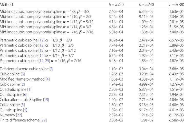
In Table1, we present the maximum absolute errorsE=max1≤i≤n|ei–1/2|obtained from our mid-knot cubic non-polynomial spline scheme for various values ofα andβ, and also the maximum absolute errors obtained from other methods.
From Table1, the numerical results confirm that our method is of second order. Com-pared to the parametric cubic spline method [12,25], our method gives thesmallest errors
for all cases of (α,β). Furthermore, our methodoutperformsall other methods [1–6,8,19, 22] in all cases.
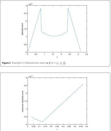
To illustrate graphically, in Figs.1and2, we plot the exact solution, the numerical solu-tion obtained from the mid-knot cubic non-polynomial spline method, and the associated absolute errors when (α,β,h) = (121,125,π
80). It is observed from the figures that this method gives a good approximation to the exact solution.
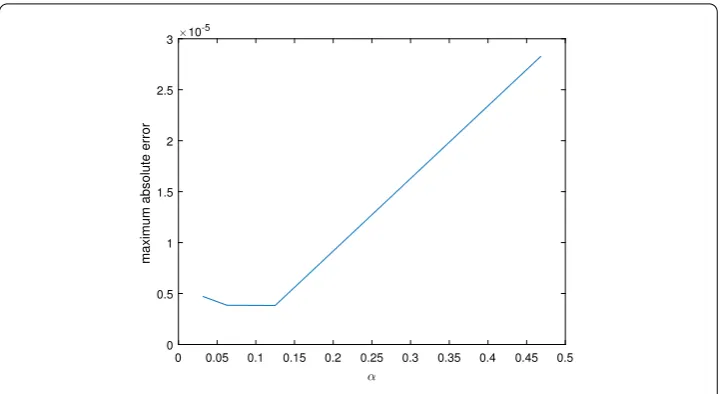
Finally, to investigate the effect ofαon the maximum absolute errorE, in Fig.3we plot the maximum absolute errors for different values ofα∈(0, 0.5) (in steps of321) when
h=80π. It is observed that the minimumEis obtained at aboutα=18.
Table 1 (Example4.1) Maximum absolute errors
Methods h=π/20 h=π/40 h=π/80
Mid-knot cubic non-polynomial splineα= 1/8,β= 3/8 2.40e–04 6.34e–05 1.63e–05 Mid-knot cubic non-polynomial splineα= 1/10,β= 2/5 3.44e–04 9.11e–05 2.34e–05 Mid-knot cubic non-polynomial splineα= 1/12,β= 5/12 4.14e–04 1.09e–04 2.81e–05 Mid-knot cubic non-polynomial splineα= 1/14,β= 3/7 4.64e–04 1.23e–04 3.15e–05 Mid-knot cubic non-polynomial splineα= 1/16,β= 7/16 5.01e–04 1.33e–04 3.40e–05
Parametric cubic spline [12]α= 1/8,β= 3/8 8.62e–04 2.47e–04 6.57e–05 Parametric cubic spline [12]α= 1/10,β= 2/5 7.74e–04 2.21e–04 5.89e–05 Parametric cubic spline [12]α= 1/12,β= 5/12 7.16e–04 2.04e–04 5.43e–05 Parametric cubic spline [12]α= 1/14,β= 3/7 6.74e–04 1.92e–04 5.11e–05 Parametric cubic spline [12,25]α= 1/16,β= 7/16 6.43e–04 1.83e–04 4.87e–05
Deficient discrete cubic spline [8] 1.19e–03 3.04e–04 7.68e–05
Cubic spline [3] 1.26e–03 3.29e–04 8.43e–05
Modified Numerov method [4] 1.65e–03 4.33e–04 1.11e–04
Cubic spline [2] 1.94e–03 4.99e–04 1.27e–04
Quadratic spline [1] 2.20e–03 5.87e–04 1.51e–04
Quintic spline [6] 2.57e–03 7.31e–04 1.94e–04
Collocation-cubic B spline [19] 1.40e–02 7.71e–03 4.04e–03
Cubic spline [5] 1.80e–02 9.13e–03 4.60e–03
Quintic spline [5] 1.82e–02 9.17e–03 4.61e–03
Numerov [22] 2.32e–02 1.21e–02 6.17e–03
Finite difference scheme [22] 2.50e–02 1.29e–02 6.58e–03
Figure 1(Example4.1) Exact solution and numerical solution when (α,β,h) = (1 12,
5 12,
π
80)
Example4.2 We consider the boundary value problem
y=
⎧ ⎪ ⎪ ⎨ ⎪ ⎪ ⎩
2, 0≤x≤π
4,
–y+π162 +74π+ 1, π4 ≤x≤34π,
2, 3π
4 ≤x≤π,
y(0) = 0, y(π) =π 2
2 + 5π
2 + 2.
Figure 2(Example4.1) Absolute error when (α,β,h) = (121,125,80π)
Figure 3(Example4.1) Maximum absolute error for differentαwhenh=80π
Here,f(x) = 2,g(x) = –1 andr=π162 +74π– 1. The analytical solution of (4.9) is given by
y(x) =
⎧ ⎪ ⎪ ⎨ ⎪ ⎪ ⎩
x2+x, 0≤x≤π
4, –√2π
2 sinx–
√
2(π+ 1)cosx+π2
16 + 7π
4 + 1,
π
4 ≤x≤ 3π
4,
x2+x–π2
2 + 3π
2 + 2,
3π
4 ≤x≤π.
(4.10)
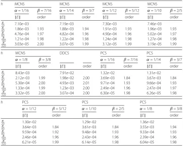
In this example, we focus on comparing the three more accurate methods observed in Table1, namely: (i) mid-knot cubic non-polynomial spline (MCNS), (ii) parametric cubic spline (PCS) [12,25], and (iii) deficient discrete cubic spline (DDCS) [8]. In Table2, we present the maximum absolute errors and the convergence orders of these methods. It is clear that the mid-knot cubic non-polynomial spline scheme obtains thesmallest errors
Table 2 (Example4.2) Maximum absolute errors and convergence orders
h MCNS MCNS MCNS MCNS
α= 1/16 β= 7/16 α= 1/14 β= 3/7 α= 1/12 β= 5/12 α= 1/10 β= 2/5
E order E order E order E order
π
20 7.10e–03 7.19e–03 7.30e–03 7.46e–03
π
40 1.86e–03 1.93 1.88e–03 1.94 1.91e–03 1.93 1.96e–03 1.93
π
80 4.76e–04 1.97 4.82e–04 1.96 4.90e–04 1.96 5.02e–04 1.97
π
160 1.21e–04 1.98 1.22e–04 1.98 1.24e–04 1.98 1.27e–04 1.98
π
320 3.03e–05 2.00 3.07e–05 1.99 3.12e–05 1.99 3.19e–05 1.99
h MCNS DDCS PCS PCS
α= 1/8 β= 3/8 α= 1/16 β= 7/16 α= 1/14 β= 3/7
E order E order E order E order
π
20 8.43e–03 7.91e–02 1.32e–02 1.31e–02
π
40 2.12e–03 1.99 1.98e–02 2.00 3.69e–03 1.84 3.67e–03 1.84
π
80 5.30e–04 2.00 4.93e–03 2.01 9.71e–04 1.93 9.66e–04 1.93
π
160 1.33e–04 1.99 1.23e–03 2.00 2.49e–04 1.96 2.47e–04 1.97
π
320 3.32e–05 2.00 3.07e–04 2.00 6.30e–05 1.98 6.26e–05 1.98
h PCS PCS PCS
α= 1/12 β= 5/12 α= 1/10 β= 2/5 α= 1/8 β= 3/8
E order E order E order
π
20 1.30e–02 1.29e–02 1.36e–02
π
40 3.64e–03 1.84 3.61e–03 1.84 3.55e–03 1.94
π
80 9.59e–04 1.92 9.48e–04 1.93 9.33e–04 1.93
π
160 2.46e–04 1.96 2.43e–04 1.96 2.39e–04 1.96
π
320 6.21e–05 1.99 6.14e–05 1.98 6.04e–05 1.98
Figure 4(Example4.2) Maximum absolute error for differentαwhenh=80π
Next, the effect ofα on the maximum absolute error is illustrated in Fig.4, where we plot the maximum absolute errors for different values ofα∈(0, 0.5) (in steps of 1
32) when
Example4.3 We consider the boundary value problem
y=
⎧ ⎪ ⎪ ⎨ ⎪ ⎪ ⎩
2, 0≤x≤14,
y+163, 14≤x≤34, 2, 34≤x≤1,
y(0) = 1, y(1) =15 8 e
1 2 –1
8.
(4.11)
In this example,f(x) = 2,g(x) = 1 andr= –2916. The analytical solution of (4.11) is given by
y(x) =
⎧ ⎪ ⎪ ⎨ ⎪ ⎪ ⎩
x2+x+ 1, 0≤x≤1
4, 3
2e x–14– 3
16,
1 4≤x≤
3 4,
x2+ (3 2e
1 2–3
2)x+ 3 8e
1 2+3
8, 3
4≤x≤1.
(4.12)
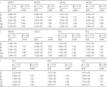
Once again we compare the three better methods arising from Table1, namely: (i) mid-knot cubic non-polynomial spline (MCNS), (ii) parametric cubic spline (PCS) [12,25], and (iii) deficient discrete cubic spline (DDCS) [8]. In Table3, we present the maximum absolute errors of these methods and it is clear that the mid-knot cubic non-polynomial spline schemeoutperformsin all the cases.
In Fig.5, we illustrate the effect ofαon the maximum absolute error. It is observed that the minimumEis obtained at aboutα=18, which is a different value from Example4.2 but is about the same value as in Example4.1.
Table 3 (Example4.3) Maximum absolute errors and convergence orders
h MCNS MCNS MCNS MCNS
α= 1/16 β= 7/16 α= 1/14 β= 3/7 α= 1/12 β= 5/12 α= 1/10 β= 2/5
E order E order E order E order
1
20 5.68e–05 5.68e–05 5.67e–05 5.67e–05 1
40 1.50e–05 1.92 1.50e–05 1.92 1.50e–05 1.92 1.50e–05 1.92 1
80 3.85e–06 1.96 3.85e–06 1.96 3.84e–06 1.97 3.84e–06 1.97 1
160 9.75e–07 1.98 9.74e–06 1.98 9.73e–07 1.98 9.72e–07 1.98 1
320 2.45e–07 1.99 2.45e–07 1.99 2.45e–07 1.99 2.44e–07 1.99
h MCNS DDCS PCS PCS
α= 1/8 β= 3/8 α= 1/16 β= 7/16 α= 1/14 β= 3/7
E order E order E order E order
1
20 5.66e–05 2.60e–04 1.01e–04 1.01e–04 1
40 1.49e–05 1.93 6.50e–05 2.00 2.83e–05 1.84 2.83e–05 1.84 1
80 3.83e–06 1.96 1.63e–05 2.00 7.48e–06 1.92 7.48e–06 1.93 1
160 9.70e–07 1.98 4.06e–06 2.01 1.92e–06 1.96 1.92e–06 1.97 1
320 2.44e–07 1.99 1.02e–06 1.99 4.86e–07 1.98 4.86e–07 1.98
h PCS PCS PCS
α= 1/12 β= 5/12 α= 1/10 β= 2/5 α= 1/8 β= 3/8
E order E order E order
1
20 1.01e–04 1.01e–04 1.01e–04
1
40 2.84e–05 1.83 2.84e–05 1.83 2.84e–05 1.83 1
80 7.49e–06 1.92 7.49e–06 1.92 7.50e–06 1.92 1
160 1.92e–06 1.96 1.92e–06 1.96 1.92e–06 1.97 1
Figure 5(Example4.3) Maximum absolute error for differentαwhenh=801
5 Conclusion
In this paper, we have developed a numerical scheme for a system of second-order bound-ary value problems, which arises from second-order obstacle problem. Our scheme is ob-tained by using cubic non-polynomial spline at mid-knots to avoid the breakup pointsc
andd. We have proved the unique solvability and established convergence order of our scheme. To demonstrate the numerical efficiency and to compare with other methods in the literature, three examples are presented. The numerical results illustrate that our method gives the smallest errors in all the cases.
Acknowledgements
Not applicable.
Funding
Not applicable.
Availability of data and materials
Not applicable.
Competing interests
None of the authors have any competing interests in the manuscript.
Authors’ contributions
All the authors contribute equally to the manuscript. All authors read and approved the final manuscript.
Publisher’s Note
Springer Nature remains neutral with regard to jurisdictional claims in published maps and institutional affiliations.
Received: 4 January 2018 Accepted: 24 September 2018
References
1. Al-Said, E.A.: Spline solutions for system of second-order boundary-value problems. Int. J. Comput. Math.62, 143–154 (1996)
2. Al-Said, E.A.: Spline methods for solving system of second-order boundary-value problems. Int. J. Comput. Math.70, 717–727 (1999)
3. Al-Said, E.A.: The use of cubic splines in the numerical solution of a system of second-order boundary value problems. Comput. Math. Appl.42, 861–869 (2001)
4. Al-Said, E.A., Noor, M.A.: Modified Numerov method for solving system of second-order boundary-value problems. Korean J. Comput. Appl. Math.8, 129–136 (2001)
6. Aziz, T., Khan, A., Khan, I.: Quintic splines method for second-order boundary value problems. Int. J. Comput. Math.85, 735–743 (2008)
7. Baiocchi, C., Capelo, A.: Variational and Quasi-Variational Inequalities. Wiley, New York (1984)
8. Chen, F., Wong, P.J.Y.: Deficient discrete cubic spline solution for a system of second order boundary value problems. Numer. Algorithms66, 793–809 (2014)
9. Cottle, R.W., Giannessi, F., Lions, J.L.: Variational Inequalities and Complementarity Problems: Theory and Applications. Wiley, New York (1980)
10. Crank, J.: Free and Moving Boundary Problems. Clarendon Press, Oxford (1984)
11. Fröberg, C.: Numerical Mathematics, Theory and Computer Applications. Benjamin/Commings, Reading (1985) 12. Khan, A., Aziz, T.: Parametric cubic spline approach to the solution of a system of second-order boundary-value
problems. J. Optim. Theory Appl.118, 45–54 (2003)
13. Khan, A., Khan, I., Aziz, T.: A survey on parametric spline function approximation. Appl. Math. Comput.171, 983–1003 (2005)
14. Khan, A., Noor, M.A., Aziz, T.: Parametric quintic-spline approach to the solution of a system of fourth-order boundary-value problems. J. Optim. Theory Appl.122, 309–322 (2004)
15. Khan Siraj-ul-Islam, M.A., Tirmizi, I.A., Twizell, E.H., Ashraf, S.: A class of methods based on non-polynomial sextic spline functions for the solution of a special fifth-order boundary-value problems. J. Math. Anal. Appl.321, 651–660 (2006) 16. Kikuchi, N., Oden, J.T.: Contact Problems in Elasticity. SIAM, Philadelphia (1988)
17. Lewy, H., Stampacchia, G.: On the regularity of the solution of a variational inequality. Commun. Pure Appl. Math.22, 153–188 (1960)
18. Momani, S.: Solving a system of second order obstacle problems by a modified decomposition method. Appl. Math. E-Notes6, 141–148 (2006)
19. Noor, M.A., Khalifa, A.K.: Cubic splines collocation methods for unilateral problems. Int. J. Eng. Sci.25, 1525–1530 (1987)
20. Noor, M.A., Noor, K.I., Rafiq, M., Al-Said, E.A.: Variational iteration method for solving a system of second-order boundary value problems. Int. J. Nonlinear Sci. Numer. Simul.11, 1109–1120 (2010)
21. Noor, M.A., Noor, K.I., Rassias, Th.: Some aspects of variational inequalities. J. Comput. Appl. Math.47, 285–312 (1993) 22. Noor, M.A., Tirmizi, S.I.A.: Finite difference technique for solving obstacle problems. Appl. Math. Lett.1, 267–271 (1988) 23. Rodrigues, J.F.: Obstacle Problems in Mathematical Physics. North-Holland, Amsterdam (1987)
24. Siraj-ul-Islam, Khan, M.A., Tirmizi, I.A., Twizell, E.H.: Non polynomial spline approach to the solution of a system of third-order boundary-value problems. Appl. Math. Comput.168, 152–163 (2005)
25. Siraj-ul-Islam, Tirmizi, I.A.: Nonpolynomial spline approach to the solution of a system of second-order boundary-value problems. Appl. Math. Comput.173, 1208–1218 (2006)
26. Siraj-ul-Islam, Tirmizi, I.A., Khan, M.A.: Quartic non-polynomial spline approach to the solution of a system of third-order boundary-value problems. J. Math. Anal. Appl.335, 1095–1104 (2007)