28
ANALYTICAL DESIGN OF CGPC-BASED PID CONTROLLERS FOR
COMMONLY ENCOUNTERED ENGINEERING SYSTEMS
Osunleke, A.S., Bamimore, A., Sogunle, O. and Taiwo, O.
Process Systems Engineering Laboratory, Department of Chemical Engineering Obafemi Awolowo University, Ile-Ife, Osun State, Nigeria
E-mail: [email protected]
ABSTRACT
The traditional PID controllers have continued to be the most widely implemented control technique in the industries for many years because of its structural simplicity and its transparent tuning rules. In this work, an analytical design method for PID controllers based on continuous generalized predictive control (CGPC) law is proposed. The design method consists of two steps. The first step entails tuning a CGPC system to obtain a satisfactory closed-loop response. Thereafter a truncated Maclaurin series is employed to approximate the designed CGPC law. Four simulation examples are used to demonstrate the effectiveness of the proposed method. The four examples used are the commonly encountered engineering systems which range from a first order plus time delay system, a second order plus time delay system, a third order system and a non-minimum phase system which has been known to be very problematic to control. The simulation results obtained showed that the proposed CGPC-based PID controllers provided good set-point tracking and disturbance rejection and compared favourably well with PID controllers designed by Ziegler-Nichols and Direct-Synthesis methods. The controllers are also found to be robust as indicated by the small values of computed sensitivity peak.
Keywords: CGPC, PID controller, Direct Synthesis (DS), Ziegler-Nichols (ZN), Tyreus-Luyben (TL)
1. INTRODUCTION
Despite the wide development of advanced control methods, the PID controllers are still commonly used in industry for its structural simplicity and design rules of thumb. The control design problem of this research work involves the approximation of the continuous time version of the generalised predictive control (GPC) algorithm - Continuous time generalised predictive control (CGPC) by a proportional-integral-derivative (PID) controller for the control of commonly encountered engineering systems. Since Clarke et al.
(1987)derived the formula for the GPC controller in discrete form and Demircioglu and Gawthrop (1988) derived its continuous time version, many new predictive control methods based on the GPC approach have been presented (Clarke and Scattolini, 1991; Demircioglu and Gawthrop, 1991; Demirciouglu, 1991) and certain aspects of theoretical analyses of the stability and robustness of the GPC can be found (Wellsted and Zarrop, 1991; Camacho and Bordons, 1991; Deng et al., 2003; Osunleke, 2010). Several successful applications in the chemical industry processes have been reported, which have clearly highlighted the merits of the method. Very recently, Osunleke
(2010) incorporated an anti-windup and
disturbance rejection capability scheme known as robust anti-windup generalised predictive control into the Demircioglu and Gawthrop algorithm. Existing works have shown that a discrete version of a generalised predictive control (GPC) based PID has been derived. The different authors have used different methods in achieving these objectives. Cheng et al. (2003) presented a GPC-based PID with a cost function different from the known GPC cost function to include the proportional, integral, and derivative constants for the PID tuning. Miklovicova and Mrosko (2003) presents a GPC-based PID controllers design by comparing the GPC closed loop with the PID closed loop, deriving the conditions for equivalence to obtain the tuning constants. All these GPC-PID designs have only been presented in the discrete time domain.
29
methods to verify the effectiveness of the proposed system.
2. THE CGPC DESIGN ALGORITHM
Various predictive control algorithms differ in the model used for prediction. The CGPC algorithm uses transfer function model in the form expressed in equation (1) for prediction purposes;
( ) = ( ) ( ) ( ) +
( )
( ) ( ) (1)
A(s), B(s), C(s) are polynomials in Laplace operator, s, with degree n, m, n-1, respectively. Y,
U, and V are the system’s output, input, and disturbance input, respectively. C is usually chosen as a design polynomial having all roots in the left half plane.
The detail of CGPC algorithm will not be derived here as that is available in Demircioglu and Gawthrop(1991)or in its anti-wind up scheme in Osunleke (2010).
The CGPC control law can be obtained by minimizing the cost function;
2 1
2 1
* 2
* 2
0
[ ( , ) * ( , )]
[ ( , )]
T r T
T T r
J y t T w t T dT
u t T dT
(2)
where
∗( , ) = ∗( + ) − ( ) (3)
∗( , ) = ( )
! (4) T1= minimum prediction horizon
T2= maximum prediction horizon λ= control weighting
=control order
Note thatT1, T2, and Nu are all tuning parameters; they can be used to achieve the desired closed-loop response.
The minimization of J in equation (2) results in the control law:
( ) = [ ( ) − ( )] − ( ) ( ) ( ) −
( )
( ) ( ) (5) Where is a scalar gain, Fc and Gc are polynomials.
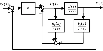
The feedback structure of this CGPC control law as given by equation (5) is illustrated in Figure 1
Fig. 1: The feedback system of CGPC
3. DERIVATION OF PI/PID CONTROLLER FROM CGPC CONTROL LAW
The block diagram in Fig. 1 for the implementation of CGPC control law in a closed loop system can
easily be converted into a conventional feedback system shown in Figure2 through block diagram algebra and transformation, thus giving:
( ) = ( ) ( )
( ) ( ) + ( ) ( ) + ( ) ( ) (6)
Fig 2: The conventional feedback control system
If the derived CGPC control law above is approximated by PID controller, we have
( ) ≅ ( ) = + + (7)
× ( ) ≅ + +
Let ( ) = × ( )
Thus
( ) = + + (8) By expanding f(s) into a Maclaurin series up to the second term, we have
(0) + (0) + 0.5 (0) = + + (9) By equating coefficients, we have
= (0) (10) = (0) (11) = 0.5 (0) (12)
4. SIMULATION RESULTS
Four simulation examples are used to demonstrate the effectiveness of the proposed CGPD-based PID controller. In addition to designing PID controllers based on CGPC control law for each of the examples considered, the controllers were also designed using Direct Synthesis (DS), Internal Model Control (IMC), Ziegler-Nichols (ZN) and Tyreus-Luyben tuning rules.
For comparison purposes, the following robustness and performance metrics were used for assessment.
Robustness Metric: The peak value of the sensitivity function, Ms, is chosen as a measure of system robustness. This has been used widely by various researchers (Chen and Seborg, 2002). Recommended values of Ms are typically in the range of 1.2 – 2.0.
Performance Metrics: Two indices were used to evaluate controller performance. The integrated absolute error (IAE) is defined as:
= ∫ | ( ) − ( )| (13) The total variation of the manipulated input u is used to evaluate the required control effort. The total variation has been widely acclaimed as a good measure of the “smoothness” of a control signal, and it should be as small as possible. It is given by:
-+ ( )
( ) ( ) ( ) +
−
( )
− +
+ + +
-( ) ( ) ( ) ( )
−
( )
( ) ( ) ( )
30
= | ( + 1) − ( )| (14)
4.1 Example 1: First Order Plus Time Delay System
Consider the processdescribed by the transfer function
( ) =
+ 1 (15) Using first order pade approximant, we have
( ) = − + 8
+ 9 + 8 (16) The disturbance model for CGPC algorithm is chosen as ( ) = + 1, and the tuning parameters are selected as
T1=0,T2=1,P=1,Ny=3,Nu=1.5. The CGPC control law is obtained as:
( ) =5 + 50 + 85 + 40
+ 19 + 18 (17)
Fig. 3: Simulation results for Example 1
CGPC-PID controller was then obtained from (14) using equations (9) – (12).
The controller parameters and the performance metrics computed for CGPC law, CGPD-PID, DS-PID and ZN-DS-PID are summarised in Table 1. All the controllers were found to be robust as measured by Ms which is less than 2 for all of them.
Figure 3 shows the simulation results obtained as a result of introducing unit step changes in the set point (as t=0) and in the disturbance (at t=4 sec). CGPC-PID approximated well the CGPC control law and provides a faster response than DS-PID and ZN-PID, with smoother control signal. The DS-PID and ZN-PID responses are a little bit oscillatory. They however provide faster responses to disturbance than CGPC-PID. The computed IAE and TV values corroborate all these claims.
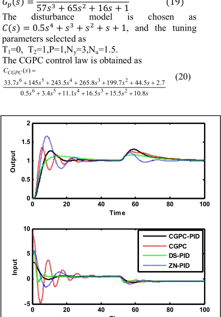
4.2 Example 2: Second Order Plus Time Delay System
Consider a second order plus time delay system described in Seborget al.(2004).
( ) = 2
(10 + 1)(5 + 1) (18) Using optimal model reduction (Taiwo, 1999; Osunleke et al., 2007), equation (18) is approximated to
( ) = 2
57 + 65 + 16 + 1 (19)
The disturbance model is chosen as
( ) = 0.5 + + + + 1, and the tuning parameters selected as
T1=0, T2=1,P=1,Ny=3,Nu=1.5. The CGPC control law is obtained as
6 5 4 3 2
6 5 4 3 2
33.7 145 243.5 265.8 199.7 44.5 2.7
0.5 3.4 11.1
(
16.5 15.5 10.
)
8
CGPC
s s s s s s
s s s
C s
s s s
(20)
Fig. 4: Simulation results for Example 2
CGPC-PID controller was then obtained from (17) using equations (9) – (12).
The controller parameters and the performance metrics computed for CGPC law, CGPC-PID, DS-PID and ZN-DS-PID are summarised in Table 2. CGPC law, DS-PID and CGPC-PID were found to be robust while ZN-PID was clearly not.
Figure 4 shows the simulation results obtained as a result of introducing unit step changes in the set point (as t=0) and in the disturbance (at t=50sec). CGPC-PID approximated well the CGPC control law and provide a faster response than DS-PID and ZN-PID, with smoother control signal though with a little bit of overshoot. The ZN-PID response is quite oscillatory. CGPC-PID however degraded a little bit in terms of disturbance rejection. The computed IAE and TV values corroborate all these claims.
0 1 2 3 4 5 6 7 8
0 0.5 1 1.5
Tim e
O
u
tp
u
t
CGPC-PID
CGPC DS-PID ZN-PID
0 1 2 3 4 5 6 7 8
-2 0 2 4 6
Tim e
In
p
u
t
0 20 40 60 80 100
0 0.5 1 1.5 2
Tim e
O
u
tp
u
t
0 20 40 60 80 100
-5 0 5 10
Tim e
In
p
u
t
31
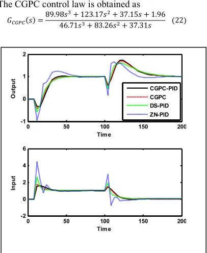
4.3 Example 3: Non-Minimum Phase
System
Consider the non-minimum phase system taken from Bequette
( ) = ( ) = −9 + 1
(15 + 1)(3 + 1) (21) The disturbance model for the CGPC algorithm is chosenas = + 1, while the tuning parametersare chosen as
T1=8,T2=25,P=1,Ny=20,Nu=0.5 The CGPC control law is obtained as
( ) =89.98 + 123.17 + 37.15 + 1.96 46.71 + 83.26 + 37.31 (22)
Fig. 5: Simulation Result for Example 3
CGPC-PID controller was then obtained from (19) using equations (9) – (12).
The controller parameters and the performance metrics computed for CGPC law, CGPD-PID, DS-PID and ZN-DS-PID are summarised in Table 3. All the controllers were found to be robust as measured by Ms which is less than 2 for all of them. Figure 5 shows the simulation results obtained as a result of introducing unit step changes in the set point (as t=0) and in the disturbance (at t=100 sec). CGPC-PID approximated well the CGPC control law and provide a faster response than DS-PID and ZN-PID, with smoother control signal. ZN-PID however performed better than all of them in terms of disturbance rejection. The computed IAE and TV values support all these claims.
4.4 Example 4: Laboratory-Scale
Experimental Three Tank System
Consider a laboratory scale experimental three tank system housed in the process systems engineering laboratory.
Fig. 6: Laboratory-Scale Experimental Three-Tank-System
The Three tank system is originally designed as a two-inputs two outputs system. With pump 2 turned off and level 2 considered as the only controlled variable, the system can be considered as a Single input single output system. The process model is thus obtained as:
( ) = ℎ = 0.216
5.55 × 10 + 3.42 × 10 + 497.39 + 1 (23) The disturbance model for the CGPC algorithm is
chosen as = + + + + 1, and the tuning
parameters are T1=0, T2=500,P=1,Ny=12,Nu=6. The CGPC control law is obtained as
( ) =
88.4 + 93.9 + 93.9 + 93.9 + 5.5 + 0.08 + 0.00016
+ 1.1 + 1.1 + 1.1 + 0.08 + 0.0024 (24)
Fig. 7: Simulation Result for Example 4
0 500 1000 1500 2000
4 4.5 5 5.5 6 6.5
Tim e
O
u
tp
u
t
CGPC-PID CGPC TL-PID
ZN-PID
0 500 1000 1500 2000
0 20 40 60 80 100
Tim e
In
p
u
t
0 50 100 150 200
-1 0 1 2
Tim e
O
u
tp
u
t
CGPC-PID CGPC DS-PID ZN-PID
0 50 100 150 200
-2 0 2 4 6
Tim e
In
p
u
t
q2
d2 d3
d1 q20
q13 q32
Tank 1 Tank 3 Tank 2
h1
h3
h2 Pump
2
q1
Pum
p
32
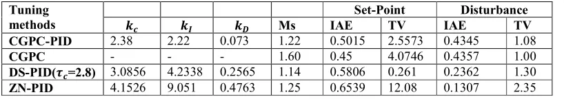
Table 1: PID controller settings for Example 1: First Order Plus Delay System Tuning
methods
Set-Point Disturbance
Ms IAE TV IAE TV
CGPC-PID 2.38 2.22 0.073 1.22 0.5015 2.5573 0.4345 1.08
CGPC - - - 1.60 0.45 4.0746 0.4357 1.00
DS-PID( =2.8) 3.0856 4.2338 0.2565 1.14 0.5806 0.261 0.2362 1.30
ZN-PID 4.1526 9.051 0.4763 1.25 0.6539 12.08 0.1307 2.35
Table 2: PID controller settings for Example 2: Second Order Plus Delay System
Tuning methods Set-point Disturbance
Ms IAE TV IAE TV
CGPC-PID 3.76 0.25 6.35 2.08 9.86 7.78 3.93 1.75
CGPC - - - 1.32 11.88 12.00 4.03 1.39
DS-PID( =0.5) 5 0.333 16.65 1.9 9.51 11.16 3.04 2.63
ZN-PID 4.72 0.8096 6.8912 2.365 10.15 16.74 1.75 2.98
Table 3: PID controller settings for Example 3: Non-Minimum Phase System Tuning
methods
Set-Point Disturbance
Ms IAE TV IAE TV
CGPC-PID 0.879 0.0524 0.637 0.7 19.88 2.1902 23.34 1.8611
CGPC - - - 1.95 19.04 2.7671 23.43 1.9199
DS-PID( =5) 0.947 0.0526 2.3684 0.125 19.60 3.2630 23.29 3.0127
ZN-PID 1.2 0.0988 3.6431 0.173 21.34 9.5058 17.44 6.0517
Table 4: PID controller settings for Example 4: Laboratory Scale Three-Tank-System Tuning
methods
Set-Point Disturbance
Ms IAE TV IAE TV
CGPC-PID 16.4 0.03712 153.5 3.2 168.4 16.26 255.9 36.33
CGPC - - - 1.45 114.6 101.68 146.5 72.07
ZN-PID 80.65 0.7676 2118.70 2.3 231.1 245.74 115.6 225.5
TL-PID 61.1 0.1322 2038.3 2.325 128.2 87.01 89.8 100.9
CGPC-PID controller was then obtained from (21) using equations (9) – (12).
The controller parameters and the performance metrics computed for CGPC law, CGPD-PID, TL-PID and ZN-PID are summarised in Table 4. CGPC law is found to have a lower value of Ms than others.
Figure 5 shows the simulation results obtained as a result of implementing the controllers on the nonlinear SIMULINK model of the system. Step changes in the set point at t=0 and in the disturbance at t=1000 seconds simulated as a leak of size 30 cm3/sec in tank 1 and sustained for 100 seconds, were introduced. CGPC-PID approximated well the CGPC control law and provide a faster response than ZN-PID which was quite oscillatory.
CONCLUSION
We have presented in this work an analytical method of designing CGPC-based PID controllers. The comparison made in simulation between the original CGPC law and the approximated PID controller showed that Maclaurin series give a good approximation of the CGPC law. The simulation results obtained on application of the
proposed design method on the four selected examples and comparing with DC-PID, T-L PID and Z-N PID controllers showed the effectiveness of the method.
REFERENCES
Camacho, E. F. and Bordons, C., “Model predictive control.” Springer-Verlag, London, 2004.
Camacho, E.F., and Bordons, C., “Pre computation of generalised predictive self tunning controller”, IEEE trans. of Automatic control, 36: 852-859, 1991.
Clarke, D.W., Mohtadi, C., and Tuffs, P.S., “Generalized Predictive Control”, Automatica, 23(1):137-164, 1987.
Clarke, D. W. and Scattolini,R., “Constrained receeding-horizon predictive control”, IEEE proceedings-D, 138(4): 347-354, 1991.
Chen, D., and Seborg, D. E. “PI/PID Controller Design Based on Direct Synthesis and Disturbance Rejection”, Ind. Eng. Chem. Res. 41:4807-4822, 2002.
33
Structure”. Chinese Journal Chemical Engineering, 55-61, 2003.
Demirciouglu, H., “constrained continuous time generalised predictive control”, IEEE proceedings of control theory and applications, 146(5):470-475, 1991.
Demircioglu, H., and Gawthrop, P.J., “Continuous time
generalised predictive control (CGPC)”,
Automatica, 27(1):55-74, 1991.
Tsang, T. T. and Clarke, D.W., “Generalised Predictive Control with input constraints”, IEEE proceedings-D, 135(6), 451-460, 1988.
Deng, M., Inoue, A., Yanou, A., and Hirashima, H. “Continuous time anti wind up generalised predictive control of non-minimum phase process with input constraint”, Proceeding of the 42nd IEEE CDC, 4457-4462, 2003.
Miklovicova, E., and Mrosko, M., “Predictive PID control”, International Conference of Cybernetics and Informatics, VYSNA BOCA, Slovak, 10-13,2010.
Osunleke, A.S.,”Robust anti wind generalised predictive control design for systems with input constraints and disturbances”. Unpublished PhD. thesis, the
Graduate School of Natural Science and
Technology, Okayama University, Japan, 2010.
Osunleke, A. S., Taiwo, O. and Hossam, A. G.
“OPTIMRED: An Application Package for
Computation of Optimal Model Reduction”, Proceedings of the 2nd International Conference on Innovation Computing, Information and Control, Kumamoto, Japan (CD-ROM), ISBN: 0-7695-2882-1, 2007.
Seborg D.E., Edgar T.F., Mellichamp D.A. “Process dynamics and control”,John Wiley and Sons Inc., New York, 2004.
Taiwo, O. “Cheap Computation of Optimal Reduced-order Models for Systems with Time-delay”, Journal of Process Control, 9:365-371, 1999. Wellsted and M.B. Zarrop,“Self-tuning systems”, John
Wiley & Sons, 1991.
Yang Xi-yun, Xu Da-ping, Liu Yi-bing and Han Xiao-juan. “Study on strategy of superheated steam temperature control using multi-model predictive functions”, Journal of Power Engineering, 2005. Ziegler J.G. and Nichols N.B. “Optimal setting for