Philippine
Export
Efficiency
and
Potential:
An
Application of Stochastic Frontier Gravity Model
Roperto S. Deluna Jr
1*, and Edgardo D. Cruz
21*,2School of Applied Economics,University of Southeastern Philippines, Davao City, 8000, Philippines
Trade across regions and borders are considered important in improving welfare of people. The Philippines is one of the oldest economies in the world, however, for more than a century it experienced severe trade deficit. This could be due to domestic rigidities and rigidities of its trading partners. This study is focused on examining export efficiency and potential based on trading partner’s characteristics using new approach of measuring export potential. The study employed the Stochastic Frontier Gravity Model that measures potential from the frontier unlike the usual measure of gravity model using OLS that measure potential from the mean.
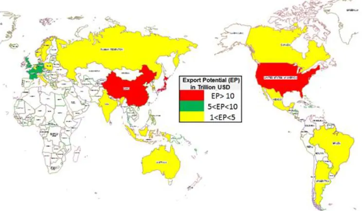
Results show that merchandise export flows of the Philippines is significantly affected by income, market size of the importing partner and the distance between them. The technical efficiency for all countries ranged from 38 to 42%. Countries with larger markets emerged as high export potentials such as USA, China and Japan with potentials ranging from 10 to 30 Trillion US dollars. These potentials have been variable. Results of technical inefficiency model reveal that these potentials are increased by membership of the Philippines to ASEAN, APEC and WTO. Reduction of corruption and freer labor market in the importing country enhanced export potential of Philippine merchandise exports. Commonality of language also enhanced this potential.
Keywords: Merchandise exports, gravity model, stochastic frontier, philippine export potential, PEDP
JEL Classification: F13, F14, F15
INTRODUCTION
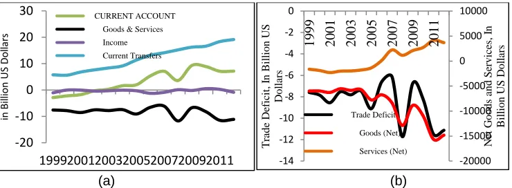
The Philippines is one of the world’s oldest open economies, which traded goods even prior to its discovery by the western world. Since 2004, the country has a positive Balance of Payment (BOP) position which is attributed to the current account surplus. This surplus was accounted to influx of current transfers and strong remittances of Oveseas Filipino Workers (income). Large trade deficit however, continuesly pulling this surplus (Figure 1.a) for more than a decades . The trade deficit in the country are attributed to large deficit in the traded goods (Figure 1.b).
In the aim of reducing huge gap between export and imports, the Philippine government passed Republic Act No. 7844, known as the "Export Development Act of
1994” to evolve export development into a national effort. This mandated the creation of Philippine Export Development Plan (PEDP) as export development strategy. The PEDP shall define the country's annual and medium-term export thrusts, strategies, programs and projects and shall be jointly implemented by the government, export and other concerned sectors.
(a) (b)
Figure 1. (a) Current account balance; (b) Trade Deficit (goods + services), Philippines, 1999-2012 Source of data: Philippine Institute of Development Studies (http://econdb.pids.gov.ph/tablelists/table/153)
Figure 2. PEDP export targets and actual exports, in Billion US Dollars Source: Targets are taken from PEDP while actual exports are taken from BSP
Figure 2 shows the PEDP targets versus the actual exports. In 2010, the PEDP export target for merchandise exports was 51 Billion USD, however, it only achieved 71% of the target. This leads the Philippines to target a forty percent (+40%) increase in export by 2013 and to exceed Philippine exports by one hundred twenty billion U.S dollars (US$ 120B) by 2016. The 2016 target is more than twice compared to the 2012 Philippine export value of US$ 57.5B (PEDP 2011-2013). In the actual target of PEDP for 2016, it only targeted 92 Billion USD lower compared to the planned target for 2016 mentioned in PEDP 2011- 2013. PEDP 2011-2013 only reached 65% of the target. This was achieved by building on the current business for the period 2011-2013 and developingKey Export Sectors that have high potential for growth. In the subsequent three years (2014-2016), growth will be attained by implementing an agro-industrial resource-base export development program. This target is in line with the changing characteristics of exports and global trade as the world recovers from the recent financial crisis and natural disasters in Japan, among others. The key features of these changes are the speedy growth of emerging economies with large consumer populations and the sluggish single-digit growth of developed markets. This will result in the re-balancing of consumption, export market size and supply chain configurations in relation to pre-crises periods
(PEDP, 2011-2013). These changes in global export environment pose opportunities for the Philippines to grow exports of merchandise and services. Achievement of this target requires understanding of the factors that prevent the Philippines to reach its export potential which both the institutional and infrastructures rigidities (behind the border) of the country or the rigidities of its trading partners (beyond the border). Several researches and efforts was conducted to understand and identify behind the border constraints on exports, however, it is surprising that there are very few, if any, in the literatures that focus on behind the border constraints (factors) of Philippine export. Understanding and reducing these rigidities may shrink trade deficits that will enhance and sustain positive current account position.
through the engagement process or even through unilateral reforms. It is of significant importance that each country may know its full potential with other countries or other regions in order to get the engagement process started. Enhancement of this trade flows will enhance welfare of people. This paper is focus on measuring efficiency and potential of the Philippines exports to its sixty-nine (69) trading partners. The measured efficiency and potential could be used as benchmark in expanding exports of the country through trade negotiations to potential markets.
Earlier studies have estimated the difference between observed values and the estimated predicted values by using an augmented gravity equation through Ordinary Least Squares (OLS) estimates as potential trade (Baldwin, 1994 and Nilsson, 2000) between a pair of countries. The OLS estimation procedure produces estimates that represent the centered values of the data set. However, potential trade refers to free trade with no restrictions to trade. Thus, for policy purposes, it is rational to define potential trade as a maximum possible trade that can occur between any two countries, which has liberalized trade restrictions the most, given the determinants of trade. This means that the estimation of the potential trade requires a procedure that represents the upper limits of the data and not the centered values of the data (Kalirajan, 2007). To address this, the concept of stochastic production frontier analysis which deals with the upper bound of the data set to measure the maximum possible output is utilized (Drysdale et al., 2000). This approach is known as the Stochastic Frontier Gravity Model.
This study analysed factors affecting trade of merchandise export. Merchandise exports was used as it accounts to 70% to 80% of the total exports of the country. It also aims to come up with technical efficiency estimates for each of the trading partner. Furthermore, the study assessed effectiveness of multilateral agreements of the Philippines on enhancing the volume of Philippine export. The factors considered in this study are “beyond the border” constraints and natural constraints to trade. This will also estimate export potential and compare it with actual export data to give an overview of export enhancing opportunities base on the frontier. Estimation of the model will follow the proposed method of Kalirajan and Finley (2005). The study includes comprehensive measures of “beyond the border” constraints which are product of recently established country specific indices which are not included in the studies in the literatures.
THE GRAVITY MODEL
The Gravity Model is based on the law of universal gravitation in physics developed by Isaac Newton in 1687 which described the gravitational force between two
masses in relation to the distance that lies between them (Newton, 1687), that is
𝐹𝑖𝑗 = 𝐺
𝑀𝑖𝑀𝑗
𝑑𝑖𝑗2 (1)
The gravitational force 𝐹𝑖𝑗 is proportional to the product
of the two masses 𝑀𝑖 and 𝑀𝑗 and inversely proportional
to the square of the distance 𝑑𝑖𝑗 that keeps the two
masses apart from each other. The gravitational constant G is an empirical determined value. This relationship is applicable to any context where the modeling of flows or movements is demanded (Starck, 2012).
The gravity equation was first applied to international trade flows by Timbergen in 1962. He assumed the relationship in equation 2.
𝑋𝑖𝑗 = 𝐴
𝑌𝑖𝛼𝑌𝑗 𝛽
𝐷𝑖𝑗𝛾 (2) There is a direct proportionality between the explanatory variables and the variable to be explained is not necessary implied. The exponents , and can therefore take values different from 1. These are elasticity of the exporting country’s GDP (), the elasticity of the importing country’s GDP () and the elasticity of distance (). By taking the natural logarithm of equation 2 and by adding the error term 𝜀𝑖𝑗 a linear relationship is
obtained (equation 3). This is traditionally estimated using the Ordinary Least Squares (OLS) regression analysis; the coefficients can be interpreted as elasticities.
log(𝑋𝑖𝑗) = log 𝐴 + 𝛼 log(𝑌𝑖) + 𝛽 log(𝑌𝑗) − 𝛾 log(𝐷𝑖𝑗)
+ 𝜀𝑖𝑗 (3)
Anderson (1979) was one of the first economists who developed a sound theoretical foundation of the gravity model that brought gravity model into mainstream economics. The development of the Anderson’s theoretical foundation of gravity model was gradual. His work became the basic theoretical framework for a gravity model of trade flows with the basic assumptions of homothetic preferences for trade goods across countries and using the constant elasticity of substitution (CES) preferences1. Anderson yielded the specification of aggregated trade flows as final gravity equation
𝑋𝑖𝑗 =
𝑌𝑖Φ𝑖Φ𝑗𝑌𝑗
∑ 𝑌𝑗 𝑗Φ𝑗
1 𝑓(𝑑𝑖𝑗)
[∑ 𝑌𝑗Φ𝑗 ∑𝑗Φ𝑗𝑌𝑗
1 𝑓(𝑑𝑖𝑗) 𝑗
]
−1
𝜀𝑖𝑗 (4)
where,
𝑋𝑖𝑗 = Exports of country 𝑖 to country 𝑗
Y= Income in country i and 𝑗
1See Starck, S. C. 2012. “The theoretical foundation of the Gravity Modelling:
𝑑𝑖𝑗= Distance between country 𝑖 and country 𝑗
Φ𝑖= The share of expenditure on all traded goods
and services in total expenditure of country Φ𝑖=
𝐹(𝑌𝑖𝑁𝑖), where Ni is the population in country 𝑖
Inherent Bias of the Gravity Model
According to Anderson (1979), the log linear of equation 4 resembles the standard gravity equation in equation 3, with an important difference. This difference is the bracket term in equation 4 which is:
[∑ 𝑌𝑗Φ𝑗 ∑𝑗Φ𝑗𝑌𝑗
1 𝑓(𝑑𝑖𝑗) 𝑗
]
−1
This is missing in the generally used empirical specification of the gravity model presented in equation 4. Anderson (1979) described this term as “the flow from 𝑖 to 𝑗 depends on economic distance from 𝑖 to 𝑗 relative to a trade weighted average of economic distance from 𝑖 to 𝑗 to all points in the system. Measuring the correct specification of the relative economic distance term is difficult because researchers do not know all the factors affecting this term. The economic distance can be affected by many factors, including institutional, regulatory, cultural and political, which are difficult to measure completely. These factors are referred to as ‘behind the border’ constraints of the importing countries or constraints to export.
Omission of this term in the empirical work of gravity model leads to the biasness of the estimation. This is because the term in the square brackets (economic distance term) of equation 4 affects the log-normal distribution of the error term. Therefore, the expected value of the error term is no longer zero (E(ij) ≠ 0) and the normality assumption of OLS is violated. This omission leads to heteroskedastic error terms and the log-linearization of the empirical model in the presence of heteroskedasticity leads to inconsistent estimates because the expected value of the logarithm of a random variable depends on higher-order moments of its distribution (Santos Silva and Tenreyro, 2003). Therefore, the OLS estimation on such gravity equations will be biased.
Aside from the violation of the OLS normality assumption, the estimation of these conventional gravity models through OLS provides the values at the mean of the observation or sample countries. This is problematic in determining trade potential which requires identifying the upper bound. To address these problems, the concept of stochastic production frontier analysis was incorporated to the gravity model. In this case, export potential is conceptually similar to a firm producing at the frontier. STOCHASTIC FRONTIER GRAVITY MODEL
The Gravity Stochastic Frontier Model is the Integration of Gravity Model and Stochastic Frontier Production Function Model which was formally introduced by Kalirajan (2000) to address the inherent bias of the conventional gravity model of trade and to estimate potential trade flows. With a stochastic frontier approach, the gravity equation can be written as:
𝑙𝑛𝑋𝑖𝑗𝑡= 𝑙𝑛𝑓(𝑌𝑖𝑗𝑡;)𝑒𝑥𝑝(𝑣𝑖𝑗𝑡−𝑢𝑖𝑗𝑡) (5)
where the term 𝑋𝑖𝑗𝑡 represents the actual exports from
country 𝑖 to country 𝑗. The term 𝑓(𝑌𝑖𝑗𝑡;) is a function of
the determinants of potential trade (𝑌𝑖𝑗𝑡) and is a vector
of unknown parameters. The single sided error term,
𝑢𝑖𝑗𝑡is the economic distance bias referred by Anderson
(1979), which is due to the influence of the “behind the border measures” of the importing country. This bias creates the difference between actual and potential trade between two countries. 𝑢𝑖𝑗𝑡takes value between 0 and 1
and it is usually assumed to follow a truncated (at 0) normal distribution, 𝑁(𝜇, 𝜎𝑢2). When 𝑢𝑖𝑗𝑡 takes the value
0, this indicates that the bias or country-specific “beyond the border constraints” are not important and the actual exports and potential exports are the same, assuming there are no statistical errors. When 𝑢𝑖𝑗𝑡 take the value
other than 0 (but less than or equal to 1), this indicates that the bias or country-specific “beyond the border” constraints are important and they constrain the actual exports from reaching potential exports. The double-sided error term 𝑣𝑖𝑗𝑡, which is usually assumed to be
𝑁(0, 𝜎𝑣2), captures the influence on trade flows of other
left out variables, including measurement error that are randomly distributed across observations in the sample. In this approach, it is assumed that the Philippines as an exporting country is very efficient (no significant behind the border constraints).
efficiency (TEX) of the economy) as the ratio of actual to potential exports as shown in equation 6.
𝑇𝐸𝑋𝑖𝑗𝑡=
𝑓(𝑌𝑖𝑗𝑡; 𝛽) exp(𝑣𝑖𝑗𝑡− 𝑢𝑖𝑗𝑡)
𝑓(𝑇; 𝛽)exp (𝑣𝑖𝑗𝑡)
= exp(−𝑢𝑖𝑗𝑡) (6)
The advantages of the suggested method of estimation of the gravity model are as follows: Firstly, it does not suffer from loss of estimation efficiency. Secondly, it corrects for the economic distance bias term, which is creating heteroskedasticity and non-normality, isolating it from the statistical error term. This isolation property will enable us to examine how effective are the importing countries “behind the border constraints” as major trade constraints. Thirdly, the suggested approach provides potential trade estimates that are closer to frictionless trade estimates. This is because the approach represents the upper limits of the data, which come from, those economies that have liberalized their trade restrictions the most (Miankhel, et al., 2009). Finally, the suggested method bears strong theoretical and trade policy implications towards finding ways of minimizing unilateral impacts to volume of trade.
DATA AND EMPIRICAL APPLICATION
Data Sources
This study utilized panel data consisting of 69 bilateral trading partners of the Philippines on merchandise exports from 2009 to 2012. The list of countries included in this study is shown in the appendix which was chosen based on their relative importance to Philippine merchandise exports. The aggregate data on merchandise export was taken from the Department of Trade and Industry (DTI). Data on Gross Domestic product as proxy to income and population as proxy for market size was taken from the World Bank. Data on bilateral distance (in kilometers), landlocked, language and land area was secured from the Centre d'Etudes Prospectivesetd' Informations Internationales (CEPII) which was developed by Mayer and Zignago (2005). “Behind the Border” variables of the importing partners including freedom from corruption (FC), fiscal freedom (FiscalF), business freedom (BF), labor freedom (LF), monetary freedom (MF), trade freedom (TF) investment freedom (IF) and financial freedom (FF) were taken from the Heritage Foundation. The list of APEC member countries was taken from apec.org while ASEAN member countries were taken from asean.org. World Trade Organization list of members was taken from wto.org.
Empirical Application
Adopting the methodology proposed by Drysdale et.al. (2000) and Kalirajan and Finley (2005), the stochastic
frontier approach of the gravity model in equation 5, imposing the variables proposed in this study can be rewritten as:
ln 𝑋𝑖𝑗𝑡= 𝛽0 + 𝛽1𝑙𝑛𝐺𝐷𝑃𝑗𝑡+ 𝛽2𝑙𝑛𝑃𝑜𝑝𝑗𝑡+ 𝛽3𝑙𝑛𝑑𝑖𝑠𝑡𝑖𝑗𝑡− 𝑢𝑖𝑗𝑡
+ 𝑣𝑖𝑗𝑡 (7)
where:
𝑋𝑖𝑗𝑡- is the total value of exports from Philippines (i) to
partner country (j) at time t.
𝐺𝐷𝑃𝑗- Gross Domestic Product of country j at time t as
proxy for income.
𝑃𝑜𝑝𝑗- population of country j as proxy for market size.
𝑑𝑖𝑠𝑡𝑖𝑗- is the geographical distance between the capital
cities of country i and j measured in kilometers.
𝑢𝑖𝑗𝑡 - Single sided error for the combined effects of
inherent economic distance bias or ‘beyond the border’ constraints, which is specific to the exporting country with respect to the particular importing country, creating the difference between actual and potential bilateral trade. 𝑢𝑖𝑗𝑡 is assumed to have an iid nonnegative half normal
distribution that is 𝑢𝑖𝑗𝑡~𝑖𝑖𝑑 𝑁(0, 𝜎𝑢2) 𝑣𝑖𝑗𝑡 – Double sided
error term that captures the impact of inadvertently omitted variables and measurement errors that are randomly distributed across observations in the sample. 𝑣𝑖𝑗𝑡 is assumed to follow an iid normal distribution with
mean zero and constant variance that is 𝑣𝑖𝑗𝑡 ~𝑖𝑖𝑑 𝑁(0, 𝜎𝑣2).
The disturbance term can be specified as: 𝜀𝑖𝑗𝑡= 𝑣𝑖𝑗𝑡−
𝑢𝑖𝑗𝑡
The inefficiency effect model is specified in equation 8 captures beyond the border constraints that contribute to Philippine merchandise export inefficiency.
𝑢𝑖𝑗𝑡= 𝛿0+ 𝛿1𝐴𝑃𝐸𝐶 + 𝛿2𝐴𝑆𝐸𝐴𝑁 + 𝛿3𝑊𝑇𝑂 + 𝛿4𝐿𝑎𝑛𝑔𝑗
+ 𝛿5𝐿𝑎𝑛𝑑𝑙𝑜𝑐𝑘𝑒𝑑 + 𝛿6𝐶𝐼𝑗+ 𝛿7𝑇𝐹𝑗+ 𝛿8𝐵𝐹𝑗
+ 𝛿9𝐼𝐹𝑗+ 𝛿10𝐹𝐶𝑗+ 𝛿11𝐹𝑖𝑠𝑐𝑎𝑙𝐹𝑗 + 𝛿12𝐿𝐹𝑗
+ 𝛿13𝑀𝐶𝑗+ 𝛿14𝐹𝐹𝑗+ 𝑤𝑖𝑗𝑡 (8)
where:
𝐴𝑃𝐸𝐶 - is a dummy variable that takes the value of 1 if country j is a member of Asia Pacific Economic Cooperation and 0, otherwise.
𝐴𝑆𝐸𝐴𝑁 - is a dummy variable that takes the value of 1 if country j is a member of Association of Southeast Nation and 0, otherwise.
𝑊𝑇𝑂- is a dummy variable that takes the value of 1 if country j is a member of World TradeOrganization and 0, otherwise.
𝐿𝑎𝑛𝑔𝑗- is a dummy variable, 1 if country js’ language is
English and 0 otherwise.
𝐿𝑎𝑛𝑑𝑙𝑜𝑐𝑘𝑒𝑑- is a dummy variable, 1 if the country j is landlocked and 0 otherwise.
𝐶𝐼𝑗- Cost of import goods of 20-foot container in US
𝑇𝐹𝑗- Trade Freedom index of country j, which is a
composite measure of the absence of tariff and non-tariff barriers in partner country j which includes quantity, price, regulatory, investment, customs restrictions and direct government intervention. The TF score of each partner country j is a number between 0 and 100. The higher the score implies lesser barriers of trade.
𝐵𝐹𝑗- is Business Freedom index developed by The
Heritage Foundation, is an overall indicator of the efficiency of government regulations of business. The BF scoreof each partner country j is a number between 0 and 100 with 100 as the freest business environment. 𝐼𝐹𝑗- Investment Freedom Index of partner country j
determines how free the flow of investment capital is. The higher the score, the freer is the investment into and out of specific activities, both internally and across the country’s border. The IF score of each partner country j is a number between 0 and 100 with 100 as the freest in terms of investment.
𝐹𝐶𝑗-Freedom from corruption index of country j developed
by Transparency International’s Corruption Perception Index (CPI).The FC score of each partner country j is a number between 0 and 100, the higher the score indicates little corruption.
𝐹𝑖𝑠𝑐𝑎𝑙𝐹𝑗- is Fiscal Freedom index of country j, is a
measure of the tax burden imposed by the government, it includes direct taxes on individuals and corporate incomes. The index lies between 0 to 100, the higher the index means the higher tax burden.
𝐿𝐹𝑗- Labor Freedom index of country j, measures various
aspect labor market’s legal and regulatory framework including minimum wages, laws inhibiting layoffs, severance of requirements and measurable regulatory restraints on hiring and hours worked.The index lies between 0 to 100, the higher the index means freer labor. 𝑀𝐹𝑗- Monetary Freedom index of country j, combines a
measure of price stability with an assessment of price controls. Both inflation and price controls distort market
activity. Price stability without microeconomic intervention is the ideal state for the free market. The index lies between 0 to 100, the higher the index means country j has a stable currency and market determined prices.
𝐹𝐹𝑗 –Financial Freedom index of country j, is a measure
of banking efficiency as well as a measure of independence from government control and interference in the financial sector. The index lies between 0 to 100, the higher the index means higher financial freedom.
The 𝑢𝑖𝑗𝑡 represents the measure of performance or, in
case of a production function, the degree to which actual output falls short of potential output given by the stochastic frontier equation. Thus, it represents “ineffeciency” of a country in its foreign trade arising from its lack of proper infrastructure or managerial expertise
(Kang, et.al,2006). An important assumption in this model is that the exporting environment in the home country does not impose any restrictions on home country’s exports. This model, while admitting that there are ‘behind the border constraints’ in home country, ignores these constraints and assumed to be randomly distributed across observations. In other words, the assumption is equivalent to saying that there are no significant ‘behind’ the border constraints for exports of home country.
The estimation of equations 7 and 8 was done simultaneously using Frontier 4.1 software of Tim Coelli (2004). Frontier follows the Kumbhakar and McGuckin (1991) and Reifschneider and Stevenson (1991) ideas to estimate all of the parameters in one step procedure to be consistent on the assumption that inefficiencies are independently and identically distributed.
RESULTS AND DISCUSSIONS
Philippine merchandise exports are dominated by manufactures. This is followed by machinery and transport equipment, office and telecom equipment, and integrated circuits and electronic components. Japan is the most important market which imports around 11% to 20% from 2007 to 2012. This is higher compared to the total exports of the Philippines to major regional trading blocs such as ASEAN, European Union (EU) and North America Free Trade Agreement (NAFTA). This is followed by China, Hong Kong, South Korea and Taiwan with 12%, 9%, 6% and 4% respectively in 2012.
*USA and Canada market share is 15.3%
Figure 3. Relationship of distance and value of Philippine merchandise exports, 2012. Sources of Data: CEPII and DTI
Table 1. Maximum likelihood estimates of the coefficients stochastic frontier gravity model for Philippine export among trading partners, 2009-2012.
Variable Est. Coefficient Std. err p-value
Constant 7.6039* 1.2498 0.0000
GDP 0.6971* 0.0489 0.0000
Population 0.2464* 0.0845 0.0039
Bilateral Distance -1.2193* 0.1121 0.0000
ns not significant at 5% level, * significant at 5% level
gravitational relationship on export flows are discussed in the next section.
Stochastic Frontier Estimates of the Gravity Model
Results of the simultaneous estimation of equations 8 and 9 were presented in Table 1 and 2. It shows that merchandise export flows from the Philippines to its trading partners are significantly affected by Income and population of the importing country, and the distance between them. These results are consistent with the literatures previously cited (Felipe et al., 2011; Naseret al., 2007; Amin, et al., 2009). Income of the importing country positively and significantly affects merchandise export flows of the Philippines at the 5% level of significance. The effect, however, is only minimal with income elasticity of 0.70%. Population a proxy to market size, revealed a positive relationship between Philippine exports and market size. On the average, 1% increase in the population or market size of the importing country, increases value of export from the Philippines by 0.25%.
On the other hand, bilateral distance was seen to have negative effect to export flows thereby reducing trade
between them. This variable is a proxy to transport costs and other cost of trade like communication cost, and transaction cost, among others. Thus, greater distance the higher the cost. That is, a percent increase in bilateral distance, decreases export flows by 1.21%. This estimate is relatively close to the estimated coefficients of distance by Kumar et al. (2010) which is -1.56% and Herera et al. (2011) which is -1.24%, among others. This implies that even with modern transport technology, distance/cost of trade in many forms still significantly affects trade flows among countries. For example, distance can reflect logistical difficulties. The study conducted by Djankov et al. (2006) revealed that each additional day taken to move the goods from warehouse to the ships reduces trade by at least 1%. This is equivalent to increasing the distance of a country from its trade partners by 70kms.These results suggest that to increase export flows of the country, it should focus on strengthening trade linkages/partnership in form of bilateral or multilateral agreement in nearby countries with fast growing population/ expanding markets and with higher income. This leads us to a very important question on “which nearby countries posed potentials for market expansion of Philippine export?”.
Australia Brazil
Canada
China Germany
Hong Kong
Japan S. Korea
Malaysia Netherlands
Singapore
Taiwan Thailand
USA
Vietnam
-5 0 5 10 15 20
Dis
tan
ce
in
th
o
u
san
d
k
ilo
m
eter
s
Market Share (70%) Market Share
(6.9%) Market Share
(23%) Market Share
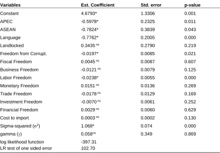
Table 2. Maximum likelihood estimates of coefficients of the inefficiency effect model for Philippine trade among trading partners, 2009-2012.
Variables Est. Coefficient Std. error p-value
Constant 4.6793* 1.3306 0.001
APEC -0.5978* 0.2325 0.011
ASEAN -0.7824* 0.3839 0.043
Language -0.7762* 0.2005 0.000
Landlocked 0.3435 ns 0.2790 0.219
Freedom from Corrupt. -0.0197* 0.0085 0.021
Fiscal Freedom 0.0045 ns 0.0087 0.607
Business Freedom -0.0121 ns 0.0079 0.125
Labor Freedom -0.0238* 0.0055 0.000
Monetary Freedom 0.0151 ns 0.0136 0.269
Trade Freedom -0.0178 ns 0.0129 0.169
Investment Freedom -0.0070 ns 0.0061 0.252
Financial Freedom 0.0029 ns 0.0060 0.629
Cost to import 0.0003 ns 0.0002 0.130
Sigma-squared (2) 1.068* 0.074 0.000
gamma () 0.058ns 0.349 0.869
log likelihood function -397.31
LR test of one sided error 102.70
*significant at the 5% level of significance,ns not significant at the 5% level of significance
The technical inefficiency effect model estimates are presented in Table 2. Trade agreements included in the analysis were APEC, ASEAN and WTO to capture the impact of international engagement/commitment entered into by the Philippine government. However, WTO was removed in the actual estimation to avoid double counting. If APEC and ASEAN turn out significant, will also imply that WTO is a significant variable. This is because WTO is the convergence of the members of ASEAN and APEC. Results revealed that the Philippines membership to APEC, ASEAN and WTO increases technical efficiency (negative sign of the coefficient indicates reduction of technical inefficiency) of the Philippine export flows to trading partners in almost the same degree. This implies the positive impact of Philippines active involvement to international trade negotiations in narrowing trade gap between trading partners.
The study also included trading partner’s “natural” specific characteristics such as language, and if the country is landlocked. Landlocked turns out insignificant at 5% level of significance, while common language significantly increases technical efficiency of export flows. This increases technical efficiency by 0.77%. This study
used the disaggregated components of economic freedom to capture the impact of country specific indicators covering macroeconomic stability, the role of the government and corporate sector in business, price stability, legal system and policies regarding investment and international trade. Among these indices only freedom from corruption and labor freedom significantly affects trade efficiency. This implies that less corruption in importing means freer flow, thus increasing technical efficiency of this flow. Corruption is a cost to trade. Freer labor which means less intervention of government in the labor market of importing country will also increase technical efficiency.
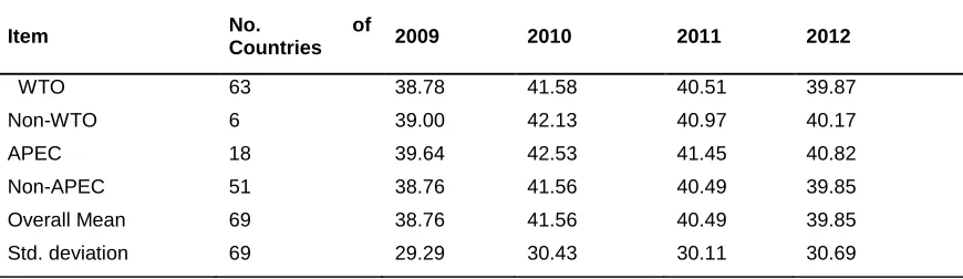
Table 3. Mean technical efficiency (in percent) of Philippine merchandise exports, by multilateral agreements, 2009-2012.
Item No. of
Countries 2009 2010 2011 2012
WTO 63 38.78 41.58 40.51 39.87
Non-WTO 6 39.00 42.13 40.97 40.17
APEC 18 39.64 42.53 41.45 40.82
Non-APEC 51 38.76 41.56 40.49 39.85
Overall Mean 69 38.76 41.56 40.49 39.85
Std. deviation 69 29.29 30.43 30.11 30.69
Export Performance
It covers Technical Efficiency (TE) of Philippine merchandise export flows to 69 markets in the world. TEs in four years period are changing minimally. The mean TEs for all sample ranged from 42 to 48% during these periods. Mean technical efficiency among the country groups in 2012 are relatively high, which is above the mean TE. Export flows is more efficient in NAFTA with TE of 73%, East Asia with TE of 72%, followed Members of APEC, ASEAN, EFTA and lastly EU with 69%, 62%, 50% and , 43% respectively.
Technical efficiency of merchandise exports to ASEAN member states is high, however relatively lower compared to TEs of NAFTA and countries in East Asia. This clearly implies that the Philippines is not taking full advantage of the benefits of regionalization through ASEAN. In this bloc, Singapore is the most efficient country which recorded 100% technical efficiency. This is followed by Malaysia (85%) and Thailand (78%). Cambodia and Indonesia recorded a very low technical efficiency. ASEAN as a natural bloc in Southeast Asian should further strengthen its trade facilitation among its member states given lower transport cost and existing agreements.
Trading partners in the East Asia (EA) recorded relatively high TEs. TE is high with Hong Kong, Japan and South Korea with 97%, 87%, and 81% in 2012 respectively. In this group, China recorded a very low TE of 23%. This implies that Philippines can further improve export to China and take advantage of its very large market for manufactured goods. This can be further facilitated through bilateral negotiations and further improve economic partnership. European Union, one of the major trading blocs of the world, is an important trading partner of the Philippines. Among the members of EU, United Kingdom (93%), and Denmark (93%) recorded the highest TE. Countries like Belgium, Finland, Netherlands, and Sweden also posted high TEs.
Currently, there is no existing trade agreement between the Philippines and EU or its member states except common involvement in WTO.
Among the trading blocs included in the study, NAFTA recorded the highest TE which is attributed to the high TEs of Canada and USA. Trading with this country deviates from the gravity concept, which then proved that trade can be improved through a very tight economic partnership. The relative export performance of the Philippines to countries with common agreements/cooperation and integration reveal that TEs of export flows between the Philippines to WTO and non-WTO countries almost did not differ. On the hand, Philippine export performance is relatively high in APEC member countries than to Non-APEC countries as shown in Table 3.
In general, the technical efficiency measure of export flow is quite low (38 to 42%), this suggests large deviations of actual observed export flows from the potential export flows estimated by the gravity equation. The standard deviation from the mean is 29-31% which means that the TEs are not that far from each other. The next section shows trade potential if countries in the sample operated at the frontier.
Export Potential
Figure 5. Plot of estimated potential export, by country, 2012
RECOMMENDATIONS
Given the result of the study, several insights/recommendations are suggested:
1)Philippine export sector is highly viable in increasing foreign reserve of the country. This is reflected in the very substantial export gap between estimated potential and observed actual outflow. To expand this outflow the country should intensify its engagement on bilateral and unilateral trade talks/agreements on countries within the region and target high- growth emerging markets.
2)Export inefficiency effect model reveals that Philippine membership to ASEAN is significant factor in reducing export inefficiency. This could lead to expansion of export flows within this “natural trade blocs” which has emerging demands and lower transportation cost. Technical efficiency estimates, however, of Philippine export outflow to ASEAN member states were not that high compared to technical efficiency of other trading blocs. This implies that the Philippines are not maximizing the benefits of this regionalization. The country must seek to comprehensively identify goods with comparative advantage relative to other members of the ASEAN. This will help the country maximize benefits of the 2015 ASEAN Integration. Furthermore, the country should increase efficiency of exportation by improving domestic infrastructure and strengthening the export sectors.
3)There should be unification, and strategic direction among players in the domestic export industries that will be supported by the government in terms of information monitoring and other support services. 4)In the international level, RTAs should move to stimulate/improve logistical services competition to
increase transportation efficiency and decrease cost of transportation and other cost.
5)Further study is needed, specifically, the inclusion of complementarity index, similarity index and other behind the border (domestic) factors in the gravity model.
REFERENCES
Amin RZ, Hamid, Saad N (2009). Economic Integration among ASEAN Countries: Evidence from Gravity Model. EADN Working pp. 40
Anderson JE (1979). A Theoretical Foundation for the Gravity Equation.American Economic Review.Santos Silva J.M.C. and S. Tenreyro, 2004.“The Log of Gravity”, FRB Boston Series, pp. 03-1.
Armstrong S (2008). Asian Trade Structures and Trade Potential: An initial analysis of South and East Asian Trade. Paper presented at the Conference on the Micro-Economic Foundation of Economic Policy Performance in Asia, 3-4 April, New Delhi.
Baldwin R (1994). Towards an integrated Europe. London: Centre for Economic Policy Research
Coelli TJ (1994). A Guide to FRONTIER Version 4.1: A Computer Program for Stochastic Frontier Production and Cost Function Estimation, Department of Econometrics, University of New England, Armidale, NSW, 2351 Australia
Djankov S, Freund C, Pham C (2006). Trading on Time. World Bank Policy Research Working Paper 3909.The World Bank, Washington, DC.
Pacific Press
Felipe J, Kumar U (2010). The Role of Trade Facilitation in Central Asia: A Gravity Model. Levy Economics Institute of Bard College, Working Paper.
Herrera EG, (2010). “Comparing Alternative Methods To Estimate Gravity Models of Bilateral Trade”, Department of Economic Theory, University of Granada.
Kalirajan K (2000). Indian Ocean Rim Association for Regional Cooperation (IORARC):Impact on Australia’s Trade”, J. Econ. Integr.,
Kalirajan K (2007). Regional Cooperation and Bilateral Trade Flows: An Empirical Measurement of Resistance, The International Trade Journal XXI: 85-107.
Kalirajan K, Findlay C (2005). Estimating Potential Trade Using Gravity Models: A Suggested Methodology, GRIPS-FASID Joint Graduate Programme, Tokyo,Japan.
Kalirajan KP, Shand RT (1999). Frontier Production Functions and Technical Efficiency Measures, Journal of Economic Surveys 13(2), Blackwell Publishers. Kumar U, Felipe J (2010). The Role of Trade Facilitation
in Central Asia: A Gravity Model, pp. 628,
Miankel AK, Thangavelu S, Kalirajan K, (2009). On Modeling and Measuring Potential Trade, Quantitative Approaches to Public Policy Conference in Honor of Professor Krishna Kumar, Bangalore, August 9-12 Naser, S. and K. Kalirajan (2007). Export Performance of
South and East Asia in Modern Services, ASARC.
Newton I (1687). Philosophiænaturalis principia mathematica, retrieved 5 August 2013 from University of Cambridge – Cambridge Digital Library:
http://cudl.lib.cam.ac.uk/view/PR-ADV-B-00039-00001/9.
Nilsson L (2000). Trade Integration and the EU Economic Membership Criteria, Eur. J. Pol. Econ., 16: 807–827.
Starck SC (2012). The theoretical foundation of the Gravity Modelling: What are the developments that have brought gravity modeling into mainstream economics?,A Master Thesis, Department of Economics, Copenhagen Business School.
Tinbergen J (1962). Shaping the World Economy: Suggestions for an International Economic Policy, The Twentieth Century Fund, New York.
Accepted 28 June, 2014.
Citation: Deluna RS, Cruz ED (2014). Philippine Export Efficiency and Potential: An Application of Stochastic Frontier Gravity Model. World Journal of Economic and Finance. 1(2): 006-015.
Copyright: © 2014 Deluna and Cruz. This is an open-access article distributed under the terms of the Creative Commons Attribution License, which permits unrestricted use, distribution, and reproduction in any medium, provided the original author and source are cited.
Appendix 1. Trade partners of Philippine merchandise exports included in the study.