Download Download PDF

(1)

INFLUENCE OF SOME VARIABLE PARAMETERS ON

HORIZONTAL ELLIPTIC MICRO-CHANNELS

WITH INTERNAL LONGITUDINAL FINS

I. K. Adegun1*_{, T. S. Jolayemi}2_{, O. O. Olayemi}3_{, O. T. Popoola}4

1,3,4_D_{EPARTMENT OF}_M_ECHANICAL_E_NGINEERING_,_F_{ACULTY OF}_E_{NGINEERING AND}_T_ECHNOLOGY_,_U_NIVERSITY

OF ILORIN,ILORIN,NIGERIA

2_D_{EPARTMENT OF}_M_ECHANICAL_E_NGINEERING_,_I_{NSTITUTE OF}_T_ECHNOLOGY_,_K_WARA_S_TATE_P_OLYTECHNIC_, ILORIN,NIGERIA

E-mails: 1_{[email protected]}_,2_{[email protected]}_,

Abstract

The study investigates the laminar flow and heat transfer characteristics in elliptic micro-channels of varying axis ratios and with internal longitudinal fins, operating in a region that is hydrodynamically and thermally fully developed; purposely to determine the effects of some salient fluid and geometry parameters such as Reynolds number, Prandtl number, aspect ratio ( and fin heights on flow pattern and rate of heat transfer. Numerical method using the finite difference technique was adopted for the solution. A code in Quick Basic was developed to generate the results. Results show that fin height of H=0.6 provided the optimum heat transfer enhancement for the configuration of e = 0, e= 0.433 and e=0.714; for e=0.866, fin height of H= 0.4 is tolerable. Result also show that Nusselt number increases with Reynolds number for all axis ratios investigated. However, at Re=200 a slight trough was observed in Nusselt number Versus Reynolds number relationship indicating a critical flow condition. It was also established that atPr≥5, Nusselt number and bulk fluid temperature, are independent of fluid properties.

Keywords: Ellipse, Micro-channels, internal fins, Heat transfer, Fluid flow

Nomenclature a Major axis, m

A Cross-sectional area, m2 b Minor axis, m

Fluid specific heat, kJ/ kg k Hydraulic diameter,

, e Eccentricity; √1 F Number of fins H Normalized fin height k Iteration counter

Thermal conductivity of fluid w/mK Thermal conductivity of wall w/mK n exponent in hyperellise formula. Mean Nusselt number equ. (21) p Pressure, N/m2

Pe Peclet number Pr Prandtl number

r Dimensional equivalent radius of the elliptic geometry.

Dimensional radius along the Azimuthal direction

Non-dimensional equivalent radius of the elliptic geometry

Re Reynolds number

T Dimensionless temperature

b

T Bulk fluid temperature W Dimensionless wall thickness

(

r

,

φ

,

x

)

Modified cylindrical coordinate

x

Axial direction

∂ Partial differential

w

T Wall temperature U Dimensionless velocity

(2)

NIGERIAN JOURNAL OF TECHNOLOGY VOL.32,NO.2,JULY 2013

351

Greek symbols

c

Γ Perimeter

∈ or AR Axis ratio = a b

Non-dimensional coordinate =_! " Viscosity, N.S/m2

# Angle of channel inclinations $ Azimuthal direction

% Fluid density, kg/m3

& Fin half angle& = ', finned sectors 3 Unfinned sector

4 Limits

Subscripts b Bulk m mean w Wall

1. Introduction

The need for the efficient removal of internally generated heat in micro-electronic components, coupled with the growth of micro fluidic-systems, arising from their promise for potential incorporation in a wide variety of unique, compact and efficient cooling applications such as micro-electronic cooling, fuel cell technology, micro-reactors, medical and biomedical devices, has motivated many researchers to investigate microscale transport phenomena. These micro heat exchangers or heat sinks have specific characteristics such as extremely high heat transfer surface area per unit volume, high heat transfer coefficients and low thermal resistance [1-6]. The laminar flow with forced convective mechanism through ducts with different geometries was studied by many researchers analytically, numerically, and experimentally; thereby making this type of study to be very vital in challenging research activities in the field of heat transfer. Foong el al [7] studied the three dimensional laminar convective heat transfer in microchannels with longitudinal fins. They presented the results of average Nusselt number as function of fin height ratio which identified a maximum fin height. In the case of normal-size channel or duct, Hassan and Siren [8] investigated and found that for a heat exchanger constructed from tubes of elliptic cross-section with the major axis

parallel to the air flow, the air pressure drop is low due to its smaller frontal area. The lower pressure results into decrease in pumping power required by the fan, which is the main source of energy consumption in an air cooled heat exchanger. The concept of microchannel heat sinks was first demonstrated by Tuckerman and Peace in 1981[1]. Their pioneering work has been a remarkable breakthrough in the use of micro-channels for high heat flux dissipation devices. In the area of heat transfer enhancement techniques in micro-channels, Stunke and Kandlikar [9] reviewed and summarized the single-phase heat transfer enhancement techniques used in micro-channel and mini-micro-channel flows. They presented a list of passive and active thermal enhancement techniques. Palm [10], estimated that the use of micro-channel heat sinks will increase significantly within the next few years owing to its recognized cooling potential. Micro-channel experiment studies conducted by Pfahler etal [11,12], Harley et al [13], Choi et al,[14], Stanley [15] and Gao et al [16, 17] confirmed that the continuum theory holds in micron size channels. It was found from the Numerical study conducted by Shakuntala [18] involving CFD analysis of forced convection cooling of electronic chips. He asserted that the validation of the use of commercial codes for the generation of numerical results for fluid flow in micro-channel is an ongoing process. Based on this, the current authors had tried to develop their own codes for the generation of results using Qb-45.

However, it was also discovered from the literature that many researchers that worked in this area had not considered critically the use of fins in micro-channels of elliptic geometry. In this investigation the governing equations were solved using finite difference method because of its simplicity and ease of convergence.

2. Methodology

(3)

352

difference scheme, finite element and finite volumes.

However, the finite difference technique with symmetrical boundary condition was adopted for the present model because of its simplicity and stability. The symmetry boundary condition reduces the computational time and iteration for convergence.

The physical model adopted for this study is a horizontal microchannels of elliptic geometry with internal longitudinal fins in modified cylindrical co-ordinate system

(

r

,

φ

,

x

)

. The microchannel and all the internal longitudinal fins are shown in the schematic diagram of Fig. 1 The fins form an integral part of the

micro materials and are of trapezoidal cross-section. The specific boundary conditions for the channel at the symmetrical wall with all relevant parameters considered in the domain are all included in the model. The temperature of the fluid at inlet is assumed uniform while neglecting the axial heat fluxes in the duct and fluid. Internal longitudinal fins are arranged symmetrically along the axis inside the channel. The flow is laminar with forced convective mechanism and thermal boundary condition of constant heat flux at the outer wall of the finned channel is assumed.

Fig. 1 (a): Horizontal Microchannel of elliptic cross-section with internal longitudinal fins.

Fig: 1(b): Computational Domain and applicable boundary conditions of the elliptic geometry.

Axis of symmetry

5 5

R=

∆5

$

Solid Region Wall

Fins

Fluid Region

i

w

∝

3

'

R S

T

G _Z

Q

0

a

N O

A B C D E

F

w

j

b

P S

M

M H

(4)

353

It is assumed to be a steady state incompressible fluid flow and the velocity profile is fully developed in the channel. There is only one non-zero velocity component which is in the flow direction, vx. Thus

ν

_r

=

ν

_φ

≅

0 ,

ν

_r

,

ν

_φ are insignificant

when compared with

ν

_r

. The effect of gravity is neglected except in the axial direction and assumption of no-slip condition at the walls are considered.

2.2 Governing Equations

Based on the assumption made, the Navier- stokes equations are reduced to the following governing equations:

2.2.1 Continuity equation

0

1 =

∂

+

∂

+

∂

x

U

r

U

r

U

_r _r _x

φ

(1)

2.2.2 Momentum Transport Equations.

Since pressure varies only on the axial direction, the momentum transport equation for the geometry reduces to:

µ

θ

ρ

µ

ϕ

sin

1

2 2 2 2 2

g

x

p

r

U

r

U

r

U

_r

+

∂

=

∂

+

∂

+

∂

(2) Where

ρ

g

x

(

ρ

g

sin

θ

)

denotes the body force term as a result of channel inclination.

2.2.3 Energy Transport Equation

The energy transport equation for a steady flow in the absence of viscous dissipation term

φ

_ω

is

          ∂ ∂ = ∂ ∂ + ∂ ∂ + ∂ ∂ region solids other and fins for region fluid for x t U t r r t r r t x ... 0 ... ... 1 1 2 2 2 2 2

α

ϕ

(3)

2.3. Boundary conditions

Considering the assumptions, the boundary conditions for equation (2) are:

0 =

∂

φ

x

U













−

≤

+

=

−

≤

=

)

0 (

;

)

0 (

;

0 h

r

h

r

φ φ

β

α

φ

(4)         − ≤ ≤ + + = − ≤ ≤ = = ∂ ∂ ) 0 ( ; ) 0 ( ; 0 @ 0 2 2 h r r r h r r U_x φ φ

β

α

φ

(5) For interface between solid and fluid. No-slip condition: = 0

                  − = + + ≤ ≤ + ≤ ≤ − + = ≤ + ≤ ≤ ≤ ≤ − = − = ≤ ≤ = h r r r r r h r r r r r h r h r r U φ φ φ φ φ φ φ β α φ β α β α φ β α φ α α φ α φ ); ( ) ( ; ; ; ; 0 @ 0 (6) Similarly, boundary condition for energy transport equation (3) is;

For Fluid region (symmetry condition)













−

≤

+

=

−

≤

=

∂

h

r

h

r

t

_f φ φ

β

α

φ

;

0

0 ;

0 @

0

(7) For Solid region (symmetry condition)













+

≤

−

+

=

+

≤

−

=

∂

w

r

h

r

w

r

h

r

t

_s φ φ φ φ

β

α

φ

;

0 @

0

(8) For outer wall of the channel

w r r w r

t

ks

q

+ = +

∂

−

φ φ

φ

(9)

for Interface between solid and fluid

                  − = + + ≤ ≤ + ≤ ≤ − + = ≤ + ≤ ≤ ≤ ≤ − = − = ≤ ≤ = h r r r r r h r r r r r h r h r r t ts s

φ φ φ φ φ φ φ β α φ β α β α φ β α φ α α φ α φ ); ( ) ( ; ; ; ; 0 @ (10) 2.4 Normalization parameters

The governing equations and associated boundary conditions are non-dimensionalized by the following transformation parameters:

,

a

w

W

a

h

H

a

r

ap

x

X

e

=

η

φ

a

b

e

= 1−(∈)2, ∈= ,

φ

η

₂ ₂

(5)

354

a

r

R

= ,

k

C

k

K

_p f

s

₌

µ

=

,

Pr

* , t

a

U

Pe

a

U

_max

2

_max

,

2 Re

=

µ

ρ

f h h k qa t t T a d D adx dp g Pk 0 , , = = −

=

ρ

,

      ∂ ∂ − = x p a u U

µ

2 max )

( [19, 20, 21, 22 and 23]

2.4.1 Normalized Momentum Transport Equation

θ

φ

1 Re

Pr

sin

1

2 2 2 2 2

−

=

∂

+

∂

+

∂

U

R

U

R

U

(11) Normalized Boundary Condition for Eq (11): For symmetry condition













− ≤ ≤ + + − ≤ ≤ = = ∂ ∂ H R r H R U 1 0 ; 0 ; 0 @ 0 2 2

β

α

η

φ

(12) For interface between solid and fluid

                − = + + ≤ ≤ + ≤ ≤ − + = ≤ + ≤ ≤ ≤ ≤ − = − = ≤ ≤ = H R r R H R R H H R U 1 ; ; ; ; ; 0 @ 0 β α φ β α η η β α φ η β α φ α η η α φ η α φ (13)

2.4.2 Normalized Energy Transport Equation

        ∂ ∂ = ∂ ∂ + ∂ ∂ + ∂ ∂ fin and channel for fluid for X T U T R R T R R T 0 2 1 1 2 2 2 2 2

φ

(14)

2.4.3 Normalized Boundary Condition for equation (14)

For fluid region (Symmetry condition)













−

≤

+

=

−

≤

=

∂

H

R

H

R

T

_f

1

0 ;

0 @

0 γ

β

α

φ

η

φ

(15)

For Solid region (Symmetry condition)













+

≤

−

+

=

+

≤

−

=

∂

W

R

H

W

R

H

T

_s

1

1 ;

;

0 @

0 γ

β

α

φ

η

φ

(16)

For outer Wall of the Channel

*

1 k

R

T

w R

−

=

∂

+ =η (17)

For Interface between solid and fluid

                − = + + ≤ ≤ + ≤ ≤ − + = ≤ + ≤ ≤ ≤ ≤ − = − = ≤ ≤ = H R R H R R H H R T Tf s

1 ; ; ; ; ; 0 @ γ β α φ β α η η β α φ η β α φ α η η α φ η α φ (18)

3. Solution techniques and computational procedure

3.1 Solution Technique

The governing equations with its associated boundary conditions were solved numerically employing the Gauss-Seidel iteration technique subjected to some boundary constraints. For the discretisation of the governing equations, the central differences were used for the second-order derivatives, and the forward and backward differences were used for the first-order derivatives. Algebraic equations obtained for each variable were solved by simple form of Gauss-Seidel iterative procedure.

Convergence of the iteration procedures for the governing equations were achieved when the following criterion were satisfied. [24]

ε

≤       ₋ + ik ik ik u B u B u B ) ( ) ( ) ( max 1 (19)

Where B(u) represents the variable U or T, k is the iteration counter and

ε

=

10

−6

Consequently, the Nusselt number, surface heat transfer coefficients were obtained from the numerical simulation once the convergence criterion was satisfied.

3.2 Computational Procedure

(6)

355

energy transport equation for the fluid and solid region. A non-uniform grid pattern of 26x20 points was employed for the micro-channel geometries with axis ratios 0.25, 0.33, 0.5, 0.8 and 1. All successive calculations of the present study are based on these grid sizes. To ensure the accuracy of the numerical result, numerical tests were carried out with different grid sizes to determine the effect of grid size in the numerical results, before arriving at an appropriate mesh size.

Computed values for Nusselt number, average velocity, bulk fluid temperature were evaluated by varying the parameters of interest, such as, Reynolds number, Prandtl number, fin height and aspect ratios, to determine their effects on fluid flow and heat transfer.

3.3 Evaluation of the Mean Nusselt Number Nusselt number represents the rate of heat transfer across the wall. The tendency of fins in providing heat transfer augmentation is critically analyzed by values of Nusselt number.

Nusselt Number

f h m

k

D

x

h

Nu

)

(

)

(

=

[23]

(20)

Hence, Nusselt number is given by:

1

)

(

≤

−

∂

R h b w

D

T

R

T

(21)

Where D_h represents the hydraulic diameter of the elliptic micro-channel.

The hydraulic diameter (D_h) for internally finned longitudinal ellipse is derived as

  



+ − +

+

  

 −

− =

) sin ( ) ( 360 ) (

180 ) 2 ( 4

a H H R Fa b a

H R FHa ab Dh

π π

(22)

4. Results and discussion 4.1 Program Validation

The program for implementing the scheme was written in Qb-45 a version of Basic programming language. In order to validate the modeled scheme, the unfinned convectional duct results from Javery [25] and Sakalis et al [26] were compared with a case of unfinned channel modeled in the present study. The comparison is shown in Fig. 2 where the variation of mean Nusselt number as a function of aspect ratio is presented. As can be seen from Fig. 2, the Nusselt number of the microchannel is a bit higher than that of the convectional duct. This is in line with what shakuntala [18] observed in his research work. Having completed the grid independence study, and validation of the modelled scheme by comparison with result available in literature, the results for the finned micro-channel are given in Figs. 3-13.

4 4.1 4.2 4.3 4.4 4.5 4.6 4.7 4.8 4.9 5

0.25 0.5 1

N

u

ss

e

lt

n

u

m

b

e

r

Aspect ratio

Present study (V. Javery) (V.D Sakalis et al)

(7)

356

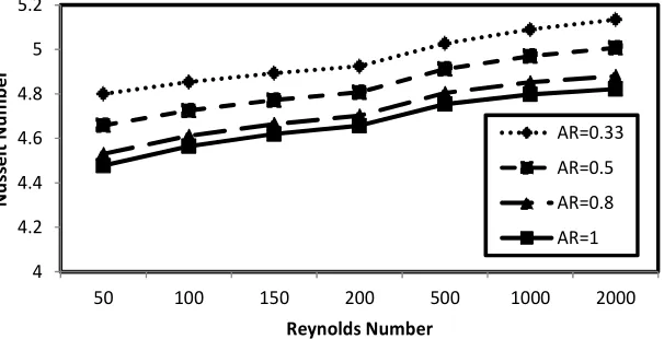
Fig. 3 shows the plot of mean Nusselt number as a function of Reynolds number flow regimes for different axis ratios. As can be seen from the figure, the larger the aspect ratio the lesser the mean Nusselt number. It is also worthy note that at R=200 for all the geometries investigated, the plot formed a slight trough indicating a critical flow condition.

Figs. 4 represent the Variation of mean Nusselt number as a function of aspect ratio for various Reynolds numbers. From the figure, Nusselt number attained highest value at the lowest aspect ratio.

Figs 5 and 6 depict the plot of mean Nusselt number versus Fin height for e = 0 and e = 0.433 respectively. Fig. 5 shows that the mean Nusselt number increases significantly as the fin height increases in the range0≤H ≤0.6. At 0.6≤H ≤0.9 Nusselt number also increase with Fin Height but at a lower rate.

This interesting observation at H =0.6 shows that fins are used to enhance the rate of heat transfer and increasing the fin height beyond the optimum fin height of H =0.6 may grossly affect fluid flow and could impede the rate of heat transfer by the equipment.

Similarly Fig. 6 shows that the heat transfer equipment will give an optimum performance at H =0.6 as Nusselt Number increases steadily with fin height in the range of

6 . 0

0≤H ≤ While at 0.6≤H ≤0.8 there is obvious drop in the rate at which Nusselt number increases with fin height. Hence, it is shown from both Figs. 5 and 6 that the optimum performance of heat transfer equipment is achieved when fins are used within the range of 0≤H ≤0.6 and there exist an optimum fin height of H =0.6 that gives the best rate of heat transfer.

4 4.2 4.4 4.6 4.8 5 5.2

50 100 150 200 500 1000 2000

N

u

ss

e

lt

N

u

m

b

e

r

Reynolds Number

AR=0.33

AR=0.5

AR=0.8

AR=1

Fig. 3. Variation of mean Nusselt number as a function of Reynolds number flow regimes for various aspect ratio . For H=0.2, Pr=0.7, F=4, α=3º, W=0.2.

4.2 4.3 4.4 4.5 4.6 4.7 4.8 4.9 5 5.1 5.2

0.33 0.5 0.8 1

N

u

ss

e

lt

N

u

m

b

e

r

Aspect Ratio Re=100

Re=500 Re=2000

(8)

357

4.552 4.554 4.556 4.558 4.56 4.562 4.564 4.566 4.568 4.57 4.572 4.574

0 0.2 0.4 0.6 0.7 0.8 0.9

N

u

ss

e

lt

N

u

m

b

e

r

Fin Height

e=0

Fig. 5. Variation of Mean Nusselt Number as a function of Fin height. For e=0, Pr=0.7, F=4, α=3º, W=0.2

4.576 4.578 4.58 4.582 4.584 4.586 4.588 4.59 4.592 4.594

0 0.2 0.4 0.6 0.7 0.8

N

u

ss

e

lt

N

u

m

b

e

r

Fin Height

e = 0.43

Fig. 6. Variation of mean Nusselt number as a function of Fin height. For e=0.433, Pr=0.7, F=4, α=3º, W=0.2

Figs 7 and 8 represent the variation of mean Nusselt number as a function of Fin height for

714 . 0

=

e and e=0.8666 respectively. Both Figs 7 and 8, shows similar response of Nusselt number with fin height as increasing fin height results to increasing values of Nusselt number.

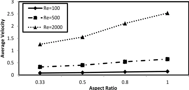
Fig. 9 shows the variation of average velocity with aspect ratio for different Reynolds number flow regimes. It can be seen that, as the aspect ratio increases the average velocity increases, for all Reynolds number investigated. Fig 10 depicts the variation of the average velocity with the fin height at eccentricity e=0. The plot shows that the higher the fin height, the lower the average velocity.

(9)

358

Nusselt number increases with Prandtl number in the range0.7≤Pr≤5 in all the axis ratios investigated. It is evident from the plot that at P ≥ 5, regardless of the axis

ratios, the rate of increase in Nusselt number to Prandtl number is nearly constant. At this point, Nusselt number is independent of the property of the fluid.

4.634 4.635 4.636 4.637 4.638 4.639 4.64 4.641 4.642 4.643 4.644 4.645

0 0.2 0.3 0.4 0.5 0.6

N

u

ss

e

lt

N

u

m

b

e

r

Fin Height

e = 0.714

4.721 4.7215 4.722 4.7225 4.723 4.7235 4.724 4.7245 4.725 4.7255 4.726 4.7265

0 0.1 0.2 0.3 0.4

N

u

ss

e

lt

N

u

m

b

e

r

Fin Height

e = 0.866

0 0.5 1 1.5 2 2.5 3

0.33 0.5 0.8 1

A

v

e

ra

g

e

V

e

lo

c

it

y

Aspect Ratio Re=100

Re=500

Re=2000

(10)

359

0 0.02 0.04 0.06 0.08 0.1 0.12 0.14 0.16 0.18 0.2

0 0.2 0.4 0.6 0.7 0.8 0.9

A

v

e

ra

g

e

V

e

lo

c

it

y

Fin Height

e = 0

Fig. 10 Variation of average velocity with fin height . For e= 0, H=0.2, F=4, α=3º, W=0.2

0 0.02 0.04 0.06 0.08 0.1 0.12 0.14 0.16 0.18 0.2

0.33 0.5 0.8 1

B

u

lk

F

lu

id

T

e

m

p

e

ra

tu

re

Aspect Ratio

Re=100

Re=500

Fig. 11: Variation of bulk fluid temperature with aspect ratio for different Reynolds number flow regimes. For H=0.2, Pr=0.7, F=4, α=3º, W=0.2

0 0.02 0.04 0.06 0.08 0.1 0.12 0.14 0.16 0.18 0.2

50 100 150 200 500 1000 2000

B

u

lk

F

lu

id

T

e

m

p

e

ra

tu

re

Reynolds Number

AR=0.33

AR=0.5

AR=0.8

AR=1

(11)

360

4.3

4.4 4.5 4.6 4.7 4.8 4.9 5 5.1

0.7 1 2 5 6 7 8 9

N

u

ss

e

l

N

u

m

b

e

r

Prandtl Number

AR=0.5 AR=0.8 AR=1

Fig. 13. Variation of Nusselt number with Prandlt Number for different aspect ratios. For H= 0.2, F = 4, α = 30_{, W = 0.2}

0 0.02 0.04 0.06 0.08 0.1 0.12 0.14 0.16 0.18 0.2

0.7 1 2 5 6 7 8 9

B

u

lk

F

lu

id

T

e

m

p

e

ra

tu

re

Prandtl Number

AR=0.5 AR=0.8 AR=1

Fig. 14. Variation of Bulk fluid temperature with Prandlt number for different aspect ratios. For H= 0.2, F = 4, α = 30_{, W = 0.2}

Fig. 14 shows the variation of bulk fluid temperature against Prandtl number for different axis ratio. This is similar to the trend of Fig. 13 as bulk fluid temperature increases with Prandtl number in the range

5 Pr 7 .

0 ≤ ≤ for all axis ratio considered. While at P ≥ 5, regardless of the axis ratios, the rate of increase in Bulk fluid temperature to Prandtl number is nearly constant. At this point, Bulk fluid temperature is independent of the property of the fluid.

5. Conclusions

Based on the numerical study conducted on the horizontal elliptic micro-channel with internal longitudinal fins, and within the range of Reynolds numbers examined which varied from 50 to 2000. It can be concluded that the internal fins in micro-channels have

the tendency to augment the rate of heat transfer.

(12)

361

increases from 0.33 to 1 the mean Nusselt number decreases while the average velocity and the bulk fluid temperature increases. For fluid of Prandtl number ≥ 5, Nusselt number and bulk fluid temperature were independent of the fluid’s properties and therefore solely depend on the eccentricity and aspect ratio of the geometry .

6. References

[1] Tuckerman, D.B. and Pease, R.F. “High

performance heating sinking for VLSI”, IEEE

Electron device letters, Vol.5, 1981, pp. 126-129.

[2] Ho, C.M. and Tai, Y.C. “Micro-Electro-

Mechanical-Systems (MEMS) and Fluid

Flows”, Annual Review of Fluid Mechanics,

Vol. 30, 1998, pp. 579-612.

[3] Cha, S.W., Hayre, R.O. and Prinz, F.B. “The

influence of size scale the performance of

fuel cells” Solid State Ionics, Vol. 175, 2004,

pp. 789-795.

[4] Gunther, A. I., Khan, S. A., Thalmann, M.,

Trachsel, F .and Jensen, K.F, “Transport and reaction in micro scale segmented gas-liquid

flow” lab on a chip, Vol.4, 2004, pp. 278-286.

[5] Efenhauser, C., Manz, A., and Dinor, M.W.

“Glass chips for high-speed capillary

electrophoresis separation with

submicrometer plate heights”, Analytical

Chemistry, Vol. 65, 1993, pp. 2637 – 2642.

[6] Yang, C.,Wu, J., Chien, H.,and Lu, S., “Friction

characteristics of water, r-134a, and air in

small tubes”, MicroscaleThermophysical

Engineering, Vol. 7,2003,pp 335-348.

[7] Foong, J.L.A., Ramesh, N., Chandratilleke, T.T.

“Laminar convective heat transfer in a microchannel with internal longitudinal fins”

International Journal of Thermal Science, Vol. 48, 2009, pp. 1908-1913

[8] Hassan, A. and Siren, K. “Performance

investigation of plan and finned tube

evaporatively cooled heat exchanger” Applied

Thermal Engineering, Vol. 23, Number 3, 2004, pp. 325-340.

[9] Steinke, M.E., and Kandlikar, S.G.

“Usage-phase Liquid Friction factors in

microchannels,” International Journal of

Thermal Science, Vol. 45, 2006, pp. 1073 – 1083.

[10] Palm, B. “Heat Transfer in Microchannels”

Microscale Thermophysical Eng. Vol.5, Number 3,2001, pp. 155 – 175.

[11] Pfahler, J., Harley, J., Bau, H., and Zemel, J.N.

”Liquid transport in Micron and Submicron

Channels” sensors and Actuators, Vol.

A21-A23,1991,pp 431-437.

[12] Pfahler, J., Harley, J., Bau, H., and Zemel, J.N.

“Gas and liquid transport in small

Channels”ASME Micromechanical Sensors

Actuators Systems, Vol. 32, 1991, pp.49-58.

[13] Harley, J.C., Huang, Y., Bau, H., Zemel, J.N. “Gas

flow in Microchannels” Journal of Fluid

Mechanics, Vol. 284,1995,pp. 257-274

[14] Choi, S.B., Barron, R.F. and Warrington, R.O.

“Fluid flow and Heat Transfer in micro

tubes”, ASWE Micromechanical sensors,

Actuators and Systems, Vol. 32, 1991, pp. 123-124.

[15] Stanley, R.S. “Two-phase Flow in

Microchannels” PhD Thesis, Louisiana Tech.

University ,1977

[16] Gao, P., Person, S. L. and Marinet, M. F. “Scale

Effect on Hydrodynamics and Heat Transfer in Two Dimensional Mini and Microchannel”

International journal of Thermal Science. Vol. 41, 2002, pp. 1017-1027.

[17] Cao, B. Chen, G. W. and Yuan, Q. “Fully

Developed Laminar Flow and Heat Transfer

in Smooth Trapezoidal Microchannel”

International Communication Heat and Mass Transfer, Vol. 32, 2005, pp. 1211-1220.

[18] Shakuntala Ojha, “ CFD Analysis on Forced

Convection Cooling of Electronic Chips” A

Masters Thesis, Department of Mechanical

Engineering, National Institute of

Technology, Rourkela, 2009.

[19] Tamayol, A., and Bahrami, M. “Analytical

Solutions for Laminar Fully-developed Flow in Microchannel with Non-Circular

Cross-Section” ASME Fluids Engineering Division

Summer meeting August 2-5, 2009, Vail, Colorado USA.

[20] Bello-Ochende, F. L., Adegun, I. K.,“Scale

Analysis of Laminar forced Convection within the Entrance of Heated Regular

Polygonal Tubes” Journal of Mathematical

Association of Nigeria (ABACUS), Vol. 31, Number 2A, 2004,pp 28-41.

[21] Necatic, O. Boundary Value Problems of heat

Conduction international Textbook company Pennsylvania pp. 395-416.

[22] Yoav Peles, Internal Forced convection,

(13)

362

[23] Marinet, M.F. and Tardu, S. “Convective Heat

Transfer” Solved Problems, www.wiley.com,

Accessed on June 12,2012.

[24] Holman, J. P. “Heat Transfer” Tata

McGraw-Hill Edition, Eighth SI Metric Edition, 2002, pp. 101-120.

[25] Javery, V. “Analysis of Laminar Thermal

Entrance region of Elliptical and Rectangular

channels with Kantorowish Method”

Warme-und Stoffubertragung. Vol.9, 1976, pp. 85-98.

[26] Sakalis, V. D., Hatzikonstantinou, P.M.

KafouSias, N. “Thermally developed flow in elliptic ducts with axially variable wall temperature flow in elliptic ducts with

axially variable wall temperature

distribution” International Journal of Heat