Learning over Sets using Kernel Principal Angles

Learning over Sets using Kernel Principal Angles

Lior Wolf [email protected]

Amnon Shashua [email protected]

School of Engineering and Computer Science The Hebrew University of Jerusalem

Jerusalem, Israel 91904

Editor: Donald Geman

Abstract

We consider the problem of learning with instances defined over a space of sets of vectors. We derive a new positive definite kernel f(A,B)defined over pairs of matrices A,B based on the con-cept of principal angles between two linear subspaces. We show that the principal angles can be recovered using only inner-products between pairs of column vectors of the input matrices thereby allowing the original column vectors of A,B to be mapped onto arbitrarily high-dimensional feature spaces.

We demonstrate the usage of the matrix-based kernel function f(A,B)with experiments on two visual tasks. The first task is the discrimination of “irregular” motion trajectory of an individual or a group of individuals in a video sequence. We use the SVM approach using f(A,B)where an input matrix represents the motion trajectory of a group of individuals over a certain (fixed) time frame. We show that the classification (irregular versus regular) greatly outperforms the conventional rep-resentation where all the trajectories form a single vector. The second application is the visual recognition of faces from input video sequences representing head motion and facial expressions where f(A,B)is used to compare two image sequences.

Keywords: Kernel Machines, Large margin classifiers, Canonical Correlation Analysis.

1. Introduction

We consider the task of obtaining a similarity function which operates on pairs of sets of vectors — where a vector can represent an image and a set of vectors could represent a video sequence for example — in such a way that the function can be plugged into a variety of existing classification engines. The crucial ingredients for such a function are (i) the function can be evaluated in high dimensional spaces using simple functions (kernel functions) evaluated on pairs of vectors in the original (relatively low-dimensional) space, and (ii) the function describes an inner-product space, i.e., is a positive definite kernel.

It would be natural to ask why would one need such a function to begin with? The conventional approach to representing a signal for classification tasks — be it a 2D image, a string of characters or any 1D signal — is to form a one-dimensional attribute vector xi in some space Rn defined as the instance space. Whether the instance space is a vector space or not is not really crucial for this discussion, but the point being is that instances are essentially 1-dimensional objects.

virtual examples in order to incorporate prior knowledge about invariances of the input data. To be concrete, we will describe three such situations below.

The first situation is a classical face detection problem. Face recognition has been traditionally posed as the problem of identifying a face from a single image. On the other hand, contemporary face tracking systems can provide long sequences of images of a person, thus for better recognition performance it has been argued (e.g., Shakhnarovich et al., 2002, Yamaguchi et al., 1998) that the information from all images should be used in the classification process. One is therefore faced with the problem of matching between two sets of images (where each image is represented by a vector of pixel values).

The second situation is also related to visual interpretation but in a different setting. Consider for example a visual surveillance task of deciding whether a video sequence of people in motion con-tains an “abnormal” trajectory. The application can vary from detection of shop-lifting, breaking-and-entry or the detection of “irregular” movements of an individual in a crowd. Given that the motion trajectory of an individual can be modeled as a vector of positions over time, then the most natural representation of the entire video clip is a set of vectors. We would be looking, therefore, for an appropriate set-matching measure which could be plugged-in into conventional classification engines. More details are provided in Section 5.

The third situation occurs when conventional classification engines are incorporated with prior knowledge about invariances of the input vectors. By invariances we mean certain transformations which leave class membership invariant. In digit recognition, for example, typical invariances in-clude line thickness and image plane translation and rotation. It has been observed that an effective way to make a classifier invariant is to generate synthetic training examples by transforming them according to the desired invariances (see Baird, 1990, DeCoste and Sch ¨olkopf, 2002, Poggio and Vetter, 1992, Simard et al., 1992). For instance the “kernel jittering” of DeCoste and Sch ¨olkopf (2002) performs the synthetic transformations within the matching process between pairs of train-ing examples, thereby effectively matchtrain-ing between two sets of vectors (or between a vector and a set).

For convenience we shall represent the collection of vectors in Rnas columns of a matrix; thus our instance space is the space over matrices. In all three examples above, the order of the columns of a training matrix is unimportant, thus the similarity metric over a pair of matrices we wish to derive should ideally match between the two respective column spaces, rather than between the individual columns. Another useful property we desire is to incorporate the similarity metric with a non-linear “feature map”φ: Rn→

F

vector and the Gaussian radial basis function (RBF) kernels k(x,x0) =e−21σ2kx−x

0_k2

.

Working with feature maps allows one to represent non-linearities as, for example, the linear subspace defined by the column space of the matrix A= [φ(a1), ...,φ(ak)]is a surface in the original input space Rn. Therefore, the measure of similarity between two matrices undergoing a feature map translates to a measure between the two underlying surfaces in Rn_{. Because of the prohibitly} high dimension of the feature space, we would not like to ever evaluate the function φ()thereby the “kernel trick” is possible only if the similarity metric f(A,B) can be implemented using inner

In this paper we propose a measure over the principal angles between the two column spaces of the input matrices A,B. The principal angles are invariant to the column ordering of the two

matrices thereby representing a measure over two unordered sets of vectors. The challenge in this work is two fold: the first challenge is to compute the principal angles in feature space using only inner-products between the columns of the input matrices, i.e., using only computations of the form

k(ai,bj),k(ai,aj)and k(bi,bj)for i,j=1, ...,k. The second challenge is to introduce an appropriate function over the principal angles such that f(A,B)forms a positive definite kernel.

1.1 Related Work

The idea of using principal angles as a measure for matching two image sequences was proposed by Yamaguchi et al. (1998) with dissimilarity between the two subspaces measured by the smallest principal angle — thereby effectively measuring whether the subspaces intersect which is somewhat similar to a “nearest neighbor” approach. However, the assumption that a linear subspace is a good representation of the input set of vectors is somewhat restrictive with decreasing effectiveness for low dimension n and large input set size k. In our approach, the dimension of the feature space is very high and due to the use of the kernel trick one effectively matches two non-linear surfaces in

Rninstead of linear subspaces.

Another recent approach proposed by Shakhnarovich et al. (2002) to match two image se-quences is to compute the covariance matrices of the two input sets and use the Kullback-Leibler divergence metric (algebraically speaking, a function of AA>,BB> assuming zero mean column spaces) assuming the input set of vectors form a Gaussian distribution. The fact that only input space dimension Rn is used constrains the applicability of the technique to relatively small input sets, and the assumption of a Gaussian distribution limits the kind of variability along the input sequence which can be effectively tolerated.

Other ideas published in the context of matching image sequences are farther away from the concepts we propose in this paper. The common idea in most of the published literature is that recognition performance can be improved by modeling the variability over the input sequence. Most of those ideas are related to capturing “dynamics” and “temporal signatures” (Edwards et al., 1999, Gong et al., 1994, Biuk and Loncaric, 2001).

Finally, in the “kernel jittering” approach (DeCoste and Sch ¨olkopf, 2002) for obtaining invari-ances over a class of transformations, two instance vectors xi and xj are matched by creating ad-ditional synthetic examples xip and xjq centered around the original input instances and selecting k(x0,x00)as the output measure of the two sets based on a nearest neighbor concept. The problem with this approach is that the measure does not necessarily form a positive definite kernel and the nearest neighbor approach is somewhat ad-hoc. In our approach, the two subspaces spanned by φ(xip)andφ(xjq), respectively, would be matched using a positive definite kernel. In Section 5.3 we will demonstrate the superiority of our similarity measure over sets against a nearest neighbor approach in the context of a jittering experiment.

2. Kernel Principal Angles

Let the columns of A= [φ(a1), ...,φ(ak)]and B= [φ(b1), ...,φ(bk)]represent two linear subspaces UA,UB in the feature space whereφ()is some mapping from input space Rn onto a feature space

between the two subspaces are uniquely defined as:

cos(θk) =max u∈UA

max v∈UB

u>v (1)

subject to:

u>u=v>v=1, u>ui=0,v>vi=0, i=1, ...,k−1

The concept of principal angles is due to Jordan in 1875, where Hotelling (1936) is the first to intro-duce the recursive definition above. The quantities cos(θi)are sometimes referred to as canonical correlations of the matrix pair(A,B). In the statistical literature the vectors ui,viare called variates and the corresponding vectors xi,yisuch that ui=Axiand vi=Byiare called the canonical vectors. The standard convention of Canonical Correlation Analysis (CCA) is to treat the row vectors of the matrices A,B as feature vectors — for example, a row vector of A would represent the

mea-surements of an object, and the corresponding row vector of B would represent the class affiliation of the object. With this convention, the kernel versions of CCA (Kuss and Graepel, 2003, Melzer et al., 2001, Gestel et al., 2001, Bach and Jordan, 2002) therefore map the rows of A and B using φ(·)whereas in our work we map the columns. There is a crucial difference in the choice of whether to map the rows or the columns because when the rows are mapped onto some high dimensional space one must ensure that the effective dimension would be smaller than the column space di-mension (which is fixed) — a requirement that considerably limits the choice of kernel functions (for example, a Radial Basis Kernel cannot be used). When the columns are mapped to some high dimensional space there are no restrictions on the choice of kernel functions.

There are various ways of formulating this problem, which are all equivalent, but some are more suitable for numerical stability than others. The standard approach, known as the Lagrange formula-tion, has the advantage that it can be easily “kernalized” but at the expense of having poor numerical stability. For the sake of completeness, the Lagrange formulation is reviewed in Section 3.1. A nu-merically stable algorithm was proposed by Bjork and Golub (1973) based on the QR factorization and SVD, as follows.

Consider the “QR” factorization of the matrices A,B. Let A=QARA and B=QBRB where Q is an orthonormal basis of the respective subspace and R is a upper-diagonal k×k matrix with the

Gram-Schmidt coefficients representing the columns of the original matrix in the new orthonormal basis. The singular valuesσ1, ...,σkof the matrix Q>AQBare the principal angles cos(θi) =σi. Note that this definition includes the case where A,B are not of full rank. For example, if rank(A) =

r,rank(B) =s then QAwill consist only of r columns and RAwill be the corresponding r×r invert-ible matrix such that QARAproduce the first r independent columns of A. Likewise for B. The r×s matrix Q>_AQB will have min(r,s)singular values representing the cosine principal angles.

The challenge of computing the principal angles is that the matrices QA,QB should never be explicitly evaluated because the columns of the Q matrices are in the high dimensional feature

2.1 Kernel Gram-Schmidt

Let A be a matrix with columnsφ(a1), ...,φ(ak)whereφ()is a high-dimensional mapping Rn→

F

an orthonormal basis of the column space of A. The challenge is to compute R and R−1 without computing Q and using only innerproducts of the columns of A, i.e., using only operations of the form k(ai,aj), .

Consider the result of the Gram-Schmidt orthogonalization process of the matrix A: Let vj∈

F

vj=φ(aj)− j−1

∑

v>_i φ(aj) v>_i vi

vi (2)

Let V = [v1, ...,vk]and

sj= (

v>₁φ(aj) v>₁v1

, ...,v

> j−1φ(aj) v>_j−1vj−1

,1,0,0, ...,0)> (3)

Then,

A=V S, (4)

where S= [s1, ...,sk]an upper diagonal k×k matrix. The QR factorization is therefore:

A= (V D−1)(DS), (5)

where D is a diagonal matrix Dii=kvik2. Assuming the columns of A are linearly independent (this assumption will be removed later) then S−1is well defined, and

A=AS−1D−1DS, (6)

from which we obtain: Q=AR−1and R=DS. What remains to show is that D,S−1can be computed with only inner-products of the columns of A. We will describe now an interleaving algorithm for computing the columns siof the matrix S and the columns tiof S−1one at a time. From (4) we have V =AS−1, thus vj=Atj and due to the nature of the Gram-Schmidt process (S is upper diagonal) we have:

vj= j

∑

tq jφ(aj),

where tq jis the q’th element of the vector tj. The inner products v>jφ(ai)and v>jvjcan be computed via a kernel:

v>_jφ(ai) = j

∑

tq jk(ai,aq)

v>_jvj = j

∑

j

∑

tp jtq jk(ap,aq) (7)

The inner-products above are the building blocks of D — whose diagonal consists of the norm of vjwhich is computed via (7). From (3), the columns sj of S are defined as:

sj= (

t11k(a1,aj) t2

11k(a1,a1)

, ... ∑

j−1

q=1tq jk(aj,aq) ∑j−1

p,q=1tp jtq jk(ap,aq)

We see that the columns sjdepends on tl from l=2, ...,j, and conversely tj depends on sj as well. However, the way to break the cycle of dependency is by noticing that tj can be represented as a function of t1, ...,tj−1and of sj as follows. From (2) we have:

vj= [−v1, ...,−vj−1,φ(aj),0, ...,0]sj, (9) and since vj=Atjwe have by substitution in (9):

vj=A[−t1, ...,−tj−1,ej,0, ...,0]sj,

where ej is defined such that I= [e1, ...,ek]is the k×k identity matrix. As a result,

tj= [−t1, ...,−tj−1,ej,0, ...,0]sj. (10) We summarize below the algorithm:

Definition 1 (Kernel Gram-Schmidt Algorithm) Given a matrix A with k linearly independent

columns, the algorithm below computes the matrix R and R−1of the “QR” factorization A=QR using only inner-products between the columns of A.

• Let s1=t1=e1

• Repeat for j=2, ...,k:

– Compute sj using Equation (8).

– Compute tj using Equation (10).

• Compute the diagonal matrix D using Equation (7).

• R=D[s1, ...,sk].

• R−1= [t1, ...,tk]D−1.

In case the column space of A is not of full rank, say rank(A) =r<k then k−r diagonal

elements of D would vanish. One should therefore simply omit those tj for which Dj j=0 and obtain R−1whose number of columns are equal to the rank of A.

2.2 Computing the Kernel Principal Angles

Having defined the Kernel Gram-Schmidt algorithm above, the process of recovering the principal angles of the pair of matrices A,B becomes immediate. Let rank(A) =r≤k and rank(B) =s≤k and

let R−1_A be the r×r matrix computed from A using the Kernel Gram-Schmidt algorithm above and

let R−1_B be the s×s matrix corresponding to B. Let ¯A consist of the r columns of A which participated

in the Gram-Schmidt process (the corresponding Dj j>0), i.e., ¯A= [φ(ai1), ...,φ(air)]where ij= j

if Dj j >0. Likewise ¯B consists of the s columns of B which participated in the Gram-Schmidt process. Let M=_A¯>_{B be the r¯ ×s matrix of inner-products M}

3. Alternative (less efficient) Formulations

The algorithm above for computing the principal angles is based on “kernalizing” the “QR-SVD” formulation which on one hand is known to be the most numerically stable and on the other hand is computationally efficient where the most intensive part consisting of a single application of SVD on a k×k matrix.

For the sake of completeness, in the following two sections we will describe two other ap-proaches for kernalizing the computation of principal angles. The first approach is based on the Lagrange formulation (Hotelling, 1936) where the principal angles are the generalized eigenvalues of an expanded 2k×2k matrix. The second approach is based on an eigen-decomposition formula-tion for generating QA and QB instead of the QR step. Both approaches are less efficient than the QR-SVD approach where on top of that the Lagrange formulation suffers from numerical instability as well.

3.1 The Lagrange Formulation

The original formulation by (Hotelling, 1936) was based on Lagrange multipliers generating the principal angles as the set of generalized eigenvalues of a block diagonal matrix. The approach suffers from numerical stability issues, however, the extension to computation in feature space is

immediate as shown next. Problem (1) can be written as

max x,y{y

>_B>_{Ax} s.t. kAxk}2_=1,kByk2_=1.

The Lagrangian of the problem is:

L(x,y,α,β) =y>B>Ax−α(kAxk2_{−1)−β(kByk}2_−1). The derivatives with respect to x,y provide the expressions:

y = α(A>B)−1A>Ax (11)

x = β(B>A)−1B>By (12)

The criterion function E=y>B>Ax can be expanded using the expressions above with the result

that E=α=β. Denotingλ≡α=βand substituting y in Equation (12) for the righthand side of Equation (11) and likewise for x we obtain the following two eigen-systems:

(B>B)−1(B>A)(A>A)−1(A>B)y = λ2y

(A>A)−1(A>B)(B>B)−1(B>A)x = λ2x

Where the square roots of the eigenvalues of the two systems are the cosine principal angles. Be-cause the eigenvalues of the two systems are identical one can combine them into a single general-ized eigen-system (using Equations 11 and 12):

0 B>A A>B 0

y x

=λ

B>B 0 0 A>A

y x

,

The advantage of the approach is that the computation in feature space is immediately available since the matrices A>A,B>B,A>B and B>A involve only inner-products between columns of A and B, i.e., the evaluation of the expressions k(ai,bj),k(ai,aj)and k(bi,bj)for i,j=1, ...,k. As a result this formulation is widely used for obtaining Kernel versions of CCA (see Kuss and Graepel, 2003, Melzer et al., 2001, Gestel et al., 2001, Bach and Jordan, 2002).

The are several draw-backs to this approach, however. On the computational efficiency front, one is faced with a generalized eigenvalue problem of a 2k×2k system compared to a k×k

eigen-value system with the QR-SVD approach. This is a significant drawback for large k since the cost of recovering the eigenvalues is cubic in the size of the system. On the numerical stability front, this approach requires matrix inversions which is problematic when the column spaces of A and B are not of full rank. Ways around this numerical instability problem have been suggested such as performing a Kernel Principal Component analysis (KPCA) on the Gram matrices A>A and B>B

or using a regularization approach by adding small multiples of the identity matrices to the Gram matrices (Kuss and Graepel, 2003, Gestel et al., 2001). An additional problem, related indirectly to numerical instability, is that the 2k eigenvalues form two equal groups of k values. This fact forms a highly non-linear constraint which is not easy to incorporate into the solution of principal angles and is thus ignored leading to sub-optimal solutions. Numerical studies we have conducted confirm the numerical instability of this approach (compared to the QR-SVD approach). Experiments using a regularization approach prove useful for overcoming numerical instabilities however the success critically depends on the regularization parameters which are chosen by hand.

3.2 The Eigen-decomposition Approach

The QR-SVD formulation was based on generating an orthonormal basis QA,QB for the column spaces of A,B respectively followed by the SVD of Q>_AQB to obtain the singular values. An or-thonormal basis for A, for example, can be generated from the eigen-decomposition of AA>instead of via a QR decomposition. Kernalizing an eigen-decomposition is immediate, but at a price of efficiency: the overall process for finding the principal angles will consist of 3 applications of SVD of k×k matrices instead of a single SVD.

Consider the matrix A= [φ(a1), ...,φ(ak)] and let QA be the orthonormal basis of the column space of A as generated by the SVD process of A: AA>=QADAQ>_A where DA is a diagonal matrix containing the square eigenvalues of A and the columns of QA are the corresponding eigenvectors. Since AA> is not-computable (as the columns of A are in the feature space), consider instead the eigenvectors of the k×k matrix A>A whose entries are k(ai,aj): A>A=UADAU_A>. The connection between UAand QAis easily established as follows:

A>AUA=UADA,

followed by pre-multiplication by A:

AA>(AUA) = (AUA)DA,

from which we obtain that AUAis an orthogonal set (un-normalized eigenvectors). Therefore:

QA=AUAD −1

2

A

of columns is much smaller than the number of rows (see for example M.Turk and A.Pentland., 1991).

The matrix QAis not-computable, but the product:

Q>_AQB=D −1

2

A UA>(A>B)UBD −1

2

B

is computable. To conclude, the kernel principal angles based on eigen-decompositions is summa-rized below:

• Given two sets of vectors ai,bi, i=1, ...,k in Rn, we would like to find the principal angles between the two matrices A= [φ(a1), ...,φ(ak)]and B= [φ(b1), ...,φ(bk)]whereφ()is some high-dimensional mapping with a kernel function k(x,x0) =φ(x)>φ(x0).

• Let UA,DAbe the eigen-decomposition using the SVD formulation A>AUA=UADAand like-wise let UB,DB be the eigen-decomposition of B>BUB=UBDB. Note that the entries of A>A and B>B involve the evaluations of k(ai,aj)and k(bi,bj)only.

• Let Mi j =k(ai,bj)be the entries of the k×k matrix M=A>B.

• The cosine of the principal angles are the singular values of the matrix D−

1 2

A UA>MUBD −1

2

B .

This algorithm requires between twice to three times the computational resources of the QR based algorithm since it consists of three applications of SVD. Empirical studies we conducted show that the two algorithms have similar numerical stability properties with slight benefit to the QR approach.

4. Making a Positive Definite Kernel

We have shown so far that given two sets of vectors ai,bi, i=1, ...,k in Rn one can compute cos(θi), the cosine of the principal angles, between the two subspaces span{φ(a1), ...,φ(ak)}and

span{φ(b1), ...,φ(bk)}whereφ()is a high dimensional mapping with kernel k(x,x0) =φ(x)>φ(x0)

using only computations of the form k(ai,bj),k(ai,aj)and k(bi,bj)for i,j=1, ...,k. In fact, the two sets of vectors may be of different sizes, but for the material discussed in this section we must assume that the column spaces of A,B are of equal dimension.

In this section we address the issue of constructing a positive definite kernel f(A,B)and consider a number of candidate functions. Specifically, we propose and prove that

Πk

i=1cos(θi)2

is a positive definite kernel. The reason we would like a similarity measure that can be described by an inner-product space is for making it generally applicable to a wide family of classification and clustering tools. Existing kernel algorithms like the Support Vector Machine (SVM) and “kernel-PCA” (to mention a few) rely on the use of a positive definite kernel to replace the inner-products between the input vectors. Our measure f(A,B)can be “plugged-in” as a kernel function provided that for any set of matrices Ai, i=1, ...,m and for any (positive) integer m, the m×m matrix K:

is (semi) positive definite, i.e., x>Kx≥0 for all vectors x∈Rm. This property enhances the useful-ness of f(A,B)for a wider variety of applications, and in some applications (like optimal margin algorithms) it is a necessary condition.

To avoid confusion, the computation of cos(θi)involves the use of some kernel function as was described in the previous section — but this does not necessarily imply that any function d(θi)of cos(φi) is a positive definite kernel, i.e., that there exist some canonical mapping ψ(A) from the space of matrices to a vector space such that d(θ1, ..,θk) =ψ(A)>ψ(B). The result we will need for the remainder of this section is the Binet-Cauchy theorem on the product of compound matrices (Aitken, 1946, pp.93) attributed by Binet and Cauchy in 1812 — described next.

Definition 2 (Compound Matrices) Let A be an n×k matrix. The matrix whose elements are the minors of A of order q constructed in a lexicographic order is called the “q’th compound of A” and is denoted by Cq(A).

In other words, the q’th order minors are the determinants of the sub-matrices constructed by choosing q rows and q columns from A, thus Cq(A)has n_q

rows and k_q

columns. The priority of choosing the rows and columns for the minors is based on a lexicographic order: minors from rows 1,2,4 for example will appear an in an earlier row in Cq(A)than those from 1,2,5 or 1,3,4 or 2,3,4; and likewise for columns. Of particular interest for us is the Grassman vector defined below:

Definition 3 (Grassman Vector) Let A be an n×k matrix where n≥k. The k’th compound matrix Ck(A)is a vector of dimension n_k

called the Grassman vector of A denoted byψ(A).

For example, for n=4,k=2 the two columns of A may represent two points in the 3D projective space andψ(A) represents the 6 Grassman (Plucker) coordinates of the line spanned by the two points. The Grassman coordinates are invariant (up to scale) to the choice of the two points on the line. In general, the Grassman coordinates represent the subspace spanned by the columns of A invariantly to the choice of points (basis) of the space. The Binet-Cauchy theorem is described next:

Definition 4 (Binet-Cauchy Theorem) Let A,B be rectangular matrices of size n×k and n×p, respectively. Then,

Cq(A>B) =Cq(A)>Cq(B).

In other words, the _qk× _qp

matrices Cq(A>B)and Cq(A)>Cq(B)are element for element identical. Of particular interest to us is the case where p=k=q, thus Ck(A>B)is a scalar equal to det(A>B) (because A>B is a k×k matrix and k_k

=1) from which we obtain the following corollary:

Corollary 5 Let A,B be matrices of size n×k. Then,

det(A>B) =ψ(A)>ψ(B).

As a result, the measure det(A>B) is positive definite. Since the entries of A>B are the

inner-products of the columns of A,B thus the computation can be done in the so called feature space with

kernel k(ai,bj) =φ(ai)>φ(bj)whereφ()is the mapping from the original Rnto some high dimen-sional feature space. However, det(A>B)depends on the choice of the columns of A,B rather than

The next immediate choice for f(A,B), is det(Q>_AQB)since from Corollary 1 we have det(Q>AQB) = ψ(QA)>ψ(QB). The choice f(A,B) =det(Q>_AQB)is better than det(A>B)because it is invariant to the choice of basis for the respective column spaces of A,B. Since QA,QBare orthonormal matrices, a change of basis would result in a product with a rotation matrix: ˜QA=QAR1 and ˜QB=QBR2 where R1,R2are some rotation matrices. Then

det(Q˜>_AQ˜B) =det(R>1)det(R2)det(Q>AQB) =det(Q>AQB).

The problem, however, is that det(Q>_AQB) can receive both positive and negative values making it a non-ideal candidate for a measure of similarity. For example, by changing the sign of one of the columns of A, results in det(Q>_AQB)changing sign, yet the respective column spaces have not changed. On the other hand, the absolute value|det(Q>_AQB)|may not be positive definite (in fact it isn’t as one can easily show by creating a counter example). Nevertheless, the product of two positive definite kernels is also a positive definite kernel (see Sch¨olkopf and Smola (2002), for example), then

f(A,B) =det(Q>_AQB)2=Πki=1cos(θi)2 is our chosen positive definite kernel function.

Finally, for purposes of clarity only it may be worthwhile to show the connection between the inner productψ(QA)>ψ(QB)and the inner productψ(A)>ψ(B):

Theorem 6 Let A,B be matrices of size n×k where n≥k. Then,

cos(ψ(A),ψ(B)) =ψ(QA)>ψ(QB).

Proof: This is a result related to a theorem by (Brualdi et al., 1995) and (MacInnes, 1999) which fol-lows directly from the Binet-Cauchy theorem, as folfol-lows: Let A=QARAand B=QBRBrepresent the QR factorization of both matrices. Note that det(RA)and det(RB)are positive (using the algorithm in the previous section). From the Binet-Cauchy theorem we have: kψ(QA)k=kψ(QB)k=1 (be-cause det(I) =ψ(Q>_AQA) =ψ(QA)>ψ(QA)). Likewise,ψ(A)>ψ(A) =det(RA>RA), thuskψ(A)k= det(RA). Also note thatψ(QARA) =det(RA)ψ(QA). Then,

cos(ψ(A),ψ(B)) = ψ(A)

>_ψ(B)

kψ(A)k · kψ(B)k

= det(RA)det(Rb)ψ(QA)

>_ψ(Q B) det(RA)det(RB)

= ψ(QA)>ψ(QB)

Note that that if the QR factorization does not produce positive determinants for the R com-ponents, the theorem above is defined up to absolute value only. To conclude, among the possible positive definite kernels we have proposed (which can be computed in feature space) the one which makes the most sense is:

5. Experimental Results

The experiments presented in this section cover three domains. The first is the detection of an abnormal activity based on monitoring motion trajectories of people accross time. In this domain the classification is based on a Support vector Machine using the positive definite set-similarity function (13) defined above. The second application domain is face recognition using a nearest neighbor approach where the similarity function is based on the extraction of the kernel principal angles between pairs of sets of face sequences. In this case the positive definite property is not a necessity and a variety of functions of the principal angles are available. The third example is on the kernel jittering domain where we show the advantages of our set-similarity function over existing approaches.

5.1 Detecting Abnormal Motion Trajectories

Our first experimental example simulates the detection of an abnormal motion trajectory. We note that a motion trajectory is not abnormal by itself, but is considered so with respect to some more common “normal” motions. Each example in the training and test sets is given as a set of trajecto-ries. Each trajectory is represented by a vector which simulates the location of a person over time. Our goal is to learn to distinguish between homogeneous sets (negative examples) and inhomoge-neous sets (positive examples). An inhomogeinhomoge-neous set would contain a trajectory that is different in a sense from the other trajectories in the set. However, the trajectories themselves are not labeled.

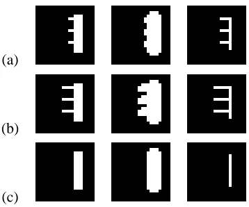
Building a real system that would track people over time, and creating a real world test and training sets are outside the scope of our current work. Instead we have simulated the situation using the rules stated below. We define six behavior models. Each behavior model has some freedom with respect to certain parameters. The first model, shown in Figure 1(a) is of straight trajectories. This model, as well as the other more complex ones, has the freedom to choose starting and ending points. The next two models, shown in Figures 1(b), 1(c), change their direction once or twice respectively. The exact location of the change can vary slightly as does the orientation of the new direction. The fourth model, shown in Figure 1(d), has a small arc. The starting point of the arc and its length can vary to some extent. The fifth model, shown in Figure 1(e), has a much wider arc, while the last model, shown in Figure 1(f), completes almost a full circle before continuing to its original direction. The exact parameters of the circular motion and its starting point can vary.

We used the Support Vector Machine (SVM) (Boser et al., 1992, Vapnik, 1998) algorithm for our classification engine. The SVM was given a training set of input matrices A1, ...,Al with la-bels y1, ...,yl where yi=±1, where the columns of a matrix Airepresent the trajectories of the i’th “instance” example. The input to the SVM algorithm is a “measurement” matrix M whose entries

Mi j=yiyjf(Ai,Aj) and the output is a set of “support vectors” which consist of the subset of in-stances which lie on the margin of the positive and negative examples. In our case, the support vectors are matrices. The classification of a new test example A is based on the evaluation of the function:

h(A) =sgn(

∑

where the sum is over the support matrices and µi are the corresponding Lagrange multipliers pro-vided by the algorithm. Note that it is crucial that our measure f() is a positive definite kernel because otherwise we could not have plugged it in the SVM.

(a) (b) (c)

(d) (e) (f)

Figure 1: Six models of trajectories. Each figure illustrates some of the variability within one spe-cific model. (a) straight line trajectories, (b) direction changes once along the trajectory, (c) direction changes twice, (d) trajectories with an arc, (e) trajectories with a wide arc, (f) trajectories which complete up to a full circle.

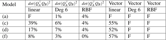
directions: left to right, right to left, top to bottom and bottom up. Each example contains seven trajectories. A homogeneous set is considered to be a set where all trajectories lie in one direction. An inhomogeneous set is considered to be a set where six trajectories lie in one direction and one trajectory lies in some other direction. We used 400 training examples and 100 test examples for each experiment. The results are shown in Table 1.

Model det(Q>AQB)2 det(Q>AQB)2 det(Q>AQB)2 Vector Vector Vector

linear Deg 6 RBF linear Deg 6 RBF

(a) F 1% 4% F F F

(c) 39% 6% 4% 55% F F

(d) 17% 7% 4% 52% F F

(f) 8% 3% 0% 57% F F

Table 1: Results of the first synthetic experiment. Table entries show the error rates for different experiments. The results are given for our proposed kernel for sets over a linear kernel, a polynomial kernel of degree 6, and for an RBF kernel and for the vector representation of the sets using the same kernels. Each row represents an experiment made using adifferent model of trajectories. “F” means that the SVM classifier failed to converge.

experiment made using a different model of trajectories. “F” means that the SVM classifier failed to converge. One can notice a striking difference between the set of vectors representation of the data compared to the 1-dimensional representation. With the set representation one can see a significant improvement when non-linear kernels are used (polynomial and RBF).

The second experiment was similar to the first one, but here we used the first three models together. In this experiment, a homogeneous set includes seven trajectories of the same randomly picked model of the three. All trajectories in a homogeneous set were oriented along the same direction. In an inhomogeneous set, on the other hand, there exists a single trajectory of a different model whose motion was oriented at a random direction which might or might not coincide with the direction of the other six trajectories (see Table 2, first row). We tried a “tougher” variation along the same experimental theme where all the trajectories (regular and irregular) extent from left to right (a single direction). As a result, the irregular trajectory is expressed only by the trajectory model and not by direction (see Table 2, second row).

Directions det(Q>_AQB)2 det(Q>AQB)2 det(Q>AQB)2 Vector Vector Vector

linear Deg 6 RBF linear Deg 6 RBF

4 26% 19% 7% 60% F F

1 F 40% 44% F F F

Table 2: Results for the second experiment, organized in a similar manner as in Table 1. In the first row the trajectories moved in one of four directions. The last row of results is for the case all trajectories were left to right.

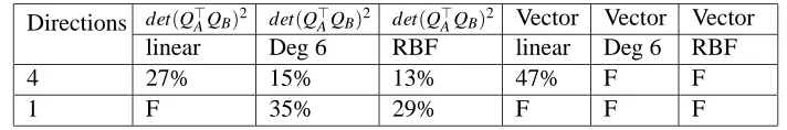
The third experiment was similar to the second one, only this time we used all six models as possible types of trajectories. Error rates are given in Table 3.

Directions det(Q>AQB)

2 _det(Q>

AQB)

2 _det(Q>

AQB)

2 _{Vector Vector Vector}

linear Deg 6 RBF linear Deg 6 RBF

4 27% 15% 13% 47% F F

1 F 35% 29% F F F

Table 3: Results for the third experiment, organized in a similar manner as in Table 2.

5.2 Face Recognition

In our second experimental example the goal was to recognize a face by matching video sequences. We ran a face tracker on 9 persons who were making head and facial movements in front of a camera. The result of the face tracker is an area of interest bounding the face which was scaled (up or down) to a fixed size of 35×47 per frame per person. The number of images per set varied from 30 to 200 frames per set. Since the tracker is not perfect (none of them are) especially against strong pose changes of the head, some of the elements of the set were not positioned properly on the face (Figure 2 second row).

Figure 2: Each pair of rows contains some of the extracted face images of the same person on different shots taken under different illumination. The sequences on the top two rows is a hard example that was not recognized by any method.

sets between the test set and the 9 training sets. The kernel principal angles was applied once on the original image space and once using a feature space representing the sixth order monomial expansion of the original input vectors. Since we are not constrained in this experiment to use a positive definite measure, we used the mean of the smallest 20 principal angles as the similarity measure between two video sequences (labeled as “meanθ” belowq). Note also that in this kind of experiment, the length of the video sequences can vary.

We compared our results to four other approaches for obtaining a similarity measure over sets. In the second approach (labeled “alt”), instead of computing the principal angles, we chose the angle between the closest vectors in the two sets. At first the two vectors (one from each set) which had the largest inner-product were picked. They were removed and we then picked the next pair and so on. This method is used as a “low cost substitute” for principal angles. The third method (labeled “NN”) measured the distance between every two sets as the distance in feature space between their closest elements. Recall that the distance in feature space between two vectors is:

d(φ(x),φ(x0))2=k(x,x) +k(x0,x0)−2k(x,x0).

The fourth method (labeled “20NN”) examined the 20 vectors in the union of the training sets which were closest to the vectors of the test set. The recognition process was based on a vote - the training set which contributed the most of these vectors was chosen. The last method we compared to was the method based on Kullback-Leibler divergence presented in Shakhnarovich et al. (2002).

One can see from Table 4 that our approach based on computing the principal angles in a feature space of sixth order monomials made only a single error out of 7 tests (the first two rows of Figure 2, where as all four other approaches performed poorly.

5.3 Kernel Jittering

Linear Deg 6

meanθ 2 1

Alt 4 4

NN 5 5

20NN 3 3

(Shakhnarovich et al., 2002)

4 NA

Table 4: Number of matching errors on face image sequences tested against various methods. The model dataset consisted of 9 image sequences representing 9 different people. The test set consisted of 7 new sequences (of the same people) and a match was conducted to find the closest training sequence. The first row shows the number of matching errors using Q−α

with a scoring function equal to the mean of the principal angles. When a sixth-degree polynomial kernel was used there was only one matching mistake (depicted in the first two rows of Figure 2). All other methods (see text) had a significantly higher number of matching errors.

section we compare the performance, on a toy problem, of such an approach to our positive definite kernel based on principal angles.

Consider the case of generating virtual examples in order to train the classifier to become invari-ant to line width (in the context of digit recognition). As an example, we are given three example vectors, each representing an image, and we generate two additional vectors per example by artifi-cially thinning and thickening the lines using morphological operators (see Figure 3). As a result we obtain three sets of vectors with three vectors each. A good matching-over-sets is one which will be invariant to line width. Note that unlike the case of invariance to translation, since these mor-phological operators are not symmetrical (information is lost) the matching has to be done between two sets rather than between a vector and a set. Finally note that the nearest neighbor approach is not positive definite (due to the asymmetry of the invariance relation).

We have computed a distance based on our positive definite kernel between every two sets based on underlying kernels of linear and polynomial types. We also computed the nearest neighbor dis-tance between the sets as the minimal disdis-tance between points in the sets using the same underlying kernels. The nearest-neighbor approach picked the pair “short comb” and “lines” as the most similar — regardless of the kernel being used (rows (a) and (c) in Figure 3). The kernel principal angles approach made the same judgment when using the original image space (consistent with the notion that the strength of the approach is based on the ability to work in feature space) but made the cor-rect judgment with the sixth degree monomial expansion kernel, i.e., determined that rows (a),(b) are the closest pair.

6. Summary

In this paper we have made three contributions:

(a)

(b)

(c)

Figure 3: Each row contains an image, the image after a morphological thick operator, and the image after a morphological thin operator. Nearest neighbor approach on this set yields that the set in the first row is closer to the set in the third row then to the set in the second row. Our positive definite kernel, which takes into account all the image space identified that the sets in the first and second row are more similar.

not exclusively so as we noted that “kernel jittering” is another case for similarity over sets of vectors.

• A kernel approach for the computation of principal angles in feature space. We noted that principal angles in the original input space is a fairly limited tool for comparing subspaces be-cause of the linearity assumption. However, the linearity assumption in the high-dimensional feature space allows for non-linearities in the input space thereby making the principal angles approach for matrix similarity a powerful tool for matching over sets.

• Introducing the function f(A,B)which forms a positive definite kernel. This result is impor-tant for making use of the similarity measure over matrices as a metric for optimal margin classifiers.

Acknowledgements

A preliminary version of this work has appeared as a conference paper (Wolf and Shashua, 2003). L. Wolf’s current address is at the Center of Biological and Computational Learning (CBCL), M.I.T., Cambridge, MA 02139. We would like to acknowledge support for this project from the Israeli Science Foundation (ISF grant 189/03). We would also like to thank Adi Shavit, Dana Segal and GenTech corporation for the use of their “head” detection and tracker software.

References

A.C. Aitken. Determinants and Matrices. nterscience Publishers Inc., 4 edition, 1946.

F.R. Bach and M.I. Jordan. Kernel independent component analysis. Journal of Machine Learning

Research, 3:1–48, 2002.

H. Baird. Document image defect models. In IAPR Workshop on Syntactic and Structural Pattern

Recognition, 1990.

Z. Biuk and S. Loncaric. Face recognition from multi-pose image sequence. In 2nd Int’l Symposium

on Image and Signal Processing and Analysis, 2001.

A. Bjork and G.H. Golub. Numerical methods for computing angles between linear subspaces.

Mathematics of Computation, 27(123):579–594, 1973.

B.E. Boser, I.M. Guyon, and V.N. Vapnik. A training algorithm for optimal margin classifier. In

Proc. 5th Workshop on Computational Learning Theory, pages 144–152, 1992.

R.A Brualdi, S. Friedland, and A. Pothen. The sparse basis problem and multilinear algebra. SIAM

Journal on Matrix Analysis and Applications, 16, 1995.

P.E. Caines. Linear Stochastic Systems. Wiley, NY, 1988.

D. DeCoste and B. Sch ¨olkopf. Training invariant support vector machines. Machine Learning, 46: 161–190, 2002.

G.J. Edwards, C.J. Taylor, and T.F. Cootes. Improving identification performance by integrating ev-idence from sequences. In Proceedings of the IEEE Conference on Computer Vision and Pattern

Recognition, 1999.

I.M. Gelfand and A.M. Yaglom. Calculation of the amount of information about a random function contained in another such function. Amer. Math. Soc. Translations, series 2, 12:199–246, 1959.

T.V. Gestel, J.A.K. Suykens, J. De Brabanter, B. De Moor, and J. Vandewalle. Kernel canonical correlation analysis and least squares support vector achines. In Int. Conf. on Artificial Neural

Networks, pages 384–389, Berlin, 2001.

R. Gittins. Cannonical analysis: A review with applications in ecology. Biomathematics, 12, 1985.

S. Gong, A. Psarrou, I. Katsoulis, and P. Palavouzis. Tracking and recognition of face sequences. In

H. Hotelling. Relations between two sets of variates. Biometrika, 28:321–372, 1936.

T. Kailath. A view of three decades of linear filtering theory. IEEE trans. on Information Theory, 20(2):146–181, 1974.

M. Kuss and T. Graepel. The geometry of kernel canonical correlation analysis. Technical Report 108, Max-Planck Institute for Biol. Cybernetics, May 2003.

C.S. MacInnes. The solution to a structured matrix approximation problem using grassman coordi-nates. SIAM Journal on Matrix Analysis and Applications, 21(2), 1999.

T. Melzer, M. Reiter, and H. Bischof. Nonlinear feature extraction using generalized canonical correlation analysis. In Int. Conf. on Artificial Neural Networks, pages 353–360, Berlin, 2001.

M.Turk and A.Pentland. Eigen faces for recognition. J. of Cognitive Neuroscience, 3(1), 1991.

T. Poggio and T. Vetter. Recognition and structure from one 2D model view: Observations on pro-totypes, object classes and symmetries. A.I. Memo No. 1347, Artificial Intelligence Laboratory, Massachusetts Institute of Technology, February 1992.

B. Sch¨olkopf and A.J. Smola. Learning with Kernels. MIT Press, Cambridge, MA, 2002.

G. Shakhnarovich, J.W. Fisher, and T. Darrell. Face recognition from long-term observations. In

Proceedings of the European Conference on Computer Vision, 2002.

P. Simard, B. Victorri, T. LeCun, and J. Denker. Tangent prop - a formalism for specifying selected invariances in an adaptive network. In Proceedings of the Conference on Neural Information

Processing Systems (NIPS), 1992.

V.N. Vapnik. The nature of statistical learning. Springer, 2nd edition, 1998.

L. Wolf and A. Shashua. Kernel principal angles for classification machines with applications to image sequence interpretation. In Proceedings of the IEEE Conference on Computer Vision and

Pattern Recognition, 2003.