A Kernel Two-Sample Test
Arthur Gretton∗ [email protected]
MPI for Intelligent Systems Spemannstrasse 38 72076 T¨ubingen, Germany
Karsten M. Borgwardt† [email protected] Machine Learning and Computational Biology Research Group
Max Planck Institutes T¨ubingen Spemannstrasse 38
72076 T¨ubingen, Germany
Malte J. Rasch‡ [email protected]
19 XinJieKouWai St.
State Key Laboratory of Cognitive Neuroscience and Learning, Beijing Normal University,
Beijing, 100875, P.R. China
Bernhard Sch¨olkopf [email protected] MPI for Intelligent Systems
Spemannstrasse 38 72076, T¨ubingen, Germany
Alexander Smola§ [email protected]
Yahoo! Research
2821 Mission College Blvd Santa Clara, CA 95054, USA
Editor: Nicolas Vayatis
Abstract
We propose a framework for analyzing and comparing distributions, which we use to construct sta-tistical tests to determine if two samples are drawn from different distributions. Our test statistic is the largest difference in expectations over functions in the unit ball of a reproducing kernel Hilbert space (RKHS), and is called the maximum mean discrepancy (MMD). We present two distribution-free tests based on large deviation bounds for the MMD, and a third test based on the asymptotic distribution of this statistic. The MMD can be computed in quadratic time, although efficient linear time approximations are available. Our statistic is an instance of an integral probability metric, and various classical metrics on distributions are obtained when alternative function classes are used in place of an RKHS. We apply our two-sample tests to a variety of problems, including attribute matching for databases using the Hungarian marriage method, where they perform strongly. Ex-cellent performance is also obtained when comparing distributions over graphs, for which these are the first such tests.
∗. Also at Gatsby Computational Neuroscience Unit, CSML, 17 Queen Square, London WC1N 3AR, UK. †. This work was carried out while K.M.B. was with the Ludwig-Maximilians-Universit¨at M¨unchen. ‡. This work was carried out while M.J.R. was with the Graz University of Technology.
Keywords: kernel methods, two-sample test, uniform convergence bounds, schema matching, integral probability metric, hypothesis testing
1. Introduction
We address the problem of comparing samples from two probability distributions, by proposing statistical tests of the null hypothesis that these distributions are equal against the alternative hy-pothesis that these distributions are different (this is called the two-sample problem). Such tests have application in a variety of areas. In bioinformatics, it is of interest to compare microarray data from identical tissue types as measured by different laboratories, to detect whether the data may be analysed jointly, or whether differences in experimental procedure have caused systematic differences in the data distributions. Equally of interest are comparisons between microarray data from different tissue types, either to determine whether two subtypes of cancer may be treated as statistically indistinguishable from a diagnosis perspective, or to detect differences in healthy and cancerous tissue. In database attribute matching, it is desirable to merge databases containing mul-tiple fields, where it is not known in advance which fields correspond: the fields are matched by maximising the similarity in the distributions of their entries.
We test whether distributions p and q are different on the basis of samples drawn from each of them, by finding a well behaved (e.g., smooth) function which is large on the points drawn from p, and small (as negative as possible) on the points from q. We use as our test statistic the difference between the mean function values on the two samples; when this is large, the samples are likely from different distributions. We call this test statistic the Maximum Mean Discrepancy (MMD).
Clearly the quality of the MMD as a statistic depends on the classFof smooth functions that define it. On one hand,Fmust be “rich enough” so that the population MMD vanishes if and only if p=q. On the other hand, for the test to be consistent in power,Fneeds to be “restrictive” enough for the empirical estimate of the MMD to converge quickly to its expectation as the sample size increases. We will use the unit balls in characteristic reproducing kernel Hilbert spaces (Fukumizu et al., 2008; Sriperumbudur et al., 2010b) as our function classes, since these will be shown to satisfy both of the foregoing properties. We also review classical metrics on distributions, namely the Kolmogorov-Smirnov and Earth-Mover’s distances, which are based on different function classes; collectively these are known as integral probability metrics (M¨uller, 1997). On a more practical note, the MMD has a reasonable computational cost, when compared with other two-sample tests: given m points sampled from p and n from q, the cost is O(m+n)2 time. We also propose a test statistic with a computational cost of O(m+n): the associated test can achieve a given Type II error at a lower overall computational cost than the quadratic-cost test, by looking at a larger volume of data.
We define three nonparametric statistical tests based on the MMD. The first two tests are distribution-free, meaning they make no assumptions regarding p and q, albeit at the expense of being conservative in detecting differences between the distributions. The third test is based on the asymptotic distribution of the MMD, and is in practice more sensitive to differences in distribution at small sample sizes. The present work synthesizes and expands on results of Gretton et al. (2007a,b) and Smola et al. (2007),1who in turn build on the earlier work of Borgwardt et al. (2006). Note that 1. In particular, most of the proofs here were not provided by Gretton et al. (2007a), but in an accompanying technical
the latter addresses only the third kind of test, and that the approach of Gretton et al. (2007a,b) is rigorous in its treatment of the asymptotic distribution of the test statistic under the null hypothesis. We begin our presentation in Section 2 with a formal definition of the MMD. We review the notion of a characteristic RKHS, and establish that whenFis a unit ball in a characteristic RKHS, then the population MMD is zero if and only if p=q. We further show that universal RKHSs in
the sense of Steinwart (2001) are characteristic. In Section 3, we give an overview of hypothesis testing as it applies to the two-sample problem, and review alternative test statistics, including the
L2 distance between kernel density estimates (Anderson et al., 1994), which is the prior approach closest to our work. We present our first two hypothesis tests in Section 4, based on two different bounds on the deviation between the population and empirical MMD. We take a different approach in Section 5, where we use the asymptotic distribution of the empirical MMD estimate as the basis for a third test. When large volumes of data are available, the cost of computing the MMD (quadratic in the sample size) may be excessive: we therefore propose in Section 6 a modified version of the MMD statistic that has a linear cost in the number of samples, and an associated asymptotic test. In Section 7, we provide an overview of methods related to the MMD in the statistics and machine learning literature. We also review alternative function classes for which the MMD defines a metric on probability distributions. Finally, in Section 8, we demonstrate the performance of MMD-based two-sample tests on problems from neuroscience, bioinformatics, and attribute matching using the Hungarian marriage method. Our approach performs well on high dimensional data with low sample size; in addition, we are able to successfully distinguish distributions on graph data, for which ours is the first proposed test.
A Matlab implementation of the tests is atwww.gatsby.ucl.ac.uk/∼gretton/mmd/mmd.htm.
2. The Maximum Mean Discrepancy
In this section, we present the maximum mean discrepancy (MMD), and describe conditions under which it is a metric on the space of probability distributions. The MMD is defined in terms of particular function spaces that witness the difference in distributions: we therefore begin in Section 2.1 by introducing the MMD for an arbitrary function space. In Section 2.2, we compute both the population MMD and two empirical estimates when the associated function space is a reproducing kernel Hilbert space, and in Section 2.3 we derive the RKHS function that witnesses the MMD for a given pair of distributions.
2.1 Definition of the Maximum Mean Discrepancy
Our goal is to formulate a statistical test that answers the following question:
Problem 1 Let x and y be random variables defined on a topological space X, with respective Borel probability measures p and q . Given observations X :={x1, . . . ,xm}and Y :={y1, . . . ,yn},
independently and identically distributed (i.i.d.) from p and q, respectively, can we decide whether p6=q?
Where there is no ambiguity, we use the shorthand notation Ex[f(x)]:=Ex∼p[f(x)]and Ey[f(y)]:=
Ey∼q[f(y)]to denote expectations with respect to p and q, respectively, where x∼p indicates x has
distribution p. To start with, we wish to determine a criterion that, in the population setting, takes on a unique and distinctive value only when p=q. It will be defined based on Lemma 9.3.2 of
Lemma 1 Let(X,d)be a metric space, and let p,q be two Borel probability measures defined on
X. Then p=q if and only if Ex(f(x)) =Ey(f(y))for all f ∈C(X), where C(X) is the space of
bounded continuous functions onX.
Although C(X)in principle allows us to identify p=q uniquely, it is not practical to work with such
a rich function class in the finite sample setting. We thus define a more general class of statistic, for as yet unspecified function classesF, to measure the disparity between p and q (Fortet and Mourier, 1953; M¨uller, 1997).
Definition 2 LetFbe a class of functions f :X→Rand let p,q,x,y,X,Y be defined as above. We define the maximum mean discrepancy (MMD) as
MMD[F,p,q]:=sup
f∈F
(Ex[f(x)]−Ey[f(y)]). (1)
In the statistics literature, this is known as an integral probability metric (M¨uller, 1997). A biased2 empirical estimate of the MMD is obtained by replacing the population expectations with empirical expectations computed on the samples X and Y ,
MMDb[F,X,Y]:=sup f∈F
1
m
m
∑
i=1 f(xi)−
1
n
n
∑
i=1 f(yi)
!
. (2)
We must therefore identify a function class that is rich enough to uniquely identify whether p=q,
yet restrictive enough to provide useful finite sample estimates (the latter property will be established in subsequent sections).
2.2 The MMD in Reproducing Kernel Hilbert Spaces
In the present section, we propose as our MMD function classFthe unit ball in a reproducing kernel Hilbert spaceH. We will provide finite sample estimates of this quantity (both biased and unbiased), and establish conditions under which the MMD can be used to distinguish between probability measures. Other possible function classesFare discussed in Sections 7.1 and 7.2.
We first review some properties ofH(Sch¨olkopf and Smola, 2002). SinceHis an RKHS, the operator of evaluationδxmapping f ∈Hto f(x)∈Ris continuous. Thus, by the Riesz
represen-tation theorem (Reed and Simon, 1980, Theorem II.4), there is a feature mappingφ(x) fromXto
Rsuch that f(x) =hf,φ(x)iH. This feature mapping takes the canonical formφ(x) =k(x,·)
(Stein-wart and Christmann, 2008, Lemma 4.19), where k(x1,x2) : X×X→Ris positive definite, and the notation k(x,·) indicates the kernel has one argument fixed at x, and the second free. Note in particular thathφ(x),φ(y)iH=k(x,y). We will generally use the more concise notationφ(x)for the
feature mapping, although in some cases it will be clearer to write k(x,·).
We next extend the notion of feature map to the embedding of a probability distribution: we will define an element µp ∈H such that Exf =hf,µpiH for all f ∈H, which we call the mean
embedding of p. Embeddings of probability measures into reproducing kernel Hilbert spaces are
well established in the statistics literature: see Berlinet and Thomas-Agnan (2004, Chapter 4) for further detail and references. We begin by establishing conditions under which the mean embedding
µpexists (Fukumizu et al., 2004, p. 93), (Sriperumbudur et al., 2010b, Theorem 1).
Lemma 3 If k(·,·)is measurable and Ex p
k(x,x)<∞then µp∈H.
Proof The linear operator Tpf :=Exf for all f ∈Fis bounded under the assumption, since
|Tpf|=|Exf| ≤Ex|f|=Ex|hf,φ(x)iH| ≤Ex p
k(x,x)kfkH
.
Hence by the Riesz representer theorem, there exists a µp∈Hsuch that Tpf=hf,µpiH. If we set
f =φ(t) =k(t,·), we obtain µp(t) =hµp,k(t,·)iH=Exk(t,x): in other words, the mean embedding
of the distribution p is the expectation under p of the canonical feature map.
We next show that the MMD may be expressed as the distance in H between mean embeddings (Borgwardt et al., 2006).
Lemma 4 Assume the condition in Lemma 3 for the existence of the mean embeddings µp, µq is
satisfied. Then
MMD2[F,p,q] =µp−µq 2H.
Proof
MMD2[F,p,q] =
"
sup
kfkH≤1
(Ex[f(x)]−Ey[f(y)]) #2
=
"
sup
kfkH≤1
µp−µq,f
H #2
= µp−µq 2
H.
We now establish a condition on the RKHSH under which the mean embedding µp is injective,
which indicates that MMD[F,p,q] =0 is a metric3 on the Borel probability measures onX. Evi-dently, this property will not hold for allH: for instance, a polynomial RKHS of degree two cannot distinguish between distributions with the same mean and variance, but different kurtosis (Sriperum-budur et al., 2010b, Example 3). The MMD is a metric, however, whenHis a universal RKHSs, defined on a compact metric space X. Universality requires that k(·,·) be continuous, andH be dense in C(X)with respect to the L∞norm. Steinwart (2001) proves that the Gaussian and Laplace RKHSs are universal.
Theorem 5 LetFbe a unit ball in a universal RKHSH, defined on the compact metric spaceX, with associated continuous kernel k(·,·). Then MMD[F,p,q] =0 if and only if p=q.
Proof The proof follows Cortes et al. (2008, Supplementary Appendix), whose approach is clearer than the original proof of Gretton et al. (2008a, p. 4).4 First, it is clear that p= q implies 3. According to Dudley (2002, p. 26) a metric d(x,y)satisfies the following four properties: symmetry, triangle
in-equality, d(x,x) =0, and d(x,y) =0 =⇒ x=y. A pseudo-metric only satisfies the first three properties.
4. Note that the proof of Cortes et al. (2008) requires an application the of dominated convergence theorem, rather than using the Riesz representation theorem to show the existence of the mean embeddings µpand µqas we did in Lemma
MMD{F,p,q}is zero. We now prove the converse. By the universality ofH, for any givenε>0 and f ∈C(X)there exists a g∈Hsuch that
kf−gk∞≤ε.
We next make the expansion
|Exf(x)−Ey(f(y))| ≤ |Exf(x)−Exg(x)|+|Exg(x)−Eyg(y)|+|Eyg(y)−Eyf(y)|.
The first and third terms satisfy
|Exf(x)−Exg(x)| ≤Ex|f(x)−g(x)| ≤ε.
Next, write
Exg(x)−Eyg(y) =
g,µp−µq
H=0,
since MMD{F,p,q}=0 implies µp=µq. Hence
|Exf(x)−Ey(f(y))| ≤2ε
for all f ∈C(X)andε>0, which implies p=q by Lemma 1.
While our result establishes the mapping µpis injective for universal kernels on compact domains,
this result can also be shown in more general cases. Fukumizu et al. (2008) introduces the notion of characteristic kernels, these being kernels for which the mean map is injective. Fukumizu et al. establish that Gaussian and Laplace kernels are characteristic onRd, and thus that the associated MMD is a metric on distributions for this domain. Sriperumbudur et al. (2008, 2010b) and Sripe-rumbudur et al. (2011a) further explore the properties of characteristic kernels, providing a simple condition to determine whether translation invariant kernels are characteristic, and investigating the relation between universal and characteristic kernels on non-compact domains.
Given we are in an RKHS, we may easily obtain of the squared MMD,µp−µq
2H, in terms of kernel functions, and a corresponding unbiased finite sample estimate.
Lemma 6 Given x and x′independent random variables with distribution p, and y and y′ indepen-dent random variables with distribution q, the squared population MMD is
MMD2[F,p,q] =Ex,x′
k(x,x′)−2Ex,y[k(x,y)] +Ey,y′
k(y,y′),
where x′is an independent copy of x with the same distribution, and y′is an independent copy of y. An unbiased empirical estimate is a sum of two U-statistics and a sample average,
MMD2u[F,X,Y] = 1 m(m−1)
m
∑
i=1
m
∑
j6=i
k(xi,xj) +
1
n(n−1)
n
∑
i=1
n
∑
j6=i
k(yi,yj)
−mn2
m
∑
i=1
n
∑
j=1
k(xi,yj). (3)
When m=n, a slightly simpler empirical estimate may be used. Let Z := (z1, . . . ,zm)be m i.i.d.
random variables, where z := (x,y)∼p×q (i.e., x and y are independent). An unbiased estimate of
MMD2is
MMD2u[F,X,Y] = 1 (m)(m−1)
m
∑
i6=j
which is a one-sample U-statistic with
h(zi,zj):=k(xi,xj) +k(yi,yj)−k(xi,yj)−k(xj,yi).
Proof Starting from the expression for MMD2[F,p,q]in Lemma 4, MMD2[F,p,q] = µp−µq
2
H
= hµp,µpiH+
µq,µq
H−2
µp,µq
H
= Ex,x′φ(x),φ(x′)H+Ey,y′φ(y),φ(y′)H−2Ex,yhφ(x),φ(y)iH,
The proof is completed by applyinghφ(x),φ(x′)iH=k(x,x′); the empirical estimates follow straight-forwardly, by replacing the population expectations with their corresponding U-statistics and sample averages. This statistic is unbiased following Serfling (1980, Chapter 5).
Note that MMD2u may be negative, since it is an unbiased estimator of(MMD[F,p,q])2. The only terms missing to ensure nonnegativity, however, are h(zi,zi), which were removed to remove
spuri-ous correlations between observations. Consequently we have the bound
MMD2u+ 1 m(m−1)
m
∑
i=1
k(xi,xi) +k(yi,yi)−2k(xi,yi)≥0.
Moreover, while the empirical statistic for m=n is an unbiased estimate of MMD2, it does not have minimum variance, since we ignore the cross-terms k(xi,yi), of which there are O(n). From (3),
however, we see the minimum variance estimate is almost identical (Serfling, 1980, Section 5.1.4). The biased statistic in (2) may also be easily computed following the above reasoning. Substi-tuting the empirical estimates µX :=m1∑mi=1φ(xi)and µY := 1n∑ni=1φ(yi)of the feature space means
based on respective samples X and Y , we obtain
MMDb[F,X,Y] = "
1
m2
m
∑
i,j=1
k(xi,xj)−
2
mn
m,n
∑
i,j=1
k(xi,yj) +
1
n2
n
∑
i,j=1
k(yi,yj) #1
2
. (5)
Note that the U-statistics of (3) have been replaced by V-statistics. Intuitively we expect the empir-ical test statistic MMD[F,X,Y], whether biased or unbiased, to be small if p=q, and large if the
distributions are far apart. It costs O((m+n)2)time to compute both statistics. 2.3 Witness Function of the MMD for RKHSs
We define the witness function f∗ to be the RKHS function attaining the supremum in (1), and its empirical estimate ˆf∗ to be the function attaining the supremum in (2). From the reasoning in Lemma 4, it is clear that
f∗(t) ∝ φ(t),µp−µq
H = Ex[k(x,t)]−Ey[k(y,t)],
ˆ
f∗(t) ∝ hφ(t),µX−µYiH = m1∑mi=1k(xi,t)−1n∑ni=1k(yi,t).
where we have defined µX =m−1∑mi=1φ(xi), and µY by analogy. The result follows since the unit
vector v maximizinghv,xiHin a Hilbert space is v=x/kxkH.
−6 −4 −2 0 2 4 6 −0.6
−0.4 −0.2 0 0.2 0.4 0.6 0.8
t
P
ro
b
.
d
en
si
ti
es
a
n
d
ˆf
∗(
t
)
ˆ f∗ p(Gau ss) q(L ap l ace)
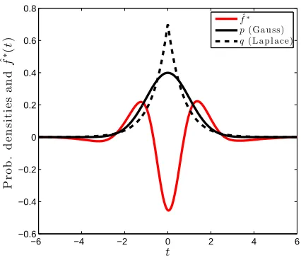
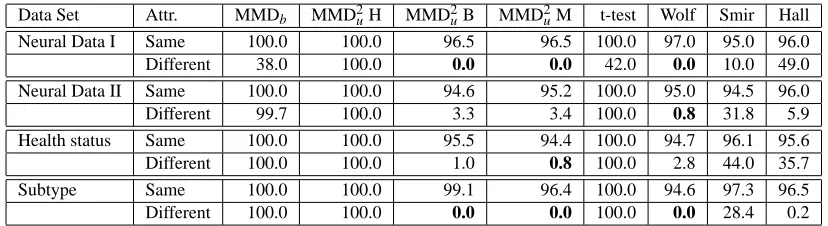
Figure 1: Illustration of the function maximizing the mean discrepancy in the case where a Gaussian is being compared with a Laplace distribution. Both distributions have zero mean and unit variance. The function ˆf∗that witnesses the MMD has been scaled for plotting purposes, and was computed empirically on the basis of 2×10⁴samples, using a Gaussian kernel withσ=0.5.
and q Laplacian. We choseFto be the unit ball in a Gaussian RKHS. The empirical estimate ˆf∗
of the function f∗ that witnesses the MMD—in other words, the function maximizing the mean discrepancy in (1)—is smooth, negative where the Laplace density exceeds the Gaussian density (at the center and tails), and positive where the Gaussian density is larger. The magnitude of ˆf∗ is a direct reflection of the amount by which one density exceeds the other, insofar as the smoothness constraint permits it.
3. Background Material
We now present three background results. First, we introduce the terminology used in statistical hypothesis testing. Second, we demonstrate via an example that even for tests which have asymp-totically no error, we cannot guarantee performance at any fixed sample size without making as-sumptions about the distributions. Third, we review some alternative statistics used in comparing distributions, and the associated two-sample tests (see also Section 7 for an overview of additional integral probability metrics).
3.1 Statistical Hypothesis Testing
samples X∼p of size m and Y∼q of size n, the statistical test,T(X,Y):Xm×Xn7→ {0,1}is used
to distinguish between the null hypothesisH0 : p=q and the alternative hypothesisHA : p6=q.
This is achieved by comparing the test statistic5 MMD[F,X,Y]with a particular threshold: if the threshold is exceeded, then the test rejects the null hypothesis (bearing in mind that a zero population MMD indicates p=q). The acceptance region of the test is thus defined as the set of real numbers
below the threshold. Since the test is based on finite samples, it is possible that an incorrect answer will be returned. A Type I error is made when p=q is rejected based on the observed samples,
despite the null hypothesis having generated the data. Conversely, a Type II error occurs when
p=q is accepted despite the underlying distributions being different. The levelα of a test is an upper bound on the probability of a Type I error: this is a design parameter of the test which must be set in advance, and is used to determine the threshold to which we compare the test statistic (finding the test threshold for a given α is the topic of Sections 4 and 5). The power of a test against a particular member of the alternative classHA(i.e., a specific(p,q)such that p6=q) is the
probability of wrongly accepting p=q in this instance. A consistent test achieves a levelα, and a Type II error of zero, in the large sample limit. We will see that the tests proposed in this paper are consistent.
3.2 A Negative Result
Even if a test is consistent, it is not possible to distinguish distributions with high probability at a given, fixed sample size (i.e., to provide guarantees on the Type II error), without prior assumptions as to the nature of the difference between p and q. This is true regardless of the two-sample test used. There are several ways to illustrate this, which each give insight into the kinds of differences that might be undetectable for a given number of samples. The following example6 is one such illustration.
Example 1 Assume we have a distribution p from which we have drawn m i.i.d. observations. We construct a distribution q by drawing m2 i.i.d. observations from p, and defining a discrete distribution over these m2 instances with probability m−2 each. It is easy to check that if we now draw m observations from q, there is at least a mm2mm!2m>1−e−1>0.63 probability that we thereby
obtain an m sample from p. Hence no test will be able to distinguish samples from p and q in this case. We could make the probability of detection arbitrarily small by increasing the size of the sample from which we construct q.
3.3 Previous Work
We next give a brief overview of some earlier approaches to the two sample problem for multivariate data. Since our later experimental comparison is with respect to certain of these methods, we give abbreviated algorithm names in italics where appropriate: these should be used as a key to the tables in Section 8.
5. This may be biased or unbiased.
3.3.1 L2DISTANCE BETWEENPARZENWINDOWESTIMATES
The prior work closest to the current approach is the Parzen window-based statistic of Anderson et al. (1994). We begin with a short overview of the Parzen window estimate and its properties (Silverman, 1986), before proceeding to a comparison with the RKHS approach. We assume a distribution p onRd, which has an associated density function f
p. The Parzen window estimate of
this density from an i.i.d. sample X of size m is
ˆ
fp(x) =
1
m
m
∑
i=1
κ(xi−x), whereκsatisfies Z
Xκ(x)dx=1 andκ(x)≥0.
We may rescaleκaccording toh1d mκ
x hm
for a bandwidth parameter hm. To simplify the discussion,
we use a single bandwidth hm+nfor both ˆfpand ˆfq. Assuming m/n is bounded away from zero and
infinity, consistency of the Parzen window estimates for fpand fqrequires
lim
m,n→∞h d
m+n=0 and mlim,n
→∞(m+n)h d
m+n=∞. (6)
We now show the L2distance between Parzen windows density estimates is a special case of the bi-ased MMD in Equation (5). Denote by Dr(p,q):=
fp−fq
rthe Lrdistance between the densities
fpand fqcorresponding to the distributions p and q, respectively. For r=1 the distance Dr(p,q)is
known as the L´evy distance (Feller, 1971), and for r=2 we encounter a distance measure derived from the Renyi entropy (Gokcay and Principe, 2002). Assume that ˆfp and ˆfq are given as kernel
density estimates with kernelκ(x−x′), that is, ˆfp(x) =m−1∑mi=1κ(xi−x)and ˆfq(y)is defined by
analogy. In this case
D2(fˆp,fˆq)2= Z "
1
m
m
∑
i=1
κ(xi−z)−
1
n
n
∑
i=1
κ(yi−z) #2
dz
= 1 m2
m
∑
i,j=1
k(xi−xj) +
1
n2
n
∑
i,j=1
k(yi−yj)−
2
mn
m,n
∑
i,j=1
k(xi−yj),
where k(x−y) =Rκ(x−z)κ(y−z)dz. By its definition k(x−y)is an RKHS kernel, as it is an inner product betweenκ(x−z)andκ(y−z)on the domainX.
We now describe the asymptotic performance of a two-sample test using the statistic D2(fˆp,fˆq)2.
We consider the power of the test under local departures from the null hypothesis. Anderson et al. (1994) define these to take the form
fq= fp+δg, (7)
whereδ∈R, and g is a fixed, bounded, integrable function chosen to ensure that fqis a valid density
for sufficiently small|δ|. Anderson et al. consider two cases: the kernel bandwidth converging to zero with increasing sample size, ensuring consistency of the Parzen window estimates of fpand
fq; and the case of a fixed bandwidth. In the former case, the minimum distance with which the test
can discriminate fpfrom fq is7δ= (m+n)−1/2h−md+/n2. In the latter case, this minimum distance is
δ= (m+n)−1/2, under the assumption that the Fourier transform of the kernelκdoes not vanish 7. Formally, define sαas a threshold for the statistic D2 fˆp,fˆq
2
, chosen to ensure the test has levelα, and letδ= (m+n)−1/2h−d/2
on an interval (Anderson et al., 1994, Section 2.4), which implies the kernel k is characteristic (Sriperumbudur et al., 2010b). The power of the L2test against local alternatives is greater when the kernel is held fixed, since for any rate of decrease of hm+n with increasing sample size,δwill
decrease more slowly than for a fixed kernel.
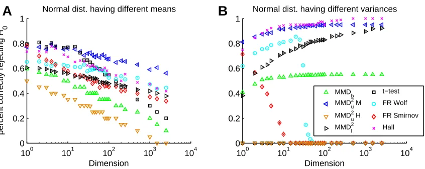
An RKHS-based approach generalizes the L2statistic in a number of important respects. First, we may employ a much larger class of characteristic kernels that cannot be written as inner products between Parzen windows: several examples are given by Steinwart (2001, Section 3) and Micchelli et al. (2006, Section 3) (these kernels are universal, hence characteristic). We may further generalize to kernels on structured objects such as strings and graphs (Sch¨olkopf et al., 2004), as done in our experiments (Section 8). Second, even when the kernel may be written as an inner product of Parzen windows onRd, the D22statistic with fixed bandwidth no longer converges to an L2distance between probability density functions, hence it is more natural to define the statistic as an integral probability metric for a particular RKHS, as in Definition 2. Indeed, in our experiments, we obtain good performance in experimental settings where the dimensionality greatly exceeds the sample size, and density estimates would perform very poorly8 (for instance the Gaussian toy example in Figure 5B, for which performance actually improves when the dimensionality increases; and the microarray data sets in Table 1). This suggests it is not necessary to solve the more difficult problem of density estimation in high dimensions to do two-sample testing.
Finally, the kernel approach leads us to establish consistency against a larger class of local alternatives to the null hypothesis than that considered by Anderson et al. In Theorem 13, we prove consistency against a class of alternatives encoded in terms of the mean embeddings of p and q, which applies to any domain on which RKHS kernels may be defined, and not only densities onRd. This more general approach also has interesting consequences for distributions onRd: for instance, a local departure fromH0 occurs when p and q differ at increasing frequencies in their respective characteristic functions. This class of local alternatives cannot be expressed in the formδg for fixed g, as in (7). We discuss this issue further in Section 5.
3.3.2 MMDFORMULTINOMIALS
Assume a finite domainX:={1, . . . ,d}, and define the random variables x and y onXsuch that
pi:=P(x=i)and qj:=P(y=j). We embed x into an RKHSHvia the feature mappingφ(x):=ex,
where esis the unit vector inRd taking value 1 in dimension s, and zero in the remaining entries.
The kernel is the usual inner product onRd. In this case,
MMD2[F,p,q] =kp−qk2Rd = d
∑
i=1
(pi−qi)2. (8)
Harchaoui et al. (2008, Section 1, long version) note that this L2statistic may not be the best choice for finite domains, citing a result of Lehmann and Romano (2005, Theorem 14.3.2) that Pearson’s
assuming conditions (6), the limit
π(c):= lim (m+n)→∞PrHA
D2 fˆp,fˆq 2
>sα
is well-defined, and satisfiesα<π(c)<1 for 0<|c|<∞, andπ(c)→1 as c→∞.
8. The L2error of a kernel density estimate converges as O(n−4/(4+d))when the optimal bandwidth is used (Wasserman,
Chi-squared statistic is optimal for the problem of goodness of fit testing for multinomials.9 It would be of interest to establish whether an analogous result holds for two-sample testing in a wider class of RKHS feature spaces.
3.3.3 FURTHERMULTIVARIATETWO-SAMPLETESTS
Biau and Gyorfi (2005) (Biau) use as their test statistic the L1 distance between discretized esti-mates of the probabilities, where the partitioning is refined as the sample size increases. This space partitioning approach becomes difficult or impossible for high dimensional problems, since there are too few points per bin. For this reason, we use this test only for low-dimensional problems in our experiments.
A generalisation of the Wald-Wolfowitz runs test to the multivariate domain was proposed and analysed by Friedman and Rafsky (1979) and Henze and Penrose (1999) (FR Wolf), and involves counting the number of edges in the minimum spanning tree over the aggregated data that connect points in X to points in Y . The resulting test relies on the asymptotic normality of the test statistic, and is not distribution-free under the null hypothesis for finite samples (the test threshold depends on p, as with our asymptotic test in Section 5; by contrast, our tests in Section 4 are distribution-free). The computational cost of this method using Kruskal’s algorithm is O((m+n)2log(m+n)), although more modern methods improve on the log(m+n) term: see Chazelle (2000) for details. Friedman and Rafsky (1979) claim that calculating the matrix of distances, which costs O((m+n)2), dominates their computing time; we return to this point in our experiments (Section 8). Two possible generalisations of the Kolmogorov-Smirnov test to the multivariate case were studied by Bickel (1969) and Friedman and Rafsky (1979). The approach of Friedman and Rafsky (FR Smirnov) in this case again requires a minimal spanning tree, and has a similar cost to their multivariate runs test.
A more recent multivariate test was introduced by Rosenbaum (2005). This entails computing the minimum distance non-bipartite matching over the aggregate data, and using the number of pairs containing a sample from both X and Y as a test statistic. The resulting statistic is distribution-free under the null hypothesis at finite sample sizes, in which respect it is superior to the Friedman-Rafsky test; on the other hand, it costs O((m+n)3) to compute. Another distribution-free test (Hall) was proposed by Hall and Tajvidi (2002): for each point from p, it requires computing the
closest points in the aggregated data, and counting how many of these are from q (the procedure is repeated for each point from q with respect to points from p). As we shall see in our experimental comparisons, the test statistic is costly to compute; Hall and Tajvidi consider only tens of points in their experiments.
4. Tests Based on Uniform Convergence Bounds
In this section, we introduce two tests for the two-sample problem that have exact performance guarantees at finite sample sizes, based on uniform convergence bounds. The first, in Section 4.1, uses the McDiarmid (1989) bound on the biased MMD statistic, and the second, in Section 4.2, uses a Hoeffding (1963) bound for the unbiased statistic.
4.1 Bound on the Biased Statistic and Test
We establish two properties of the MMD, from which we derive a hypothesis test. First, we show that regardless of whether or not p=q, the empirical MMD converges in probability at rate O((m+ n)−12)to its population value. This shows the consistency of statistical tests based on the MMD.
Second, we give probabilistic bounds for large deviations of the empirical MMD in the case p=q.
These bounds lead directly to a threshold for our first hypothesis test. We begin by establishing the convergence of MMDb[F,X,Y]to MMD[F,p,q]. The following theorem is proved in A.2.
Theorem 7 Let p,q,X,Y be defined as in Problem 1, and assume 0≤k(x,y)≤K. Then
PrX,Y n
|MMDb[F,X,Y]−MMD[F,p,q]|>2
(K/m)12+ (K/n) 1 2
+εo≤2 exp2K−(εm2mn+n),
where PrX,Y denotes the probability over the m-sample X and n-sample Y .
Our next goal is to refine this result in a way that allows us to define a test threshold under the null hypothesis p=q. Under this circumstance, the constants in the exponent are slightly improved. The
following theorem is proved in Appendix A.3.
Theorem 8 Under the conditions of Theorem 7 where additionally p=q and m=n,
MMDb[F,X,Y]≤m− 1 2
q
2Ex,x′[k(x,x)−k(x,x′)]
| {z }
B1(F,p)
+ε≤(2K/m)1/2
| {z }
B2(F,p)
+ε,
both with probability at least 1−exp
−ε4K2m
.
In this theorem, we illustrate two possible bounds B1(F,p)and B2(F,p)on the bias in the empirical estimate (5). The first inequality is interesting inasmuch as it provides a link between the bias bound
B1(F,p)and kernel size (for instance, if we were to use a Gaussian kernel with largeσ, then k(x,x) and k(x,x′)would likely be close, and the bias small). In the context of testing, however, we would need to provide an additional bound to show convergence of an empirical estimate of B1(F,p)to its population equivalent. Thus, in the following test for p=q based on Theorem 8, we use B2(F,p) to bound the bias.10
Corollary 9 A hypothesis test of levelαfor the null hypothesis p=q, that is, for MMD[F,p,q] =0,
has the acceptance region MMDb[F,X,Y]< p
2K/m
1+p2 logα−1.
We emphasize that this test is distribution-free: the test threshold does not depend on the particular distribution that generated the sample. Theorem 7 guarantees the consistency of the test against fixed alternatives, and that the Type II error probability decreases to zero at rate O m−1/2, assuming m= n. To put this convergence rate in perspective, consider a test of whether two normal distributions
have equal means, given they have unknown but equal variance (Casella and Berger, 2002, Exercise 8.41). In this case, the test statistic has a Student-t distribution with n+m−2 degrees of freedom, and its Type II error probability converges at the same rate as our test.
It is worth noting that bounds may be obtained for the deviation between population mean embeddings µp and the empirical embeddings µX in a completely analogous fashion. The proof
requires symmetrization by means of a ghost sample, that is, a second set of observations drawn from the same distribution. While not the focus of the present paper, such bounds can be used to perform inference based on moment matching (Altun and Smola, 2006; Dud´ık and Schapire, 2006; Dud´ık et al., 2004).
4.2 Bound on the Unbiased Statistic and Test
The previous bounds are of interest since the proof strategy can be used for general function classes with well behaved Rademacher averages (see Sriperumbudur et al., 2010a). WhenFis the unit ball in an RKHS, however, we may very easily define a test via a convergence bound on the unbiased statistic MMD2uin Lemma 4. We base our test on the following theorem, which is a straightforward application of the large deviation bound on U-statistics of Hoeffding (1963, p. 25).
Theorem 10 Assume 0≤k(xi,xj)≤K, from which it follows−2K≤h(zi,zj)≤2K. Then
PrX,Y
MMD2u(F,X,Y)−MMD2(F,p,q)>t ≤exp
−t2m2 8K2
where m2:=⌊m/2⌋(the same bound applies for deviations of−t and below). A consistent statistical test for p=q using MMD2uis then obtained.
Corollary 11 A hypothesis test of levelαfor the null hypothesis p=q has the acceptance region
MMD2u<(4K/√m)plog(α−1).
This test is distribution-free. We now compare the thresholds of the above test with that in Corollary 9. We note first that the threshold for the biased statistic applies to an estimate of MMD, whereas that for the unbiased statistic is for an estimate of MMD2. Squaring the former threshold to make the two quantities comparable, the squared threshold in Corollary 9 decreases as m−1, whereas the threshold in Corollary 11 decreases as m−1/2. Thus for sufficiently large11m, the McDiarmid-based
threshold will be lower (and the associated test statistic is in any case biased upwards), and its Type II error will be better for a given Type I bound. This is confirmed in our Section 8 experiments. Note, however, that the rate of convergence of the squared, biased MMD estimate to its population value remains at 1/√m (bearing in mind we take the square of a biased estimate, where the bias
term decays as 1/√m).
Finally, we note that the bounds we obtained in this section and the last are rather conservative for a number of reasons: first, they do not take the actual distributions into account. In fact, they are finite sample size, distribution-free bounds that hold even in the worst case scenario. The bounds could be tightened using localization, moments of the distribution, etc.: see, for example, Bousquet et al. (2005) and de la Pe˜na and Gin´e (1999). Any such improvements could be plugged straight into Theorem 19. Second, in computing bounds rather than trying to characterize the distribution of MMD(F,X,Y)explicitly, we force our test to be conservative by design. In the following we aim for an exact characterization of the asymptotic distribution of MMD(F,X,Y)instead of a bound. While this will not satisfy the uniform convergence requirements, it leads to superior tests in practice.
5. Test Based on the Asymptotic Distribution of the Unbiased Statistic
We propose a third test, which is based on the asymptotic distribution of the unbiased estimate of MMD2in Lemma 6. This test uses the asymptotic distribution of MMD2uunderH0, which follows from results of Anderson et al. (1994, Appendix) and Serfling (1980, Section 5.5.2): see Appendix B.1 for the proof.
Theorem 12 Let ˜k(xi,xj)be the kernel between feature space mappings from which the mean
em-bedding of p has been subtracted,
˜k(xi,xj) := φ(
xi)−µp,φ(xj)−µp
H
= k(xi,xj)−Exk(xi,x)−Exk(x,xj) +Ex,x′k(x,x′), (9)
where x′is an independent copy of x drawn from p. Assume ˜k∈L2(X×X,p×p)(i.e., the centred kernel is square integrable, which is true for all p when the kernel is bounded), and that for t= m+n, limm,n→∞m/t→ρxand limm,n→∞n/t→ρy:= (1−ρx)for fixed 0<ρx<1. Then underH0, MMD2uconverges in distribution according to
tMMD2u[F,X,Y]→
D ∞
∑
l=1 λl
h
(ρ−1/2
x al−ρ−y1/2bl)2−(ρxρy)−1 i
, (10)
where al ∼N(0,1)and bl∼N(0,1)are infinite sequences of independent Gaussian random
vari-ables, and theλi are eigenvalues of Z
X˜k
(x,x′)ψi(x)d p(x) =λiψi(x′).
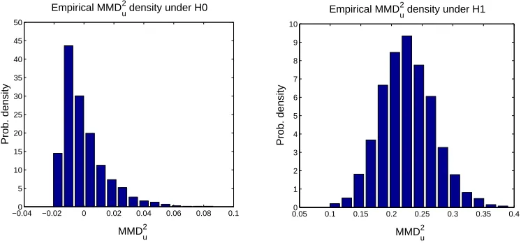
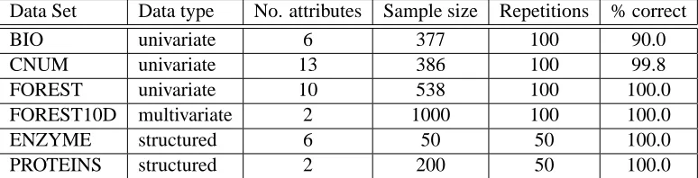
We illustrate the MMD density under both the null and alternative hypotheses by approximating it empirically for p=q and p6=q. Results are plotted in Figure 2.
Our goal is to determine whether the empirical test statistic MMD2uis so large as to be outside the 1−αquantile of the null distribution in (10), which gives a levelαtest. Consistency of this test against local departures from the null hypothesis is provided by the following theorem, proved in Appendix B.2.
Theorem 13 Defineρx,ρy, and t as in Theorem 12, and write µq=µp+gt, where gt∈His chosen
such that µp+gtremains a valid mean embedding, andkgtkHis made to approach zero as t→∞to
describe local departures from the null hypothesis. ThenkgtkH=ct−1/2is the minimum distance
between µpand µqdistinguishable by the test.
An example of a local departure from the null hypothesis is described earlier in the discussion of the L2 distance between Parzen window estimates (Section 3.3.1). The class of local alternatives considered in Theorem 13 is more general, however: for instance, Sriperumbudur et al. (2010b, Section 4) and Harchaoui et al. (2008, Section 5, long version) give examples of classes of pertur-bations gt with decreasing RKHS norm. These perturbations have the property that p differs from q
at increasing frequencies, rather than simply with decreasing amplitude.
−0.040 −0.02 0 0.02 0.04 0.06 0.08 0.1 5
10 15 20 25 30 35 40 45 50
Empirical MMD2
u density under H0
MMD2 u
Prob. density
0.050 0.1 0.15 0.2 0.25 0.3 0.35 0.4 1
2 3 4 5 6 7 8 9 10
Empirical MMD2
u density under H1
MMD2 u
Prob. density
Figure 2: Left: Empirical distribution of the MMD underH0, with p and q both Gaussians with unit standard deviation, using 50 samples from each. Right: Empirical distribution of the MMD underHA, with p a Laplace distribution with unit standard deviation, and q
a Laplace distribution with standard deviation 3√2, using 100 samples from each. In both cases, the histograms were obtained by computing 2000 independent instances of the MMD.
distribution by fitting Pearson curves to its first four moments (Johnson et al., 1994, Section 18.8). Taking advantage of the degeneracy of the U-statistic, we obtain for m=n
EMMD2u2
= 2
m(m−1)Ez,z′
h2(z,z′) and EMMD2u3= 8(m−2)
m2(m−1)2Ez,z′
h(z,z′)Ez′′ h(z,z′′)h(z′,z′′)+O(m−4) (11)
(see Appendix B.3), where h(z,z′)is defined in Lemma 6, z= (x,y)∼p×q where x and y are
inde-pendent, and z′,z′′are independent copies of z. The fourth moment EMMD2u4
is not computed,
since it is both very small, O(m−4), and expensive to calculate, O(m4). Instead, we replace the kur-tosis12with a lower bound due to Wilkins (1944), kurt MMD2u≥ skew MMD2u2+1. In Figure 3, we illustrate the Pearson curve fit to the null distribution: the fit is good in the upper quantiles of the distribution, where the test threshold is computed. Finally, we note that two alternative empiri-cal estimates of the null distribution have more recently been proposed by Gretton et al. (2009): a consistent estimate, based on an empirical computation of the eigenvaluesλl in (10); and an
alter-native Gamma approximation to the null distribution, which has a smaller computational cost but is generally less accurate. Further detail and experimental comparisons are given by Gretton et al.
12. The kurtosis is defined in terms of the fourth and second moments as kurt MMD2u
= E
[MMD2
u] 4
h
E[MMD2 u]
−0.020 0 0.02 0.04 0.06 0.08 0.1 0.12 0.2
0.4 0.6 0.8 1
CDF of the MMD and Pearson fit
t
P(MMD
2 < t) u
Emp. CDF Pearson
Figure 3: Illustration of the empirical CDF of the MMD and a Pearson curve fit. Both p and q were Gaussian with zero mean and unit variance, and 50 samples were drawn from each. The empirical CDF was computed on the basis of 1000 randomly generated MMD values. To ensure the quality of fit was determined only by the accuracy of the Pearson approxima-tion, the moments used for the Pearson curves were also computed on the basis of these 1000 samples. The MMD used a Gaussian kernel withσ=0.5.
6. A Linear Time Statistic and Test
The MMD-based tests are already more efficient than the O(m2log m)and O(m3)tests described in Section 3.3.3 (assuming m=n for conciseness). It is still desirable, however, to obtain O(m)tests which do not sacrifice too much statistical power. Moreover, we would like to obtain tests which have O(1) storage requirements for computing the test statistic, in order to apply the test to data streams. We now describe how to achieve this by computing the test statistic using a subsampling of the terms in the sum. The empirical estimate in this case is obtained by drawing pairs from X and
Y respectively without replacement.
Lemma 14 Define m2:=⌊m/2⌋, assume m=n, and define h(z1,z2)as in Lemma 6. The estimator
MMD2l[F,X,Y]:= 1 m2
m2
∑
i=1
h((x2i−1,y2i−1),(x2i,y2i))
can be computed in linear time, and is an unbiased estimate of MMD2[F,p,q].
While it is expected that MMD2l has higher variance than MMD2u(as we will see explicitly later), it is computationally much more appealing. In particular, the statistic can be used in stream computa-tions with need for only O(1)memory, whereas MMD2u requires O(m)storage and O(m2)time to compute the kernel h on all interacting pairs.
Theorem 15 Assume 0≤k(xi,xj)≤K. Then
PrX,Y
MMD2l(F,X,Y)−MMD2(F,p,q)>t ≤exp
−t2m2 8K2
where m2:=⌊m/2⌋(the same bound applies for deviations of−t and below).
Note that the bound of Theorem 10 is identical to that of Theorem 15, which shows the former is rather loose. Next we invoke the central limit theorem (e.g., Serfling, 1980, Section 1.9).
Corollary 16 Assume 0<E h2<∞. Then MMD2l converges in distribution to a Gaussian ac-cording to
m12 MMD2
l −MMD2[F,p,q]
D
→N 0,σ2
l
,
whereσ2l =2hEz,z′h2(z,z′)−[Ez,z′h(z,z′)]2
i
, where we use the shorthand Ez,z′ :=Ez,z′∼p×q.
The factor of 2 arises since we are averaging over only ⌊m/2⌋ observations. It is instructive to compare this asymptotic distribution with that of the quadratic time statistic MMD2u under HA, when m=n. In this case, MMD2uconverges in distribution to a Gaussian according to
m12 MMD2
u−MMD2[F,p,q]
D
→N 0,σ2
u
,
whereσ2u=4
Ez
(Ez′h(z,z′))2−[Ez,z′(h(z,z′))]2
(Serfling, 1980, Section 5.5). Thus for MMD2u, the asymptotic variance is (up to scaling) the variance of Ez′[h(z,z′)], whereas for MMD2l it is
Varz,z′[h(z,z′)].
We end by noting another potential approach to reducing the cost of computing an empirical MMD estimate, by using a low rank approximation to the Gram matrix (Fine and Scheinberg, 2001; Williams and Seeger, 2001; Smola and Sch¨olkopf, 2000). An incremental computation of the MMD based on such a low rank approximation would require O(md) storage and O(md) computation (where d is the rank of the approximate Gram matrix which is used to factorize both matrices) rather than O(m)storage and O(m2)operations. That said, it remains to be determined what effect this approximation would have on the distribution of the test statistic underH0, and hence on the test threshold.
7. Related Metrics and Learning Problems
The present section discusses a number of topics related to the maximum mean discrepancy, includ-ing metrics on probability distributions usinclud-ing non-RKHS function classes (Sections 7.1 and 7.2), the relation with set kernels and kernels on probability measures (Section 7.3), an extension to kernel measures of independence (Section 7.4), a two-sample statistic using a distribution over witness functions (Section 7.5), and a connection to outlier detection (Section 7.6).
7.1 The MMD in Other Function Classes
Definition 17 LetFbe a subset of some vector space. The star S[F]of a setFis
S[F]:={αf|f∈Fandα∈[0,∞)}
Theorem 18 Denote by F the subset of some vector space of functions from X to R for which S[F]∩C(X)is dense in C(X)with respect to the L∞(X)norm. Then MMD[F,p,q] =0 if and only
if p=q, and MMD[F,p,q]is a metric on the space of probability distributions. Whenever the star ofFis not dense, the MMD defines a pseudo-metric space.
Proof It is clear that p=q implies MMD[F,p,q] =0. The proof of the converse is very similar to that of Theorem 5. DefineH:=S(F)∩C(X). Since by assumptionHis dense in C(X), there exists an h∗∈H satisfyingkh∗−fk∞<εfor all f ∈C(X). Write h∗:=α∗g∗, where g∗∈F. By assumption, Exg∗−Eyg∗=0. Thus we have the bound
|Exf(x)−Ey(f(y))| ≤ |Exf(x)−Exh∗(x)|+α∗|Exg∗(x)−Eyg∗(y)|+|Eyh∗(y)−Eyf(y)|
≤ 2ε
for all f ∈C(X)andε>0, which implies p=q by Lemma 1.
To show MMD[F,p,q]is a metric, it remains to prove the triangle inequality. We have
sup
f∈F
Epf−Eqf +sup
g∈F
Eqg−Erg ≥sup
f∈F
Epf−Eqf
+Eqf−Er
≥sup
f∈F|
Epf−Erf|.
Note that any uniform convergence statements in terms ofFallow us immediately to characterize an estimator of MMD(F,p,q)explicitly. The following result shows how (this reasoning is also the basis for the proofs in Section 4, although here we do not restrict ourselves to an RKHS).
Theorem 19 Letδ∈(0,1)be a confidence level and assume that for someε(δ,m,F)the following holds for samples{x1, . . . ,xm}drawn from p:
PrX (
sup
f∈F
Ex[f]−
1
m
m
∑
i=1 f(xi)
>ε(δ,m,F)
)
≤δ.
In this case we have that,
PrX,Y{|MMD[F,p,q]−MMDb[F,X,Y]|>2ε(δ/2,m,F)} ≤δ,
where MMDb[F,X,Y]is taken from Definition 2.
Proof The proof works simply by using convexity and suprema as follows:
|MMD[F,p,q]−MMDb[F,X,Y]|
= sup
f∈F|
Ex[f]−Ey[f]| −sup f∈F 1 m m
∑
i=1
f(xi)−
1
n
n
∑
i=1 f(yi)
≤sup
f∈F
Ex[f]−Ey[f]−
1
m
m
∑
i=1 f(xi) +
1
n
n
∑
i=1 f(yi)
≤sup
f∈F
Ex[f]−
1
m
m
∑
i=1 f(xi)
+sup
f∈F
Ey[f]−
1
n
n
∑
i=1 f(yi)
Bounding each of the two terms via a uniform convergence bound proves the claim.
This shows that MMDb[F,X,Y]can be used to estimate MMD[F,p,q], and that the quantity is
asymptotically unbiased.
Remark 20 (Reduction to Binary Classification) As noted by Friedman (2003), any classifier which maps a set of observations{zi,li}with zi ∈Xon some domainXand labels li ∈ {±1}, for
which uniform convergence bounds exist on the convergence of the empirical loss to the expected loss, can be used to obtain a similarity measure on distributions—simply assign li=1 if zi∈X and
li=−1 for zi∈Y and find a classifier which is able to separate the two sets. In this case
maxi-mization of Ex[f]−Ey[f]is achieved by ensuring that as many z∼p(z)as possible correspond to
f(z) =1, whereas for as many z∼q(z)as possible we have f(z) =−1. Consequently neural
net-works, decision trees, boosted classifiers and other objects for which uniform convergence bounds can be obtained can be used for the purpose of distribution comparison. Metrics and divergences on distributions can also be defined explicitly starting from classifiers. For instance, Sriperumbudur et al. (2009, Section 2) show the MMD minimizes the expected risk of a classifier with linear loss on the samples X and Y , and Ben-David et al. (2007, Section 4) use the error of a hyperplane clas-sifier to approximate theA-distance between distributions (Kifer et al., 2004). Reid and Williamson (2011) provide further discussion and examples.
7.2 Examples of Non-RKHS Function Classes
Other function spacesFinspired by the statistics literature can also be considered in defining the MMD. Indeed, Lemma 1 defines an MMD with F the space of bounded continuous real-valued functions, which is a Banach space with the supremum norm (Dudley, 2002, p. 158). We now describe two further metrics on the space of probability distributions, namely the Kolmogorov-Smirnov and Earth Mover’s distances, and their associated function classes.
7.2.1 KOLMOGOROV-SMIRNOV STATISTIC
The Kolmogorov-Smirnov (K-S) test is probably one of the most famous two-sample tests in statis-tics. It works for random variables x∈R(or any other set for which we can establish a total order). Denote by Fp(x)the cumulative distribution function of p and let FX(x)be its empirical counterpart,
Fp(z):=Pr{x≤z for x∼p} and FX(z):=
1
|X|
m
∑
i=1 1z≤xi.
It is clear that Fp captures the properties of p. The Kolmogorov metric is simply the L∞distance
kFX−FYk∞for two sets of observations X and Y . Smirnov (1939) showed that for p=q the limiting
distribution of the empirical cumulative distribution functions satisfies
lim
m,n→∞PrX,Y n mn
m+n 1
2kF
X−FYk∞>x o
=2
∞
∑
j=1
(−1)j−1e−2 j2x2 for x≥0, (12)
which is distribution independent. This allows for an efficient characterization of the distribution under the null hypothesisH0. Efficient numerical approximations to (12) can be found in numerical analysis handbooks (Press et al., 1994). The distribution under the alternative p6=q, however, is
The Kolmogorov metric is, in fact, a special instance of MMD[F,p,q]for a certain Banach space (M¨uller, 1997, Theorem 5.2).
Proposition 21 Let F be the class of functions X → R of bounded variation13 1. Then
MMD[F,p,q] =Fp−Fq ∞.
7.2.2 EARTH-MOVERDISTANCES
Another class of distance measures on distributions that may be written as maximum mean discrep-ancies are the Earth-Mover distances. We assume(X,ρ) is a separable metric space, and define
P1(X)to be the space of probability measures onXfor whichRρ(x,z)d p(z)<∞for all p∈P1(X) and x∈X(these are the probability measures for which Ex|x|<∞whenX=R). We then have the
following definition (Dudley, 2002, p. 420).
Definition 22 (Monge-Wasserstein metric) Let p∈P1(X)and q∈P1(X). The Monge-Wasserstein distance is defined as
W(p,q):= inf
µ∈M(p,q) Z
ρ(x,y)dµ(x,y),
where M(p,q)is the set of joint distributions onX×Xwith marginals p and q.
We may interpret this as the cost (as represented by the metric ρ(x,y)) of transferring mass dis-tributed according to p to a distribution in accordance with q, where µ is the movement schedule. In general, a large variety of costs of moving mass from x to y can be used, such as psycho-optical similarity measures in image retrieval (Rubner et al., 2000). The following theorem provides the link with the MMD (Dudley, 2002, Theorem 11.8.2).
Theorem 23 (Kantorovich-Rubinstein) Let p∈P1(X) and q ∈P1(X), where X is separable. Then a metric onP1(S)is defined as
W(p,q) =kp−qk∗L= sup
kfkL≤1
Z
f d(p−q)
,
where
kfkL:= sup
x6=y∈X
|f(x)−f(y)| ρ(x,y)
is the Lipschitz seminorm14for real valued f onX.
A simple example of this theorem is as follows (Dudley, 2002, Exercise 1, p. 425).
Example 2 LetX=Rwith associatedρ(x,y) =|x−y|. Then given f such thatkfkL≤1, we use
integration by parts to obtain
Z
f d(p−q)
=
Z
(Fp−Fq)(x)f′(x)dx ≤
Z
(Fp−Fq) (x)dx,
13. A function f defined on[a,b]is of bounded variation C if the total variation is bounded by C, that is, the supremum over all sums
∑
1≤i≤n
|f(xi)−f(xi−1)|,
where a≤x0≤. . .≤xn≤b (Dudley, 2002, p. 184).