Entropy Search for Information-Efficient Global Optimization

Entropy Search for Information-Efficient Global Optimization

Philipp Hennig [email protected]

Christian J. Schuler [email protected]

Department of Empirical Inference

Max Planck Institute for Intelligent Systems Spemannstraße

72076 T¨ubingen, Germany

Editor:Neil Lawrence

Abstract

Contemporary global optimization algorithms are based on local measures of utility, rather than a probability measure over location and value of the optimum. They thus attempt to collect low function values, not to learn about the optimum. The reason for the absence of probabilistic global optimizers is that the corresponding inference problem is intractable in several ways. This paper develops desiderata for probabilistic optimization algorithms, then presents a concrete algorithm which addresses each of the computational intractabilities with a sequence of approximations and explicitly addresses the decision problem of maximizing information gain from each evaluation.

Keywords: optimization, probability, information, Gaussian processes, expectation propagation

1. Introduction

Optimization problems are ubiquitous in science, engineering, and economics. Over time the re-quirements of many separate fields have led to a heterogeneous set of settings and algorithms. Speaking very broadly, however, there are two distinct regimes for optimization. In the first one, relatively cheap function evaluations take place on a numerical machine and the goal is to find a “good” region of low or high function values. Noise tends to be small or negligible, and derivative observations are often available at low additional cost; but the parameter space may be very high-dimensional. This is the regime ofnumerical, localorconvexoptimization, often encountered as a sub-problem of machine learning algorithms. Popular algorithms for such settings include quasi-Newton methods (Broyden, 1965; Fletcher, 1970; Goldfarb, 1970; Shanno, 1970), the conjugate gradient method (Hestenes and Stiefel, 1952), and stochastic optimization and evolutionary search methods (for example Hansen and Ostermeier, 2001), to name only a few. Since these algorithms perform local search, constraints on the solution space are often a crucial part of the problem. Thor-ough introductions can be found in the textbooks by Nocedal and Wright (1999) and Boyd and Vandenberghe (2004). This paper will use algorithms from this domain, but it is not its primary subject.

obser-vations, while potentially available, cannot be expected in general. Algorithms for such applications also need to be tractable, but their most important desideratum is efficient use of data, rather than raw computational cost. This domain is often calledglobal optimization, but is also closely associ-ated with the field ofexperimental designand related to the concept ofexplorationin reinforcement learning. The learned model of the function is also known as a response surfacein some com-munities. The two contributions of this paper are a probabilistic view on this field, and a concrete algorithm for such problems.

1.1 Problem Definition

We define the problem ofprobabilistic global optimization: LetI_⊂RD_{be some bounded domain}

of the real vector space. There is a function f :I _R, and our knowledge about f is described by a probability measurep(f)over the space of functionsI_{_}R_{. This induces a measure}

pmin(x)≡p[x=arg minf(x)] = Z

f:I_R

p(f)

_∏

˜

x∈I

˜ x6=x

θ[f(x)˜ ₋f(x)]df, (1)

whereθis Heaviside’s step function. The exact meaning of the “infinite product” over the entire domainI in this equation should be intuitively clear, but is defined properly in the Appendix. Note that the integral is over the infinite-dimensional space of functions. We assume we can evaluate the function1 at any point x_∈I within some bounded domain I, obtaining function values y(x)

corrupted by noise, as described by a likelihoodp(y_|f(x)). Finally, letL(x∗,xmin)be a loss function

describing the cost of namingx∗as the result of optimization if the true minimum is atxmin. This

loss function induces a loss functional

L

(pmin) assigning utility to the uncertain knowledge about xmin, as

L

(pmin) = Z

I

[min

x∗ L(x

∗_,x

min)]pmin(xmin)dxmin.

The goal of global optimization is to decrease the expected loss after H function evaluations at locationsx=_{x1, . . . ,xH} ⊂I. The expected loss is

h

L

_iH= Z

p(y_|x)

L

(pmin(x|y,x))dy= ZZ

p(y_|f(x))p(f(x)_|x)

L

(pmin(x|y,x))dydf, (2)

where

L

(pmin(x|y,x))should be understood as the cost assigned to the measurepmin(x)induced by

the posterior belief over f after observationsy=_{y1, . . . ,yH} ⊂Rat the locationsx.

The remainder of this paper will replace the symbolic objects in this general definition with concrete measures and models to construct an algorithm we callEntropy Search. But it is useful to pause at this point to contrast this definition with other concepts of optimization.

1.1.1 PROBABILISTICOPTIMIZATION

The distinctive aspect of our definition of “optimization” is Equation (1), an explicit role for the function’s extremum. Previous work did not consider the extremum so directly. In fact, many frameworks do not even use a measure over the function itself. An example of optimizers that only

implicitly encode assumptions about the function are genetic algorithms (Schmitt, 2004) and evolu-tionary search (Hansen and Ostermeier, 2001). If such formulations feature the global minimumxmin

at all, then only in statements about the limit behavior of the algorithm after many evaluations. Not explicitly writing out the prior over the function space can have advantages: Probabilistic analyses tend to involve intractable integrals; a less explicit formulation thus allows to construct algorithms with interesting properties that would be challenging to derive from a probabilistic viewpoint. But non-probabilistic algorithms cannot make explicit statements about the location of the minimum. At best, they may be able to provide bounds.

Fundamentally, reasoning about optimization of functions on continuous domainsafter finitely many evaluations, like any other inference task on spaces without natural measures, is impossible without prior assumptions. For intuition, consider the following thought experiment: Let(x0,y0)

be a finite, possibly empty, set of previously collected data. For simplicity, and without loss of generality, assume there was no measurement noise, so the true function actually passes through each data point. Say we want to suggest that the minimum of f may be atx∗_∈I. To make this argument, we propose a number of functions that pass through (x0,y0) and are minimized at x∗.

We may even suggest an uncountably infinite set of such functions. Whatever our proposal, a critic can always suggest another uncountable set of functions that also pass through the data, and are

notminimized atx∗. To argue with this person, we need to reason about the relative size of our set versus their set. Assigning size to infinite sets amounts to the aforementioned normalized measure over admissible functionsp(f), and the consistent way to reason with such measures is probability theory (Kolmogorov, 1933; Cox, 1946). Of course, this amounts to imposing assumptions on f, but this is a fundamental epistemological limitation of inference, not a special aspect of optimization.

1.1.2 RELATIONSHIP TO THEBANDITSETTING

There is a considerable amount of prior work on continuous bandit problems, also sometimes called “global optimization” (for example Kleinberg, 2005; Gr¨unew¨alder et al., 2010; Srinivas et al., 2010). The bandit concept differs from the setting defined above, and bandit regret bounds do not apply here: Bandit algorithms seek to minimizeregret, the sum over function values at evaluation points, while probabilistic optimizers seek to infer the minimum, no matter what the function values at evaluation points. An optimizer gets to evaluate H times, then has to make one single decision regarding

L

(pmin). Bandit players have to makeH evaluations, such that the evaluations produce

low values. This forces bandits to focus their evaluation policy on function value, rather than the loss at the horizon (see also Section 3.1). In probabilistic optimization, the only quantity that counts is the quality of the belief on pminunder

L, after

H evaluations, not the sum of the function values

returned during thoseHsteps.

1.1.3 RELATIONSHIP TOHEURISTICGAUSSIANPROCESSOPTIMIZATION ANDRESPONSE

SURFACEOPTIMIZATION

There are also a number of works employing Gaussian process measures to construct heuristics for search, also known as “Gaussian process global optimization” (Jones et al., 1998; Lizotte, 2008; Osborne et al., 2009). As in our definition, these methods explicitly infer the function from observa-tions, constructing a Gaussian process posterior. But they then evaluate at the location maximizing a heuristicu[p(f(x))]that turns themarginalbelief over f(x)atx, which is a univariate Gaussian

locations close to the function’s minimum. Two popular heuristics are theprobability of improve-ment(Lizotte, 2008)

uPI(x) =p[f(x)<η] = Z η

−∞

N

(f(x);µ(x),σ(x)2)df(x) =Φ

η₋µ(x)

σ(x)

,

andexpected improvement(Jones et al., 1998)

uEI(x) =E[min{0,(η−f(x))}] = (η−µ)Φ

η₋µ(x)

σ(x)

+σφ

η₋µ(x)

σ(x)

,

where Φ(z) =1/2[1+erf(z/√2)] is the standard Gaussian cumulative density function, φ(x) =

N

(x; 0,1)is the standard Gaussian probability density function, andηis a current “best guess” for a low function value, for example the lowest evaluation so far.

These two heuristics have different units of measure: probability of improvement is a probabil-ity, expected improvement has the units of f. Both utilities differ markedly from Equation (1),pmin,

which is a probabilitymeasureand as such aglobalquantity. See Figure 2 for a comparison of the three concepts on an example. The advantage of the heuristic approach is that it is computationally lightweight, because the utilities have analytic form. But local measures cannot capture general decision problems of the type described above. For example, these algorithms do not capture the effect of evaluations on knowledge: A small region of high density pmin(x)may be less interesting

to explore than a broad region of lower density, because the expectedchange in knowledge from an evaluation in the broader region may be much larger, and may thus have much stronger effect on the loss. If the goal is to infer the location of the minimum (more generally: minimize loss at the horizon), the optimal strategy is to evaluate where we expect tolearnmost about the minimum (reduce loss toward the horizon), rather then where we think the minimumis(recall Section 1.1.2). The former is a nonlocal problem, because evaluations affect the belief, in general, everywhere. The latter is a local problem.

2. Entropy Search

The probable reason for the absence of global optimization algorithms from the literature is a num-ber of intractabilities in any concrete realisation of the setting of Section 1.1. This section makes some choices and constructs a series of approximations, to arrive at a tangible algorithm, which we callEntropy Search. The derivations evolve along the following path.

choosingp(f) We commit to a Gaussian process prior on f (Section 2.1). Limitations and impli-cations of this choice are outlined, and possible extensions suggested, in Sections 2.8.1 and 2.8.3.

discretizingpmin We discretize the problem of calculatingpmin, to a finite set of representer points

chosen from a non-uniform measure, which deals gracefully with the curse of dimensionality. Artifacts created by this discretization are studied in the tractable one-dimensional setting (Section 2.2).

approximating pmin We construct an efficient approximation to pmin, which is required because

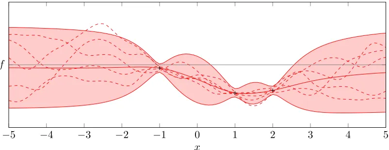
−5 −4 −3 −2 −1 0 1 2 3 4 5 f

x

Figure 1: A Gaussian process measure (rational quadratic kernel), conditioned on three previous observations (black crosses). Mean function in solid red, marginal standard deviation at each location (two standard deviations) as light red tube. Five sampled functions from the current belief as dashed red lines. Arbitrary ordinate scale, zero in gray.

predicting change to pmin The Gaussian process measure affords a straightforward but rarely used

analytic probabilistic formulation for thechangeofp(f)as a function of the next evaluation point (Section 2.4).

choosing loss function We commit to relativeentropyfrom a uniform distribution as the loss func-tion, as this can be interpreted as a utility on gained information about the location of the minimum (Section 2.5).

predicting expected information gain From the predicted change, we construct a first-order ex-pansion on_h

L

_ifrom future evaluations and, again, compare to the asymptotically exact Monte Carlo answer (Section 2.6).

choosing greedily Faced with the exponential cost of the exact dynamic problem to the horizonH, we accept a greedy approach for the reduction of_h

L

_iat every step. We illustrate the effect of this shortcut in an example setting (Section 2.7).

2.1 Gaussian Process Measure on f

The remainder of the paper commits to Gaussian process measures for p(f). These are conve-nient for the task at hand due to their descriptive generality and their conveconve-nient analytic properties. Since this paper is aimed at readers from several communities, this section contains a very brief introduction to some relevant aspects of Gaussian processes; readers familiar with the subject can safely skip ahead. A thorough introduction can be found in a textbook of Rasmussen and Williams (2006). Some readers from other fields may find it helpful to know that more or less special cases of Gaussian process inference are elsewhere known under names like Kriging(Krige, 1951) and

should not be assumed to carry over to Gaussian process inference as understood in machine learn-ing.

A Gaussian process is an indimensional probability density, such that each linear finite-dimensional restriction is multivariate Gaussian. The infinite-finite-dimensional space can be thought of as a space of functions, and the finite-dimensional restrictions asvalues of those functions at locations_{x∗_i}i=1,...,N. Gaussian process beliefs are parametrized by amean function m:I_Rand acovariance function k:I_×I_{_}R_{. For our particular analysis, we restrict the domainI to finite,}

compact subsets of the real vector spacesRD_{. The covariance function, also known as thekernel, has}

to be positive definite, in the sense that any finite-dimensional matrix with elementsKi j=k(xi,xj)

has to be positive definite_∀xi,xj∈I. A number of such kernel functions are known in the literature,

and different kernel functions induce different kinds of Gaussian process measures over the space of functions. Among the most widely used kernels for regression are thesquared exponentialkernel

kSE(x,x′;S,s) =s2exp

−1₂(x₋x′)⊺_S−1_(x −x′)

,

which induces a measure that puts nonzero mass on only smooth functions ofcharacteristic length-scale Sandsignal variance s2(MacKay, 1998b), and therational quadratickernel (Mat´ern, 1960; Rasmussen and Williams, 2006)

kRQ(x,x′;S,s,α) =s2

1+ 1

2α(x−x

′₎⊺_S−1_(x −x′)

−α ,

which induces a belief over smooth functions whose characteristic length scales are a scale mix-ture over a distribution of width 1/α and locationS. Other kernels can be used to induce beliefs over non-smooth functions (Mat´ern, 1960), and even over non-continuous functions (Uhlenbeck and Ornstein, 1930). Experiments in this paper use the two kernels defined above, but the results apply to all kernels inducing beliefs over continuousfunctions. While there is a straightforward relationship between kernel continuity and the mean square continuity of the inducedprocess, the relationship between the kernel function and the continuity of each sample is considerably more involved (Adler, 1981, §3). Regularity of the kernel also plays a nontrivial role in the question whether the distribution of infima of samples from the process is well-defined at all (Adler, 1990). In this work, we side-step this issue by assuming that the chosen kernel is sufficiently regular to induce a well-defined belief pminas defined by Equation (8).

Kernels form a semiring: products and sums of kernels are kernels. These operations can be used to generalize the induced beliefs over the function space (Section 2.8.3). Without loss of generality, the mean function is often set tom_≡0 in theoretical analyses, and this paper will keep with this tradition, except for Section 2.8.3. Where mis nonzero, its effect is a straightforward off-set p(f(x))_p(f(x)−m(x)).

For the purpose of regression, the most important aspect of Gaussian process priors is that they are conjugate to the likelihood from finitely many observations(X,Y) =_{xi,yi}i=1,...,N of the form

yi(xi) = f(xi) +ξwith Gaussian noiseξ∼

N

(0,σ2). The posterior is a Gaussian process with mean

and covariance functions

µ(x∗) =kx∗_,X[K_X,X+σ2I]−1y ; Σ(x∗,x_∗) =k_x∗_,x∗−k_x∗_,X[K_X,X+σ2I]−1k_X,x∗, (3) whereKX,X is the kernel Gram matrixK_X(i_,,_Xj)=k(xi,xj), and other objects of the formka,b are also

−5 −4 −3 −2 −1 0 1 2 3 4 5 f

x

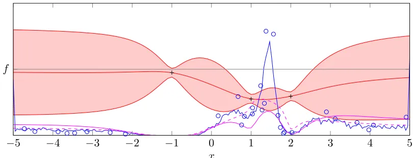
Figure 2: pmininduced byp(f)from Figure 1. p(f)repeated for reference. Blue solid line:

Asymp-totically exact representation ofpmingained from exact sampling of functions on a regular

grid (artifacts due to finite sample size). For comparison, the plot also shows the local utilitiesprobability of improvement(dashed magenta) and expected improvement(solid magenta) often used for Gaussian process global optimization. Blue circles: Approximate representation on representer points, sampled from probability of improvement measure. Stochastic error on sampled values, due to only asymptotically correct assignment of mass to samples, and varying density of points, focusing on relevant areas of pmin. This

plot uses arbitrary scales for each object: The two heuristics have different units of mea-sure, differing from that ofpmin. Notice the interesting features ofpminat the boundaries

of the domain: The prior belief encodes that f is smooth, and puts finite probability mass on the hypothesis that f has negative (positive) derivative at the right (left) boundary of the domain. With nonzero probability, the minimum thus lies exactly on the boundary of the domain, rather than within a Taylor radius of it.

it is straightforward to sample “functions” (point-sets of arbitrary size from I) from a Gaussian process. To sample the value of a particular sample at the M locations X∗, evaluate mean and variance function as a function of any previously collected data points, using Equation (3), draw a vector ζ_∼∏M

N

(0,1)ofM random numbers i.i.d. from a standard one-dimensional Gaussian distribution, then evaluate

˜

f(X∗) =µ(X∗) +C_[Σ(X∗_,X∗_)]⊺_ζ,

where the operatorC_{denotes the Cholesky decomposition (Benoit, 1924).}

2.2 Discrete Representations for Continuous Distributions

Having established a probability measure p(f)on the function, we turn to constructing the belief

pmin(x)over its minimum. Inspecting Equation (1), it becomes apparent that it is challenging in two

It may seem daunting thatpmininvolves an infinite-dimensional integral. The crucial observation

for a meaningful approximation in finite time is that regular functions can be represented meaning-fully on finitely many points. If the stochastic process representing the belief over f is sufficiently regular, then Equation (1) can be approximated arbitrarily well with finitely many representer points. The discretization grid need not be regular—it may be sampled from any distribution which puts non-zero measure on every open neighborhood ofI. This latter point is central to a graceful han-dling of the curse of dimensionality: The na¨ıve approach of approximately solving Equation (1) on a regular grid, in aD-dimensional domain, would require

O

(exp(D))points to achieve any given resolution. This is obviously not efficient: Just like in other numerical quadrature problems, any given resolution can be achieved with fewer representer points if they are chosen irregularly, with higher resolution in regions of greater influence on the result of integration. We thus choose to

samplerepresenter points from a proposal measureu, using a Markov chain Monte Carlo sampler (our implementation uses shrinking rank slice sampling, by Thompson and Neal, 2010).

What is the effect of this stochastic discretization? A non-uniform quadrature measure u(x)˜ for N representer locations _{x˜i}i=1,...,N leads to varying widths in the “steps” of the representing

staircase function. AsN_{_}∞, the width of each step is approximately proportional to(u(x˜i)N)−1.

Section 2.3 will construct a discretized ˆqmin(x˜i)that is an approximation to the probability that fmin

occurs within the step at ˜xi. So the approximate ˆpminon this step is proportional to ˆqmin(x˜i)u(x˜i),

and can be easily normalized numerically, to become an approximation topmin.

How should the measure u be chosen? Unfortunately, the result of the integration, being a density rather than a function, is itself a function of u, and the loss-function is also part of the problem. So it is nontrivial to construct an optimal quadrature measure. Intuitively, a good proposal measure for discretization points should put high resolution on regions ofI where the shape ofpmin

has strong influence on the loss, and on its change. For our choice of loss function (Section 2.5), it is a good idea to chooseusuch that it puts high mass on regions of high value for pmin. But for

other functions, this need not always be the case.

We have experimented with a number of ad hoc choices foru, and found the aforementioned “expected improvement” and “probability of improvement” (Section 1.1.3) to lead to reasonably good performance. We use these functions for a similar reason as their original authors: Because they tend to have high value in regions where pmin is also large. To avoid confusion, however,

note that we use these functions as unnormalized measures tosample discretization pointsfor our

calculationofpmin, not as an approximation forpminitself, as was done in previous work by other

authors. Defects in these heuristics have weaker effect on our algorithm than in the cited works: in our case, ifu is not a good proposal measure, we simply need more samples to construct a good representation of pmin. In the limit ofN_∞, all choices ofuperform equally well, as long as they put nonzero mass on all open neighborhoods of the domain.

2.3 Approximating pminwith Expectation Propagation

The previous Section 2.2 provided a way to construct a non-uniform grid ofN discrete locations ˜

xi, i=1, . . . ,N. The restriction of the Gaussian process belief to these locations is a multivariate

Gaussian density with mean ˜µ_∈RN_{and covariance ˜Σ∈}RN×N_{. So Equation (1) reduces to a discrete}

probabilitydistribution(as opposed to a density)

ˆ

pmin(xi) =

Z

f∈RN

N

(f; ˜µ,Σ˜)

N

∏

i6=j

f

N

(f; ˜µ,Σ˜) θ[f(x˜j)−f(x˜i)]

i₆= j

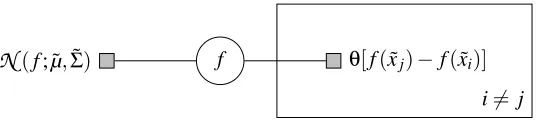
Figure 3: Graphical model providing motivation for EP approximation onpmin. See text for details.

This is a multivariate Gaussian integral over a half-open, convex, piecewise linearly constrained integration region—a polyhedral cone. Unfortunately, such integrals are known to be intractable (Plackett, 1954; Lazard-Holly and Holly, 2003). However, it is possible to construct an effective approximation ˆqmin based on Expectation Propagation (EP) (Minka, 2001): Consider the belief p(f(x))˜ as a “prior message” on f(x)˜ , and each of the terms in the product as one factor providing another message. This gives the graphical model shown in Figure 3. Running EP on this graph provides an approximate Gaussian marginal, whose normalization constant ˆqmin(xi), which EP also

provides, approximates p(f_|xmin=xi). The EP algorithm itself is somewhat involved, and there

are a number of algorithmic technicalities to take into account for this particular setting. We refer interested readers to recent work by Cunningham et al. (2011), which gives a detailed description of these aspects. The cited work also establishes that, while EP’s approximations to Gaussian integrals are not always reliable, in this particular case, where there are as many constraints as dimensions to the problem, the approximation is generally of high quality (see Figure 4 for an example). An important advantage of the EP approximation over both numerical integration and Monte Carlo integration (see next Section) is that it allows analytic differentiation of ˆqmin with respect to the

parameters ˜µand ˜Σ(Cunningham et al., 2011; Seeger, 2008). This fact will become important in Section 2.6.

The computational cost of this approximation is considerable: Each computation of ˆqmin(x˜i), for

a giveni, involvesN factor updates, which each have rank 1 and thus cost

O

(N2_{). So, overall, the}

cost of calculating ˆqmin(˜x)is

O

(N4). This meansNis effectively limited to well belowN=1000.

Our implementation uses a default of N=50, and can calculate next evaluation points in_∼10 seconds. Once again, it is clear that this algorithm is not suitable for simple numerical optimization problems; but a few seconds are arguably an acceptable waiting time for physical optimization problems.

2.3.1 AN ALTERNATIVE: SAMPLING

An alternative to EP is Monte Carlo integration: sample S functions exactly from the Gaussian belief on p(f), at costO(N2_{) per sample, then find the minimum for each sample in}

_O

_{(N) time.}

This technique was used to generate the asymptotically exact plots in Figures 2 and following. It has overall cost

O

(SN3_{), and can be implemented efficiently using Matrix-Matrix multiplications,}

−5 −4 −3 −2 −1 0 1 2 3 4 5 f

x

Figure 4: EP-approximation topmin(dashed green). Other plots as in previous figures. EP achieves

good agreement with the asymptotically exact Monte Carlo approximation to pmin,

in-cluding the point masses at the boundaries of the domain.

Figure 5: Innovation from two observations atx=₋3 andx=3. Current belief as red outline in background, from Figure 1. Samples from the belief over possible beliefs after observa-tions atxin blue. For each sampled innovation, the plot also shows the induced innovated

pmin(lower sampling resolution as previous plots). Innovations from several (here: two)

observations can be sampled jointly.

2.4 Predicting Innovation from Future Observations

As detailed in Equation (2), the optimal choice of the nextH evaluations is such that theexpected

change in the loss_h

L

_ixis extremal, that is, it effects the biggest possible expected drop in loss. The

loss is a function ofpmin, which in turn is a function ofp(f). So predicting change in loss requires

predicting change in p(f) as a function of the next evaluation points. It is another convenient aspect of Gaussian processes that they allow such predictions in analytic form (Hennig, 2011): Let previous observations atX0have yielded observationsY0. Evaluating at locationsX will give new

observationsY, and the mean will be given by

µ(x∗) = [kx∗_,X0,k_x∗_,X]

KX0,X0 kX0,X kX,X0 KX,X

−1 Y0

Y

=kx∗_,X0K_X−_0,1_X

0Y0+ (kx∗,X−kx∗,X0K− 1

X0,X0kX0,X)× (kX,X−kX,X0K−

1

X0,X0kX0,X)

−1_(Y−k X,X0K−

1 X0,X0Y0) =µ0(x∗) +Σ0(x∗,X)Σ−01(X,X)(Y−µ0(X)),

(4)

whereK_a(i_,,_bj)=k(ai,bj) +δi jσ2. The step from the first to the second line involves an application of

the matrix inversion lemma, the last line uses the mean and covariance functions conditioned on the data set(X0,Y0)so far. SinceY is presumed to come from this very Gaussian process belief, we

can write

Y =µ(X) +C_[Σ(X,X)]⊺_Ω′_{+σω=µ(X) +C[Σ(X,X) +σ}2_I

H]⊺Ω Ω,Ω′,ω∼

N

(0,IH),

and Equation (4) simplifies. An even simpler construction can be made for the covariance function. We find that mean and covariance function of the posterior after observations(X,Y)are mean and covariance function of the prior, incremented by theinnovations

∆µX,Ω(x∗) =Σ(x∗,X)Σ−1(X,X)C[Σ(X,X) +σ2IH]Ω

∆ΣX(x∗,x∗) =Σ(x∗,X)Σ−1(X,X)Σ(X,x∗).

The change to the mean function is stochastic, while the change to the covariance function is deter-ministic. Both innovations are functions both ofX and of the evaluation pointsx∗. One use of this result is to sample_h

L

_iX by sampling innovations, then evaluating the innovatedpminfor each

inno-vation in an inner loop, as described in Section 2.3.1. An alternative, described in the next section, is to construct an analytic first order approximation to_h

L

_iX from the EP prediction constructed in Section 2.3. As mentioned above, the advantage of this latter option is that it provides an analytic function, with derivatives, which allows efficient numerical local optimization.

2.5 Information Gain—the Log Loss

To solve the decision problem of where to evaluate the function next in order to learn most about the location of the minimum, we need to say what it means to “learn”. Thus, we require a loss functional that evaluates the information content of innovated beliefs pmin. This is, of course, a

core idea in information theory. The seminal paper by Shannon (1948) showed that the negative expectation of probability logarithms,

H_{[p] =−hlogpip=−}

∑

i

−5 −4 −3 −2 −1 0 1 2 3 4 5 f

x

Figure 6: 1-step predicted loss improvement for the log loss (relative entropy). Upper part of plot as before, for reference. Monte Carlo prediction on regular grid as solid black line. Monte Carlo prediction from sampled irregular grid as dot-dashed black line. EP prediction on regular grid as black dashed line. EP prediction from samples as black dotted line. The minima of these functions, where the algorithm will evaluate next, are marked by vertical lines. While the predictions from the various approximations are not identical, they lead to similar next evaluation points. Note that these next evaluation points differ qualitatively from the choice of the GP optimization heuristics of Figure 2. Since each approximation is only tractable up a multiplicative constant, the scales of these plots are arbitrary, and only chosen to overlap for convenience.

known as entropy, has a number of properties that allow its interpretation as a measure of uncer-tainty represented by a probability distribution p. Its value can be be interpreted as the number of natural information units an optimal compression algorithm requires to encode a sample from the distribution, given knowledge of the distribution. However, it has since been pointed out repeatedly that this concept does not easily generalize to probability densities. A density p(x) has a unit of measure[x]−1_{, so its logarithm is not well-defined, and one cannot simply replace summation with}

integration in Equation (5). A functional thatiswell-defined on probability densities and preserves many of the information-content interpretations of entropy (Jaynes and Bretthorst, 2003) isrelative entropy, also known as Kullback-Leibler (1951) divergence. We use its negative value as a loss function for information gain.

L

_KL(p;b) =₋ Z

p(x)logp(x)

b(x)dx.

As base measure b we choose the uniform measureU_{I(x) =|I|}−1 _{over I, which is well-defined}

becauseI is presumed to be bounded.2 With this choice, the loss is maximized (at

L

=0) for a

uniform belief over the minimum, and diverges toward negative infinity if p approaches a Dirac point distribution. The resulting algorithm, Entropy Search, will thus choose evaluation points such that it expects to move away from the uniform base measure toward a Dirac distribution as quickly as possible.

The reader may wonder: What about the alternative idea of maximizing, at each evaluation, entropy relative to thecurrent pmin? This would only encourage the algorithm to attempt to change

the current belief, but not necessarily in the right direction. For example, if the current belief puts very low mass on a certain region, an evaluation that has even a small chance of increasing pmin

in this region could appear more favorable than an alternative evaluation predicted to have a large effect on regions where the current pminhas larger values. The point is not to just changepmin, but

to change it such that it moves away from the base measure.

Recall that we approximate thedensity p(x)using adistributionp(xˆ i)on a finite set{xi}of

rep-resenter points, which define steps of width proportional, up to stochastic error, to an unnormalized measure ˜u(xi). In other words, we can approximate pmin(x)as

pmin(x)≈

ˆ

p(xi)Nu(x˜ i)

Zu

; Zu=

Z

˜

u(x)dx; xi=arg min {xj}

kx₋xjk.

We also note that afterN samples, the unit element of measure has size, up to stochastic error, of

∆xi≈_u˜(Z_xiu_)N. So we can approximately represent the loss

L

_KL(pmin;b) ≈ −∑ipmin(xi)∆xilogpmin_b(x(_ix₎i)

=₋∑ipˆmin(xi)logpˆmin_Z(_ux_bi)₍N_xiu₎˜(xi)

=₋∑ipˆmin(xi)logpˆmin_b(₍x_xi)_iu₎˜(xi)+log Z_Nu

∑ipˆmin(xi)

=H_{[pˆmin]− hlog ˜uipˆ}

min+hlogbipˆmin+logZu−logN,

which means we do not require the normalization constant Zu for optimization of

L

KL. For our

uniform base measure, the third term in the last line is a constant, too; but other base measures would contribute nontrivially.

2.6 First-Order Approximation to_h

L

_i

Since EP provides analytic derivatives of pmin with respect to mean and covariance of the

Gaus-sian measure over f, we can construct a first order expansion of the expected change in loss from evaluations. To do so, we consider, in turn, the effect of evaluations atX on the measure on f, the induced change in pmin, and finally the change in

L. Since the change to the mean is Gaussian

stochastic, It¯o’s (1951) Lemma applies. The following Equation uses the summation convention: double indices in products are summed over.

h∆

L

_iX = Z

L

p0_min+ ∂pmin

∂Σ(x˜i,x˜j)

∆ΣX(x˜i,x˜j) +

∂2_p min

∂µi∂µj

∆µX,1(x˜i)∆µX,1(x˜j)

+∂pmin

∂µ(x˜i)

∆X,Ωµ(x˜i) +

O

((∆µ)2,(∆Σ)2)

N

(Ω; 0,1)dΩ₋

L

[p0

min]. (6) uniform. For example, uniform measures on the [0,1] simplex appear bell-shaped in the softmax basis (MacKay, 1998a). So, whilebhere does not represent prior knowledge onxmin per se, it does provide a unit of measure to

−4 −2 0 2 4 −4

−2

0

2

4

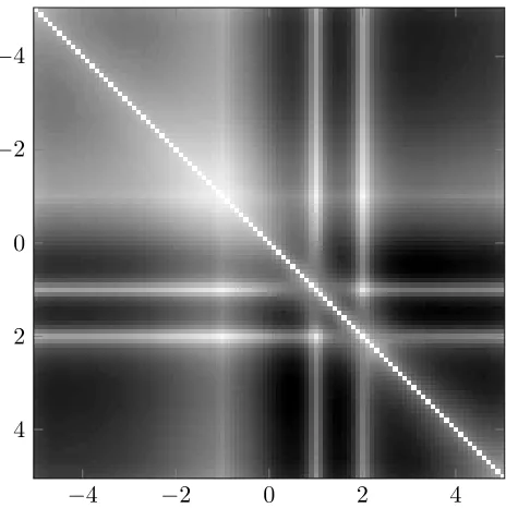
Figure 7: Expected drop in relative entropy (see Section 2.5) from two additional evaluations to the three old evaluations shown in previous plots. First new evaluation on abscissa, second new evaluation on ordinate, but due to the exchangeability of Gaussian process measures, the plot is symmetric. Diagonal elements excluded for numerical reasons. Blue regions are more beneficial than red ones. The relatively complicated structure of this plot illus-trates the complexity of finding the optimalH-step evaluation locations.

The first line contains deterministic effects, the first term in the second line covers the stochastic aspect. Monte Carlo integration over the stochastic effects can be performed approximately using a small number of samplesΩ. These samples should be drawn only once, at first calculation, to get a differentiable function_h∆

L

_iX that can be re-used in subsequent optimization steps.

The above formulation is agnostic with respect to the loss function. Hence, in principle, Entropy Search should be easy to generalize to different loss functions. But recall that the fidelity of the calculation of Equation (6) depends on the intermediate approximate steps, in particular the choice of discretization measure ˜u. We have experimented with other loss functions and found it difficult to find a good measure ˜uproviding good performance for many such loss functions. So this paper is limited to the specific choice of the relative entropy loss function. Generalization to other losses is future work.

2.7 Greedy Planning, and its Defects

The previous sections constructed a means to predict, approximately, the expected drop in loss from

Hnew evaluations at locationsX=_{xi}i=1,...,N. The remaining task is to optimize these locations.

function numerically, without noise, with derivatives, and at hopefully relatively low cost compared to the physical process we are ultimately trying to optimize.

Nevertheless, one issue remains: Optimizing evaluations over the entire horizonHis a dynamic programming problem, which, in general, has cost exponential inH. However, this problem has a particular structure: Apart from the fact that evaluations drawn from Gaussian process measures are exchangeable, there is also other evidence that optimization problems are benign from the point of view of planning. For example, Srinivas et al. (2010) show that the information gain over the func-tion values is submodular, so that greedy learning of the funcfunc-tion comes close to optimal learning of the function. While is is not immediately clear whether this statement extends to our issue of learning about the function’s minimum, it is obvious that the greedy choice of whatever evaluation location most reduces expected loss in the immediate next step is guaranteed to never be catastroph-ically wrong. In contrast to general planning, there are no “dead ends” in inference problems. At worst, a greedy algorithm may choose an evaluation point revealed as redundant by a later step. But thanks to the consistency of Bayesian inference in general, and Gaussian process priors in particular (van der Vaart and van Zanten, 2011), no decision can lead to an evaluation that somehow makes it impossible to learn the true function afterward. In our approximate algorithm, we thus adopt this greedy approach. It remains an open question for future research whether approximate planning techniques can be applied efficiently to improve performance in this planning problem.

2.8 Further Issues

This section digresses from the main line of thought to briefly touch upon some extensions and issues arising from the choices made in previous sections. For the most part, we point out well-known analytic properties and approximations that can be used to generalize the algorithm. Since they apply to Gaussian process regression rather than the optimizer itself, they will not play a role in the empirical evaluation of Section 3.

2.8.1 DERIVATIVEOBSERVATIONS

Gaussian process inference remains analytically tractable if instead of, or in addition to direct obser-vations of f, we observe the result of anylinearoperator acting on f. This includes observations of the function’s derivatives (Rasmussen and Williams, 2006, §9.4) and, with some caveats, to integral observations (Minka, 2000). The extension is pleasingly straightforward: The kernel defines co-variances between function values. Coco-variances between the function and its derivatives are simply given by

cov ∂

n_f(x)

∏i∂xi ,∂

m_f(x′₎

∏j∂x′j !

= ∂

n+m_k(x,x′₎

∏i∂xi∏j∂x′j ,

−2 0 2

−10

−5

0 5 10

x

f

(

x

)

base kernel poly lik

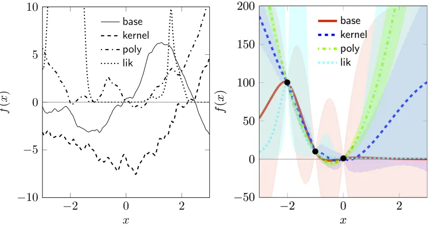
Figure 8: Generalizing GP regression. Left: Samples from different priors. Right: Posteriors (mean, two standard deviations) after observing three data points with negligible noise (kernel parameters differ between the two plots). base: standard GP regression with Mat´ern kernel. kernel: sum of two kernels (square exponential and rational quadratic) of different length scales and strengths. poly: polynomial (here: quadratic) mean function.

lik: Non-Gaussian likelihood (here: logarithmic link function). The scales of bothxand

f(x)are functions of kernel parameters, so the numerical values in this plot have relevance only relative to each other. Note the strong differences in both mean and covariance functions of the posteriors.

2.8.2 LEARNINGHYPERPARAMETERS

Throughout this paper, we have assumed kernel and likelihood function to be given. In real appli-cations, this will not usually be the case. In such situations, the hyperparameters defining these two functions, and if necessary a mean function, can be learned from the data, either by setting them to maximum likelihood values, or by full-scale Bayesian inference using Markov chain Monte Carlo methods. See Rasmussen and Williams (2006, §5) and Murray and Adams (2010) for details. In the latter case, the beliefp(f)over the function is a mixture of Gaussian processes. To still be able to use the algorithm derived so far, we approximate this belief with a single Gaussian process by calculating expected values of mean and covariance function.

2.8.3 LIMITATIONS ANDEXTENSIONS OFGAUSSIANPROCESSES FOROPTIMIZATION

Like any probability measure over functions, Gaussian process measures are not arbitrarily general. In particular, the most widely used kernels, including the two mentioned above, are stationary, meaning they only depend on the difference between locations, not their absolute values. Loosely speaking, the prior “looks the same everywhere”. One may argue that many real optimization problems do not have this structure. For example, it may be known that the function tends to have larger functions values toward the boundaries ofIor, more vaguely, that it is roughly “bowl-shaped”. Fortunately, a number of extensions readily suggest themselves to address such issues (Figure 8).

Parametric Means As pointed out in Section 2.1, we are free to add any parametric general linear model as the mean function of the Gaussian process,

m(x) =

_∑

i

φi(x)wi.

Using Gaussian beliefs on the weightswiof this model, this model may be learned at the same

time as the Gaussian process itself (Rasmussen and Williams, 2006, §2.7). Polynomials such as the quadraticφ(x) = [x;xx⊺_{]are beguiling in this regard, but they create an explicit “origin”}

at the center ofI, and induce strong long-range correlations between opposite ends ofI. This seems pathological: In most settings, observing the function on one end ofIshould not tell us much about the value at the opposite end ofI. But we may more generally choose any feature set for the linear model. For example, a set of radial basis functionsφi(x) =exp(kx−cik2/ℓ2i)

around locationsci at the rims of I can explain large function values in a region of widthℓi

around such a feature, without having to predict large values at the center ofI. This idea can be extended to a nonparametric version, described in the next point.

Composite Kernels Since kernels form a semiring, we may sum a kernel of large length scale and large signal variance and a kernel of short length scale and low signal variance. For example

k(x,x′) =kSE(x,x′;s1,S1) +kRQ(x,x′,s2,S2,α2) s1≫s2;Si j₁ ≫Si j₂ ∀i,j

yields a kernel over functions that, within the bounded domainI, look like “rough troughs”: global curvature paired with local stationary variations. A disadvantage of this prior is that it thinks “domes” just as likely as “bowls”. An advantage is that it is a very flexible framework, and does not induce unwanted global correlations.

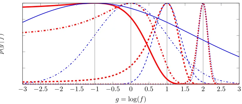
Nonlinear Likelihoods An altogether different effect can be achieved by a Gaussian, non-linear likelihood function. For example, if f is known to be strictly positive, one may assume the noise model

p(y_|g) =

N

(y; exp(g),σ2_{); f =exp(g), (7)}

and learnginstead of f. Since the logarithm is a convex function, the minimum of the la-tentg is also a minium of f. Of course, this likelihood leads to a non-Gaussian posterior. To retain a tractable algorithm, approximate inference methods can be used to construct ap-proximate Gaussian posteriors. In our example (labeledlik_{in Figure 8), we used a Laplace}

approximation: It is straightforward to show that Equation (7) implies

∂logp(y_|g)

∂g

g=gˆ !

=0 _⇒gˆ=logy ∂

2_logp(y|g)

∂2_g

g=gˆ = y

2

−3 −2.5 −2 −1.5 −1 −0.5 0 0.5 1 1.5 2 2.5 3

g= log(f)

p

(

y

|

f

)

Figure 9: Laplace approximation for a logarithmic Gaussian likelihood. True likelihood in thick red, Gaussian approximation in thin blue, maximum likelihood solution marked in grey. Four log relative valuesa=log(y/σ)of sampleyand noiseσ(scaled in height for read-ability).a=₋1 (solid);a=0 (dash-dotted);a=1 (dashed);a=2 (dotted). The approx-imation is good fora_≫0.

so a Laplace approximation amounts to a heteroscedastic noise model, in which an observa-tion(y,σ2_{)is incorporated into the Gaussian process as(log(y),(σ/y)}2_{). This approximation}

is valid ifσ_≪y(see Figure 9). For functions on logarithmic scales, however, finding min-ima smaller than the noise level, at logarithmic resolution, is a considerably harder problem anyway.

The right part of Figure 8 shows posteriors produced using the three approaches detailed above, and the base case of a single kernel with strong signal variance, when presented with the same three data points, with very low noise. The strong difference between the posteriors may be disappointing, but it is a fundamental aspect of inference: Different prior assumptions lead to different posteriors, and function space inference is impossible without priors. Each of the four beliefs shown in the Figure may be preferable over the others in particular situations. The polynomial mean describes functions that are almost parabolic. The exponential likelihood approximation is appropriate for functions with an intrinsic logarithmic scale. The sum kernel approach is pertinent for the search for local minima of globally stationary functions. Classic methods based on polynomial approximations are a lot more restrictive than any of the models described above.

Perhaps the most general option is to use additional prior information

I

givingp(xmin|

I

),

inde-pendent ofp(f), to encode outside information about the location of the minimum. Unfortunately, this is intractable in general. But it may be approached through approximations. This option is outside of the scope of this paper, but will be the subject of future work.

2.9 Summary—the Entire Algorithm

Algorithm 1Entropy Search

1: procedureENTROPYSEARCH(k,l=p(y_|f(x)),u,H,(x,y))

2: x˜_∼u(x,y) ⊲discretize using measureu(Section 2.2) 3: [µ,Σ,∆µ_x,∆Σx]^GP(k,l,x,y) ⊲infer function, innovation, from GP prior (2.1)

4: [qˆmin(x)˜ ,∂ˆq_∂min_µ ,∂ 2_qˆ

min ∂µ∂µ ,

∂qˆminx

∂Σ ]^EP(µ,Σ) ⊲approximate ˆpmin(2.3)

5: ifH=0then

6: returnqmin ⊲At horizon, return belief for final decision

7: else

8: x′_^arg min_h

L

_ix ⊲predict information gain; Equation (6)

9: y′^EVALUATE(f(x′)) ⊲take measurement 10: ENTROPYSEARCH(k,l,u,H₋1,(x,y)_∪(x′,y′)) ⊲move to next evaluation 11: end if

12: end procedure

be a function of previous data, the HorizonH, and any previously collected observations(x,y). To choose where to evaluate next, we first sample discretization points fromu, then calculate the current Gaussian belief over fon the discretized domain, along with its derivatives. We construct an approx-imation to the belief over the minimum using Expectation Propagation, again with derivatives. Fi-nally, we construct a first order approximation on the expected information gain from an evaluation atx′and optimize numerically. We evaluate f at this location, then the cycle repeats. An example implementation inMATLABcan be downloaded fromwww.probabilistic-optimization.org.

3. Experiments

Figures in previous sections provided some intuition and anecdotal evidence for the efficacy of the various approximations used by Entropy Search. In this section, we compare the resulting algorithm to two Gaussian process global optimization heuristics: Expected Improvement, Probability of Im-provement (Section 1.1.3), as well as to a continuous armed bandit algorithm: GP-UCB (Srinivas et al., 2010). For reference, we also compare to a number of numerical optimization algorithms: Trust-Region-Reflective (Coleman and Li, 1996, 1994), Active-Set (Powell, 1978b,a), interior point (Byrd et al., 1999, 2000; Waltz et al., 2006), and a na¨ıvely projected version of the BFGS algorithm (Broyden, 1965; Fletcher, 1970; Goldfarb, 1970; Shanno, 1970). We avoid implementation bias by using a uniform code framework for the three Gaussian process-based algorithms, that is, the algo-rithms share code for the Gaussian process inference and only differ in the way they calculate their utility. For the local numerical algorithms, we used third party code: The projected BFGS method is based on code by Carl Rasmussen,3the other methods come from version 6.0 of the optimization toolbox ofMATLAB.4

In some communities, optimization algorithms are tested on hand-crafted test functions. This runs the risk of introducing bias. Instead, we compare our algorithms on a number of functions sampled from a generative model. In the first experiment, the function is sampled from the model used by the GP algorithms themselves. This eliminates all model-mismatch issues and allows a

3. Code can be found athttp://www.gaussianprocess.org/gpml/code/matlab/util/minimize.m, version using BFGS: personal communication.

0 10 20 30 40 50 60 70 80 90 100 10−5

10−4

10−3

10−2

10−1

100 101

# of evaluations

|

fmin

−

ˆ_fmin

|

trust region reflective active set

interior point BFGS GP UCB

prob. of improvement expected improvement entropy search

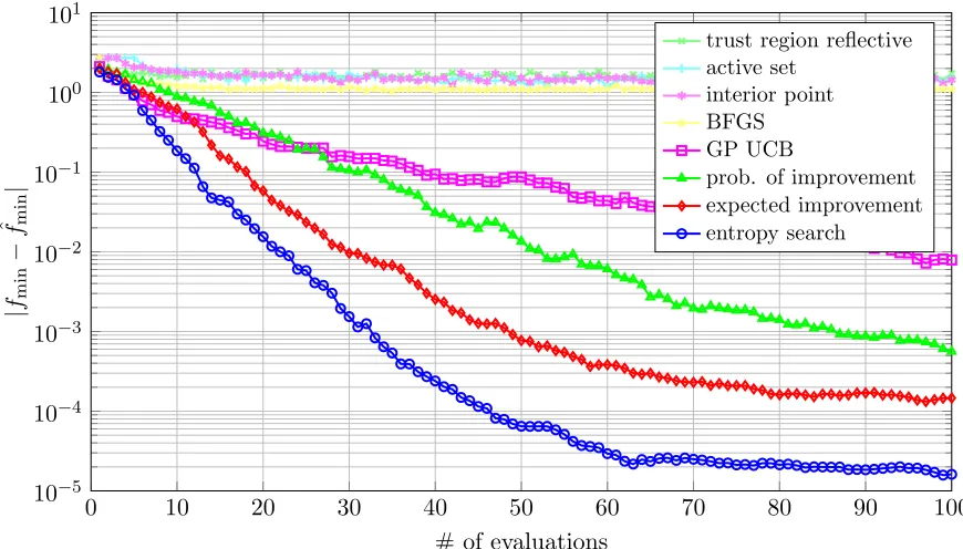
Figure 10: Distance of function value at optimizers’ best guess forxminfrom true global minimum.

Log scale.

direct comparison of other GP optimizers to the probabilistic optimizer. In a second experiment, the functions were sampled from a model strictly more general than the model used by the algorithms, to show the effect of model mismatch.

3.1 Within-Model Comparison

The first experiment was carried out over the 2-dimensional unit domainI = [0,1]2_{. To generate}

test functions, 1000 function values were jointly sampled from a Gaussian process with a squared-exponential covariance function of length scaleℓ=0.1 in each direction and unit signal variance. The resulting posterior mean was used as the test function. All algorithms had access to noisy eval-uations of the test functions. For the benefit of the numerical optimizers, noise was kept relatively low: Gaussian with standard deviationσ=10−3. All algorithms were tested on the same set of 40 test functions, all Figures in this section are averages over those sets of functions. It is nontrivial to provide error bars on these average estimates, because the data sets have no parametric distribution. But the regular structure of the plots, given that individual experiments were drawn i.i.d., indicates that there is little remaining stochastic error.

After each function evaluation, the algorithms were asked to return a best guess for the minimum

xmin. For the local algorithms, this is simply the point of their next evaluation. The Gaussian process

0 10 20 30 40 50 60 70 80 90 100 10−4

10−3

10−2

10−1

100

# of evaluations

|

x

min

−

ˆ

x

min

|

trust region reflective active set

interior point BFGS GP UCB

prob. of improvement expected improvement entropy search

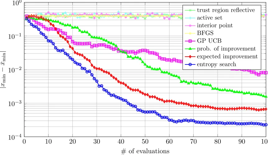
Figure 11: Euclidean distance of optimizers’ best guess forxminfrom truth. Log scale.

in general lie at a data point, their quality can actually decrease during optimization. The most obvious feature of this plot is that local optimization algorithms are not adept at finding global minima, which is not surprising, but gives an intuition for the difficulty of problems sampled from this generative model. The plot shows a clear advantage for Entropy Search over its competitors, even though the algorithm does not directly aim to optimize this particular loss function. The flattening out of the error of all three global optimizers toward the right is due to evaluation noise (recall that evaluations include Gaussian noise of standard deviation 10−3). Interestingly, Entropy Search flattens out at an error almost an order of magnitude lower than that of the nearest competitor, Expected Improvement. One possible explanation for this behavior is a pathology in the classic heuristics: Both Expected Improvement and Probability of Improvement require a “current best guess”η, which has to be a point estimate, because proper marginalization over an uncertain belief is not tractable. Due to noise, it can thus happen that this best guess is overly optimistic, and the algorithm then explores too aggressively in later stages.

Figure 11 shows data from the same experiments as the previous figure, but plots Euclidean distance from the true global optimum in input space, rather than in function value space. The results from this view are qualitatively similar to those shown in Figure 10.

0 10 20 30 40 50 60 70 80 90 100 0

50 100 150 200 250 300

# of evaluations

regret

GP UCB

prob. of improvement expected improvement entropy search

Figure 12: Regret as a function of number of evaluations.

We pointed out in Section 1.1.2 that the bandit setting differs considerably from the kind of optimization discussed in this paper, because bandit algorithms try to minimize regret, rather than improve an estimate of the function’s optimum. To clarify this point further, Figure 12 shows the regret

r(T) =

T

∑

t=1

[yt−fmin],

for each of the algorithms. Notice that probability of improvement, which performs worst among the global algorithms as seen from the previous two measures of performance, achieves the lowest regret. The intuition here is that this heuristic focuses evaluations on regions known to give low function values. In contrast, the actual value of the functionat the evaluation pointhas no special role in Entropy Search. The utility of an evaluation point only depends on its expected effect on knowledge about the minimum of the function.

Surprisingly, the one algorithm explicitly designed to achieve low regret, GP-UCB, performs worst in this comparison. This algorithm chooses evaluation points according to (Srinivas et al., 2010)

xnext=arg min x

[µ(x)₋β1/2σ(x)] where β=4(D+1)logT+C(k,δ)

0 0

.2 0.4 0.6 0.8 1

0

0_.2

0

.4

0

.6

0_.8

1

−2 0 2

0 0

.2 0.4 0.6 0.8 1

0

0_.2

0

.4

0

.6

0_.8

1

−1

0 1 2 3

Figure 13: Left:A sample from the GP prior with squared exponential kernel used in the on-model experiments of Section 3.1.Right:Sample from prior with the rational quadratic kernel used for the out-of-model comparison of Section 3.2.

3.2 Out-of-Model Comparison

In the previous section, the algorithms attempted to find minima of functions sampled from the prior used by the algorithms themselves. In real applications, one can rarely hope to be so lucky, but hierarchical inference can be used to generalize the prior and construct a relatively general al-gorithm. But what if even the hierarchically extended prior class does not contain the true function? Qualitatively, it is clear that, beyond a certain point of model-mismatch, all algorithms can be made to perform arbitrarily badly. The poor performance of local optimizers (which may be interpreted as building a quadratic model) in the previous section is an example of this effect. In this section, we present results of the same kind of experiments as in the previous section, but on a set of 30 two-dimensional functions sampled from a Gaussian process prior withrational quadratickernel, with the same length scale and signal variance as above, and scale mixture parameter α=1 (see Equation 2.1). This means samples evolve over an infinite number of different length scales, includ-ing both longer and shorter scales than those covered by the priors of the algorithms (Figure 13). Figure 14 shows error on function values, Figure 15 Euclidean error in input space, Figure 16 regret. Note the different scales for the ordinate axes relative to the corresponding previous plots: While Entropy Search still (barely) outperforms the competitors, all three algorithms perform worse than before; and their errors become more similar to each other. However, they still manage to discover good regions in the domain, demonstrating a certain robustness to model-mismatch.

4. Conclusion

al-0 10 20 30 40 50 60 70 80 90 100 10−4

10−3 10−2 10−1 100 101

# of evaluations

|

fmin

−

ˆ_fmin

|

GP UCB

prob. of improvement expected improvement entropy search

Figure 14: Function value error, off-model tasks.

0 10 20 30 40 50 60 70 80 90 100 10−3

10−2 10−1 100

# of evaluations

|

x

min

−

ˆ

x

min

|

GP UCB

prob. of improvement expected improvement entropy search

0 10 20 30 40 50 60 70 80 90 100 0

50 100 150 200

# of evaluations

regret

GP UCB

prob. of improvement expected improvement entropy search

Figure 16: Regret, off-model tasks.

gorithms. In the main part of the paper, we constructed Entropy Search, a practical probabilistic global optimization algorithm, using a series of analytic assumptions and numerical approxima-tions: A particular family of priors over functions (Gaussian processes); constructing the belief

pmin over the location of the minimum on an irregular grid to deal with the curse of

dimensional-ity; and using Expectation Propagation toward an efficient analytic approximation. The Gaussian belief allows analytic probabilistic predictions of the effect of future data points, from which we constructed a first-order approximation of the expected change in relative entropy of pminto a base

measure. For completeness, we also pointed out some already known analytic properties of Gaus-sian process measures that can be used to generalize this algorithm. We showed that the resulting algorithm outperforms both directly and distantly related competitors through its more elaborate, probabilistic description of the problem. This increase in performance is exchanged for somewhat increased computational cost (Entropy Search costs are a constant multiple of that of classic Gaus-sian process global optimizers); so this algorithm is more suited for problems where evaluating the function itself carries considerable cost. It provides a natural description of the optimization problem, by focusing on the performance under a loss function at the horizon, rather than function values returned during the optimization process. It allows the practitioner to explicitly encode prior knowledge in a flexible way, and adapts its behavior to the user’s loss function.

Acknowledgments

Appendix A. Mathematical Appendix

The notation in Equation (1) can be read, sloppily, to mean “pmin(x) is the probability that the

value of f at x is lower than at any other ˜x∈I”. For a continuous domain, though, there are uncountably many other ˜x. To give more precise meaning to this notation, consider the following argument. Let there be a sequence of locations _{xi}i=1,...,N, such that forN _∞the density of points at each location converges to a measurem(x)nonzero on every open neighborhood inI. If the stochastic process p(f)is sufficiently regular to ensure samples are almost surely continuous (see footnote in Section 2.1), then almost every sample can be approximated arbitrarily well by a staircase function with steps of widthm(xi)/Nat the locationsxi, in the sense that∀ε>0∃N0>0

such that, _∀N>N0:|f(x)−f(arg minxj,j=1,...,N|x−xj|)|<ε, where| · | is a norm (all norms on finite-dimensional vector spaces are equivalent). This is the original reason why samples from sufficiently regular Gaussian processes can be plotted using finitely many points, in the way used in this paper. We nowdefinethe notation used in Equation (1) to mean the following limit, where it exists.

pmin(x) = Z

p(f)

_∏

˜ x6=x

θ(f(x)˜ ₋f(x))df

≡ lim

N_∞

|xi−xi−1|·N_m(x) Z

p[f(_{xi}i=1,...,N)] N

∏

i=1;i6=j

θ[f(xi)−f(xj)]df({xi}i=1,...,N)· |xi−xi−1| ·N. (8)

In words: The “infinite product” is meant to be the limit of finite-dimensional integrals with an in-creasing number of factors and dimensions, where this limit exists. In doing so, we have sidestepped the issue of whether this limit exists for any particular Gaussian process (kernel function). We do so because the theory of suprema of stochastic processes is highly nontrivial. We refer the reader to a friendly but demanding introduction to the topic by Adler (1990). From our applied standpoint, the issue of whether (8) is well defined for a particular Gaussian prior is secondary: If it is known that the true function is continuous and bounded, then it has a well-defined supremum, and the prior should reflect this knowledge by assigning sufficiently regular beliefs. If the actual prior is such that we expect the function to be discontinuous, it should be clear that optimization is extremely challenging anyway. We conjecture that the finer details of the region between these two domains have little relevance for communities interested in optimization.

References

R.J. Adler. The Geometry of Random Fields. Wiley, 1981.

R.J. Adler. An introduction to continuity, extrema, and related topics for general Gaussian processes.

Lecture Notes-Monograph Series, 12:i–iii+v–vii+ix+1–55, 1990.

Benoit. Note sˆure une m´ethode de r´esolution des ´equations normales provenant de l’application de la m´ethode des moindres carr´es a un syst`eme d’´equations lin´eaires en nombre inf´erieure a celui des inconnues. Application de la m´ethode a la r´esolution d’un syst`eme d´efini d’´equations lin´eaires. (proc´ed´e du Commandant Cholesky). Bulletin Geodesique, 7(1):67–77, 1924.

C.G. Broyden. A class of methods for solving nonlinear simultaneous equations. Math. Comp., 19 (92):577–593, 1965.

R.H. Byrd, M.E. Hribar, and J. Nocedal. An interior point algorithm for large-scale nonlinear programming. SIAM Journal on Optimization, 9(4):877–900, 1999.

R.H. Byrd, J.C. Gilbert, and J. Nocedal. A trust region method based on interior point techniques for nonlinear programming. Mathematical Programming, 89(1):149–185, 2000.

T.F. Coleman and Y. Li. On the convergence of interior-reflective newton methods for nonlinear minimization subject to bounds. Mathematical Programming, 67(1):189–224, 1994.

T.F. Coleman and Y. Li. An interior trust region approach for nonlinear minimization subject to bounds. SIAM Journal on Optimization, 6(2):418–445, 1996.

R.T. Cox. Probability, frequency and reasonable expectation. American Journal of Physics, 14(1): 1–13, 1946.

J. Cunningham, P. Hennig, and S. Lacoste-Julien. Gaussian probabilities and expectation propaga-tion. under review. Preprint at arXiv:1111.6832 [stat.ML], November 2011.

R. Fletcher. A new approach to variable metric algorithms.The Computer Journal, 13(3):317, 1970.

D. Goldfarb. A family of variable metric updates derived by variational means. Math. Comp., 24 (109):23–26, 1970.

S. Gr¨unew¨alder, J.Y. Audibert, M. Opper, and J. Shawe-Taylor. Regret bounds for Gaussian process bandit problems. InProceedings of the 14th International Conference on Artificial Intelligence and Statistics (AISTATS), 2010.

N. Hansen and A. Ostermeier. Completely derandomized self-adaptation in evolution strategies.

Evolutionary Computation, 9(2):159–195, 2001.

P. Hennig. Optimal reinforcement learning for Gaussian systems. InAdvances in Neural Informa-tion Processing Systems, 2011.

M.R. Hestenes and E. Stiefel. Methods of conjugate gradients for solving linear systems. Journal of Research of the National Bureau of Standards, 49(6):409–436, 1952.

K. It¯o. On stochastic differential equations. Memoirs of the American Mathematical Society, 4, 1951.

E.T. Jaynes and G.L. Bretthorst. Probability Theory: the Logic of Science. Cambridge University Press, 2003.

D.R. Jones, M. Schonlau, and W.J. Welch. Efficient global optimization of expensive black-box functions. Journal of Global Optimization, 13(4):455–492, 1998.

A.N. Kolmogorov. Grundbegriffe der Wahrscheinlichkeitsrechnung. Ergebnisse der Mathematik und ihrer Grenzgebiete, 2, 1933.

D.G. Krige. A statistical approach to some basic mine valuation and allied problems at the Witwa-tersrand. Master’s thesis, University of Witwatersrand, 1951.

S. Kullback and R.A. Leibler. On information and sufficiency. Annals of Mathematical Statistics, 22(1):79–86, 1951.

H. Lazard-Holly and A. Holly. Computation of the probability that ad-dimensional normal variable belongs to a polyhedral cone with arbitrary vertex. Technical report, Mimeo, 2003.

D.J. Lizotte. Practical Bayesian Optimization. PhD thesis, University of Alberta, 2008.

D.J.C. MacKay. Choice of basis for Laplace approximation. Machine Learning, 33(1):77–86, 1998a.

D.J.C. MacKay. Introduction to Gaussian processes. NATO ASI Series F Computer and Systems Sciences, 168:133–166, 1998b.

B. Mat´ern. Spatial variation. Meddelanden fran Statens Skogsforskningsinstitut, 49(5), 1960.

T.P. Minka. Deriving quadrature rules from Gaussian processes. Technical report, Statistics Depart-ment, Carnegie Mellon University, 2000.

T.P. Minka. Expectation Propagation for approximate Bayesian inference. In Proceedings of the 17th Conference in Uncertainty in Artificial Intelligence, pages 362–369, San Francisco, CA, USA, 2001. Morgan Kaufmann. ISBN 1-55860-800-1.

I. Murray and R.P. Adams. Slice sampling covariance hyperparameters of latent Gaussian models.

arXiv:1006.0868, 2010.

J. Nocedal and S.J. Wright. Numerical Optimization. Springer Verlag, 1999.

M.A. Osborne, R. Garnett, and S.J. Roberts. Gaussian processes for global optimization. In3rd International Conference on Learning and Intelligent Optimization (LION3), 2009.

R.L. Plackett. A reduction formula for normal multivariate integrals. Biometrika, 41(3-4):351, 1954.

M.J.D. Powell. The convergence of variable metric methods for nonlinearly constrained optimiza-tion calculaoptimiza-tions. Nonlinear Programming, 3(0):27–63, 1978a.

M.J.D. Powell. A fast algorithm for nonlinearly constrained optimization calculations. Numerical Analysis, pages 144–157, 1978b.

C.E. Rasmussen and C.K.I. Williams.Gaussian Processes for Machine Learning. MIT Press, 2006.

M. Seeger. Expectation propagation for exponential families. Technical report, U.C. Berkeley, 2008.

D.F. Shanno. Conditioning of quasi-Newton methods for function minimization. Math. Comp., 24 (111):647–656, 1970.

C.E. Shannon. A mathematical theory of communication.Bell System Technical Journal, 27, 1948.

N. Srinivas, A. Krause, S. Kakade, and M. Seeger. Gaussian process optimization in the bandit setting: No regret and experimental design. InInternational Conference on Machine Learning, 2010.

M.B. Thompson and R.M. Neal. Slice sampling with adaptive multivariate steps: The shrinking-rank method. preprint at arXiv:1011.4722, 2010.

G.E. Uhlenbeck and L.S. Ornstein. On the theory of the Brownian motion. Physical Review, 36(5): 823, 1930.

A.W. van der Vaart and J.H. van Zanten. Information rates of nonparametric Gaussian process methods. Journal of Machine Learning Research, 12:2095–2119, 2011.

J. Villemonteix, E. Vazquez, and E. Walter. An informational approach to the global optimization of expensive-to-evaluate functions. Journal of Global Optimization, 44(4):509–534, 2009.

R.A. Waltz, J.L. Morales, J. Nocedal, and D. Orban. An interior algorithm for nonlinear opti-mization that combines line search and trust region steps. Mathematical Programming, 107(3): 391–408, 2006.