Distance Metric Learning with Eigenvalue Optimization
Yiming Ying [email protected]
College of Engineering, Mathematics and Physical Sciences University of Exeter
Harrison Building, North Park Road Exeter, EX4 4QF, UK
Peng Li [email protected]
Department of Engineering Mathematics University of Bristol
Merchant Venturers Building, Woodland Road Bristol, BS8 1UB, UK
Editors: S¨oren Sonnenburg, Francis Bach and Cheng Soon Ong
Abstract
The main theme of this paper is to develop a novel eigenvalue optimization framework for learning a Mahalanobis metric. Within this context, we introduce a novel metric learning approach called
DML-eig which is shown to be equivalent to a well-known eigenvalue optimization problem called
minimizing the maximal eigenvalue of a symmetric matrix (Overton, 1988; Lewis and Overton, 1996). Moreover, we formulate LMNN (Weinberger et al., 2005), one of the state-of-the-art metric learning methods, as a similar eigenvalue optimization problem. This novel framework not only provides new insights into metric learning but also opens new avenues to the design of efficient metric learning algorithms. Indeed, first-order algorithms are developed for DML-eig and LMNN which only need the computation of the largest eigenvector of a matrix per iteration. Their conver-gence characteristics are rigorously established. Various experiments on benchmark data sets show the competitive performance of our new approaches. In addition, we report an encouraging result on a difficult and challenging face verification data set called Labeled Faces in the Wild (LFW).
Keywords: metric learning, convex optimization, semi-definite programming, first-order methods,
eigenvalue optimization, matrix factorization, face verification
1. Introduction
information retrieval, face verification, image recognition (Chopra et al., 2005; Guillaumin et al., 2009; Hoi et al., 2006) and bioinformatics (Kato and Nagano, 2010; Vert et al., 2007).
Most metric learning methods attempt to learn a distance metric from side information which is often available in the form of pairwise constraints, that is, pairs of similar data points and pairs of dissimilar data points. The information of similarity or dissimilarity between a pair of examples can easily be collected from the label information in supervised classification. For example, we can reasonably let two samples in the same class be a similar pair and samples in the distinct classes be a dissimilar pair. In semi-supervised clustering, a small amount of knowledge is available concerning pairwise (must-link or cannot-link) constraints between data items. This side information delivers the message that a must-link pair of samples is a similar pair and a cannot-link one is a dissimilar pair. A common theme in metric learning is to learn a distance metric such that the distance between similar examples should be relatively smaller than that between dissimilar examples. Although the distance metric can be a general function, the most prevalent one is the Mahalanobis metric defined by dM(xi,xj) =
p
(xi−xj)⊤M(xi−xj)where M is a positive semi-definite (p.s.d.) matrix.
In this work we restrict our attention to learning a Mahalanobis metric for k-nearest neigh-bor (k-NN) classification. However, the proposed methods below can easily be adapted to metric learning for semi-supervised k-means clustering. Our main contribution is summarized as follows. Firstly, we introduce a novel approach called DML-eig mainly inspired by the original work of Xing et al. (2002). Although our ultimate target is similar to theirs, our methods are essentially different. In particular, we can show our approach is equivalent to a well-known eigenvalue op-timization problem called minimizing the maximal eigenvalue of a symmetric matrix (Lewis and Overton, 1996; Overton, 1988). We further show that the above novel optimization formulation can also be extended to LMNN (Weinberger et al., 2005) and low-rank matrix factorization for collab-orative filtering (Srebro et al., 2004). Secondly, in contrast to the full eigen-decomposition used in many existing approaches to metric learning, we will develop novel approximate semi-definite programming (SDP) algorithms for DML-eig and LMNN which only need the computation of the largest eigenvector of a matrix per iteration. The algorithms combine and develop the Frank-Wolfe algorithm (Frank and Wolfe, 1956; Hazan, 2008) and Nesterov’s smoothing techniques (Nesterov, 2005). Finally, its rigorous convergence characteristics will also be established, and experiments on various UCI data sets and benchmark face data sets show the competitiveness of our new ap-proaches. In addition, we report an encouraging result on a challenging face verification data set called Labeled Faces in the Wild (Huang et al., 2007).
The paper is organized as follows. In Section 2, we propose our new approach (DML-eig) for distance metric learning and show its equivalence to the well-known eigenvalue optimization problem. In addition, a generalized eigenvalue-optimization formulation will be established for LMNN and low-rank matrix factorization for collaborative filtering (Srebro et al., 2004). In Section 3, based on eigenvalue optimization formulations of DML-eig and LMNN, we develop novel first-order algorithms. Their convergence rates are successfully established. Section 4 discusses the related work. In Section 5, our proposed methods are compared with the state-of-the-art methods through extensive experiments. The last section concludes the paper.
2. Metric Learning Model and Equivalent Formulation
We begin by introducing useful notations. Let Nn ={1,2, . . . ,n} for any n∈N. The space of
Sd
+. For any X,Y ∈Rd×n, we denote the inner product inSd by hX,Yi:=Tr(X⊤Y) where Tr(·) denotes the trace of a matrix. The standard norm in Euclidean space is denoted byk · k.
Throughout the paper, the training data is given by z :={(xi,yi): i∈Nn} with input xi =
(x1i,x2i, . . . ,xdi)∈Rd, class label y
i(not necessary binary) and later on we use the convention Xi j=
(xi−xj)(xi−xj)⊤. Then, for any M∈Sd+, the associated Mahalanobis distance between xi and xj can be written as d2M(xi,xj) = (xi−xj)⊤M(xi−xj) =hXi j,Mi.Let
S
index the similar pairs andD
index the dissimilar pairs. For instance, if(xi,xj)is a similar pair we denote it byτ= (i,j)∈S
, and write Xi j as Xτfor simplicity.Given a set of pairwise distance constraints, the target of metric learning is to find a distance matrix M such that the distance between the dissimilar pairs is large and the distance between the similar pairs is small. There are many possible criteria to realize this intuition. Our model is mainly inspired by Xing et al. (2002) where the authors proposed to maximize the sum of distances between dissimilar pairs, while maintaining an upper bound on the sum of squared distances between similar pairs. Specifically, the following criterion was used in Xing et al. (2002):
maxM∈Sd
+ ∑(i,j)∈DdM(xi,xj)
s.t. ∑(i,j)∈SdM2(xi,xj)≤1.
(1)
An iterative projection method was proposed to solve the above problem. However, it usually takes a long time to converge and the algorithm needs the computation of the full eigen-decomposition of a matrix in each iteration.
In this paper, we propose to maximize the minimal squared distances between dissimilar pairs while maintaining an upper bound for the sum of squared distances between similar pairs, that is,
maxM∈Sd
+ min(i,j)∈Dd
2 M(xi,xj) s.t. ∑(i,j)∈SdM2(xi,xj)≤1.
(2)
Now, let XS=∑(i,j)∈SXi j we can rewrite problem (2) as follows:
maxM∈Sd
+ minτ∈DhXτ,Mi
s.t. hXS,Mi ≤1.
(3)
This problem is obviously a semi-definite programming (SDP) since it is equivalent to
maxM∈Sd
+ t
s.t. hXτ,Mi ≥t, ∀τ= (i,j)∈
D
,hXS,Mi ≤1.
In contrast to problem (1), the objective function and the constraints in (3) are linear with respect to (w.r.t.) M. As shown in the next subsection, this simple but important property1plays a critical role in formulating problem (2) as an eigenvalue optimization problem. This equivalent formulation is key to the design of efficient algorithms in Section 3.
The generation of the pairwise constraints plays an important role in learning a metric. If labels are known then the learning setting is often referred to as supervised metric learning which can
1. One might consider replacing the objective∑(i,j)∈DdM(xi,xj)in problem (1) by∑(i,j)∈DdM2(xi,xj). This would also
further be divided into two categories: the global metric learning and the local metric learning. The global approach learns the distance metric in a global sense, that is, to satisfy all the pairwise constraints simultaneously. The original model in Xing et al. (2002) is a global method which used all the similar pairs (same labels) and dissimilar pairs (distinct labels). The local approach is to learn a distance metric only using local pairwise constraints which usually outperforms the global methods as observed in many previous studies. This is reasonable in the case of learning a metric for the k-NN classifiers since k-NN classifiers are influenced most by the data items that are close to the test/query examples. Since we are mainly concerned with learning a metric for k-NN classifier, the pairwise constraints for DML-eig are generated locally, that is, the similar/dissimilar pairs are k-nearest neighbors. The details can be found in the experimental section.
2.1 Equivalent Formulation as Eigenvalue Optimization
In this section we establish a min-max formulation of problem (3), which is finally shown to be equivalent to an eigenvalue optimization problem called minimizing the maximal eigenvalue of sym-metric matrices (Lewis and Overton, 1996; Overton, 1988).
For simplicity of notation, for any X ∈Sd, we denote its maximum eigenvalue of X∈Sd by λmax(X). Let D be the number of dissimilar pairs and the simplex is denoted by
△={u∈RD: uτ≥0,
∑
τ∈D
uτ=1}.
We also denote the spectrahedron by
P
={M∈Sd+: Tr(M) =1}.
Now we can show problem (3) is indeed an eigenvalue optimization problem.
Theorem 1. Assume that XS is invertible and, for anyτ∈
D
, letXeτ=XS−1/2XτXS−1/2. Then, problem(3) is equivalent to the following problem
max
S∈P minu∈△τ∈
∑
DuτhXeτ,Si, (4)which can further be written as an eigenvalue optimization problem:
min
u∈△maxS∈Ph
∑
τ∈D
uτXeτ,Si=min u∈△λmax
∑
τ∈DuτXeτ
. (5)
Proof. Let M∗be an optimal solution of problem (3) andMe∗=hXSM,M∗∗i. Then, we havehXS,Me∗i=1
and
min τ∈DhXτ,Me
∗i=min τ∈DhXτ,M
∗i/hX
S,M∗i ≥min
τ∈DhXτ,M
∗i,
sincehXS,M∗i ≤1.This implies thatMe∗is also an optimal solution. Consequently, problem (3) is
equivalent to, up to a scaling constant,
arg max M∈Sd
+
{min
τ∈DhXτ,Mi:hXS,Mi=1}. (6)
Noting that minτ∈DhXτ,Mi=minu∈△∑τ∈DuτhXτ,Mi, the desired equivalence between (4) and (3)
Also, note from Overton (1988) that maxM∈PhX,Mi=λmax(X). By the min-max theorem,
problem (4) can further be written by a well-known eigenvalue optimization problem:
min
u∈△maxM∈Ph
∑
τ∈D
uτXeτ,Mi=min u∈△λmax
∑
τ∈DuτXeτ
.
This completes the proof of the theorem.
The problem of minimizing the maximal eigenvalue of a symmetric matrix is well-known which has important applications in engineering design, see Overton (1988); Lewis and Overton (1996). Hereafter, we refer to metric learning formulation (3) (equivalently (4) or (5)) as DML-eig.
We end this subsection with two remarks. Firstly, Theorem 1 assumes that XS is invertible. In
practice, this can be achieved by enforcing a small ridge to the diagonal of the matrix XS, that is,
XS ←−XS+δId where Id is the identity matrix andδ>0 is a very small ridge constant. Without loss of generality, we assume that XS is positive definite throughout the paper. Secondly, when the
dimension d of the input space is very large, the computation of XS−1/2 could be time-consuming.
Instead of directly inverting the matrix, one can use the Cholesky decomposition which is faster and numerically more stable. Indeed, the Cholesky decomposition tells us that XS =LL⊤ where L is a
lower triangular matrix with strictly positive diagonal entries. Hence, in (6) we can let S=L⊤ML (i.e., M= (L−1)⊤SL−1) and Theorem 1 still holds true if we redefine, for any τ= (i,j)∈
D
, thate
Xτ= (L−1(xi−xj))(L−1(xi−xj))⊤. Therefore, it suffices to compute{L−1xi: i∈Nn}which can efficiently be obtained by solving linear system of equations (e.g., using the operation L\xi in MATLAB).
2.2 Eigenvalue Optimization for LMNN
Weinberger et al. (2005) proposed the large margin nearest neighbor classification (LMNN) which is one of the state-of-the-art metric learning methods. In analogy to the above argument for DML-eig, we can also formulate LMNN as a generalized eigenvalue optimization problem.
Formulation (3) used the pairwise constraints in the form of similar/dissimilar pairs. In contrast, LMNN aims to learn a metric using the relative distance constraints which are presented in the form of triplets. With a little abuse of notation, we denote a triplet byτ= (i,j,k)which means that xiis similar to xj and xjis dissimilar to xk. Then, denote the set of triplets by
T
which can be specified based on label information (e.g., see Section 5). Given a setS
of similar pairs and a setT
of triplets, the target of LMNN is to learn a distance metric such that k-nearest neighbors always belong to the same class while examples from different classes are separated by a large margin. In particular, let XS=∑(i,j)∈S(xi−xj)(xi−xj)⊤ and Cτ=Xjk−Xi j, then LMNN can be rewritten asminM,ξ (1−γ)∑τ∈Tξτ+γTr(XSM)
s.t. 1− hCτ,Mi ≤ξτ,
M∈Sd
+,ξτ≥0, ∀τ= (i,j,k)∈
T
,(7)
whereγ∈[0,1]is a trade-off parameter.
Lemma 2. LMNN formulation (7) is equivalent to
max M∈Sd
+,ξ≥0
min
τ (ξτ+hCτ,Mi):γTr(XSM) + (1−γ)
∑
τ ξτ=1 . (8)Proof. Write the LMNN formulation (7) as
minM,ξ (1−γ)∑τ∈Tξτ+γTr(XSM)
s.t. hCτ,Mi+ξτ≥1,
M∈Sd+,ξτ≥0, ∀τ= (i,j,k)∈
T
.(9)
The condition thathCτ,Mi+ξτ≥1 for anyτ∈
T
is identical to minτ∈ThCτ,Mi+ξτ≥1. Hence, problem (7) is further equivalent tominM,ξ (1−γ)∑τ∈T ξτ+γTr(XSM)
s.t. minτ=(i,j,k)∈ThCτ,Mi+ξτ≥1,
M∈Sd
+,ξ≥0.
(10)
Since the objective function and the constraints are linear w.r.t. variable(M,ξ), the optimal solution for (10) must be attained on the boundary of the feasible domain, that is, minτ=(i,j,k)∈ThCτ,Mi+ξτ=
1.Consequently, problem (10) is identical to
minM,ξ (1−γ)∑τ∈T ξτ+γTr(XSM)
s.t. minτ=(i,j,k)∈ThCτ,Mi+ξτ=1,
M∈Sd
+,ξ≥0.
(11)
LetΩ=(M,ξ): minτ=(i,j,k)∈ThCτ,Mi+ξτ≥0,M∈Sd+,ξ≥0 .We first claim that (11) is
equiv-alent to
min M,ξ
(1−γ)∑τ∈T ξτ+γTr(XSM)
minτ=(i,j,k)∈ThCτ,Mi+ξτ
:(M,ξ)∈Ω
. (12)
To see this equivalence, letφ1be the optimal value of problem (11) andφ2be the optimal value of problem (12). Suppose that (M∗,ξ∗) be an optimal solution of problem (12). Let δ∗ =
minτ=(i,j,k)∈ThCτ,M∗i+ξ∗τ and denote(Me∗,eξ∗) = (M∗/δ∗,ξ∗/δ∗).Then, for any M∈Sd+andξ≥0
satisfying minτ=(i,j,k)∈ThCτ,Mi+ξτ=1,
(1−γ)∑τ∈T ξτ+γTr(XSM) = (1−γmin)∑τ∈Tξτ+γTr(XSM)
τ=(i,j,k)∈ThCτ,Mi+ξτ ≥φ2=
(1−γ)∑τ∈Tξ∗τ+γTr(XSM∗)
minτ=(i,j,k)∈ThCτ,M∗i+ξ∗τ = (1−γ)∑τ∈Teξ∗τ+γTr(XSMe∗)≥φ1,
where the last inequality follows from the fact that minτ=(i,j,k)∈ThCτ,Me∗i+eξ∗τ=1.Since the above
inequality holds true for any M∈Sd+andξ≥0 satisfying minτ=(i,j,k)∈ThCτ,Mi+ξτ=1, we finally
get thatφ1≥φ2≥φ1, that is, φ1=φ2 and, moreover(Me∗,eξ∗) is an optimal solution of problem (11). This completes the equivalence between (11) and (12).
Now, rewrite problem (12) as
min M,ξ
minτ=(i,j,k)∈ThCτ,Mi+ξτ (1−γ)∑τ∈T ξτ+γTr(XSM)
−1
:(M,ξ)∈Ω
which is further equivalent to
max M,ξ
minτ=(i,j,k)∈ThCτ,Mi+ξτ
(1−γ)∑τ∈T ξτ+γTr(XSM)
:(M,ξ)∈Ω
. (13)
Using exactly the same argument of proving the equivalence between (11) and (12), one can show that the above problem (13) is equivalent to
max M,ξ
n
min
τ=(i,j,k)∈ThCτ,Mi+ξτ:(1−γ)τ∈
∑
Tξτ+γTr(XSM) =1,(M,ξ)∈Ω
o
. (14)
Now consider problem (14) without the restriction(M,ξ)∈Ω, that is,
max M,ξ
n
min
τ=(i,j,k)∈ThCτ,Mi+ξτ:(1−γ)τ∈
∑
Tξτ+γTr(XSM) =1,M∈Sd+,ξ≥0
o
. (15)
Let ˜M=0 and ˜ξτ= 1
(1−γ)T for anyτwhich obviously satisfies the restriction condition of problem (15), that is,(1−γ)∑τ∈Tξ˜τ+γTr(XSM˜) =1. Then,
maxM,ξ
n
minτ=(i,j,k)∈ThCτ,Mi+ξτ:(1−γ)∑τ∈T ξτ+γTr(XSM) =1,M∈Sd+,ξ≥0
o
≥minτ=(i,j,k)∈ThCτ,M˜i+ξ˜τ=(1−γ1)T >0,
which means that any optimal solution for problem (15) automatically satisfies(M,ξ)∈Ω. Con-sequently, problem (15) is equivalent to (14). Combining this with the equivalence between (11), (12), (13) and (14) finally yields the equivalence between problem (15) and the primal formulation (7) of LMNN. This completes the proof of the lemma.
Using the above min-max representation for LMNN, it is now easy to reformulate LMNN as a generalized eigenvalue optimization as we will do below. With a little abuse of notation, denote the simplex by△={u∈RT :∑τ∈Tuτ=1,uτ≥0}.
Theorem 3. Assume that XS is invertible and, for anyτ∈
T
, letCeτ=XS−1/2CτXS−1/2. Then, LMNNis equivalent to the following problem
max S,ξ
n
min
u∈△τ∈
∑
Tuτ ξτ+hCeτ,Si
:(1−γ)ξ⊤1+γTr(S) =1,S∈Sd
+,ξ≥0
o
, (16)
where 1 is a column vector with all entries one. Moreover, it can further be written as a generalized eigenvalue optimization problem:
min u∈△max
1
1−γumax, 1
γλmax τ∈
∑
TuτCeτ, (17)
where umax is the maximum element of the vector(uτ:τ∈
T
).Proof. Note that minτ=(i,j,k)∈T hCτ,Mi+ξτ
=minu∈△uτ hCτ,Mi+ξτ
.Combing this with Lemma 2 implies that LMNN is equivalent to
max M,ξ
n
min
u∈△τ∈
∑
Duτ ξτ+hCτ,Mi
:(1−γ)ξ⊤1+γTr(XSM) =1,M∈Sd+,ξ≥0
Letting S=XS1/2MX
1/2
S yields the equivalence between (8) and (16).
By the min-max theorem, problem (16) is equivalent to
min u∈△
n
max
S,ξ τ∈
∑
Duτ ξτ+he
Cτ,Si:(1−γ)ξ⊤1+γTr(S) =1,S∈Sd+, ξ≥0 o
. (18)
To see the equivalence between (18) and (17), observe that
max
n
∑τ∈Duτ ξτ+hCeτ,Si
:(1−γ)ξ⊤1+γTr(S) =1,S∈Sd
+, ξ≥0
o
=max
n
1 1−γ
∑
τ∈D
uτξτ+1γh
∑
τ∈DuτCeτ,Si:ξ⊤1+Tr(S) =1,S∈Sd
+, ξ≥0
o
=max
1
1−γumax,1γλmax
∑
τ∈DuτCeτ,
where the last equality follows from the fact that the above maximization problem is a linear pro-gramming w.r.t. (S,ξ) and, for any A∈Sd, max{hA,Bi: B∈Sd+, Tr(B)≤1}=λmax(A).This
completes the proof of the theorem.
Since we have formulated LMNN as an eigenvalue optimization problem in the above theorem, hereafter we refer to formulation (16) (equivalently (17)) as LMNN-eig. The above eigenvalue optimization formulation is not restricted to metric learning problems. It can be extended to other machine learning tasks if their SDP formulation is similar to that of LMNN. Maximum-margin matrix factorization (Srebro et al., 2004) is one of such examples. Its eigenvalue optimization formulation can be found in Appendix A.
3. Eigenvalue Optimization Algorithms
In this section we develop efficient algorithms for solving DML-eig and LMNN-eig. We can di-rectly employ the entropy smoothing techniques (Nesterov, 2007; Baes and B¨urgisser, 2009) for eigenvalue optimization which, however, needs the computation of the full eigen-decomposition per iteration. Instead, we propose a new first-order method by developing and combining the smooth-ing techniques (Nesterov, 2005) and Frank-Wolfe algorithm (Frank and Wolfe, 1956; Hazan, 2008), which will only involve the computation of the largest eigenvector of a matrix.
3.1 Approximate Frank-Wolfe Algorithm for DML-eig
By Theorem 1, DML-eig is identical to problem:
max
S∈P f(S) =maxS∈P minu∈△τ∈
∑
DuτhXeτ,Si. (19)To this end, for a smoothing parameter µ>0, define
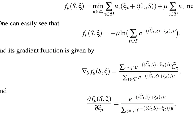
fµ(S) =min
u∈△τ∈
∑
DuτhXeτ,Si+µτ∈∑
Duτln uτ.We use the smoothed problem maxS∈P fµ(S)to approximate problem (19). It is easy to see that
fµ(S) =−µ ln
∑
τ∈DInput:
·smoothing parameter µ>0 (e.g., 10−5) ·tolerance value tol (e.g., 10−5)
·step sizes{αt ∈(0,1): t∈N} Initialization: Sµ1∈Sd
+ with Tr(S µ 1) =1 for t=1,2,3, . . .do
·Ztµ=arg max
fµ(St) +hZ,∇fµ(Sµt)i: Z∈Sd+,Tr(Z) =1 , that is, Ztµ=vv⊤
where v is the maximal eigenvector of matrix∇fµ(Sµt)
·Stµ+1= (1−αt)Sµt +αtZtµ
·if|fµ(Sµt+1)−fµ(Sµt)|<tol then break Output: d×d matrix Stµ∈Sd+
Table 1: Approximate Frank-Wolfe Algorithm for DML-eig
and
∇fµ(S) =∑τ∈
De−hXeτ,Si/µXeτ
∑τ∈De−hXeτ,Si/µ
.
Since fµis a smooth function, we can prove that its gradient is Lipschitz continuous.
Lemma 4. For any S1,S2∈
P
, thenk∇fµ(S1)−∇fµ(S2)k ≤CµkS1−S2k,
where Cµ=2 maxτ∈DkXeτk2/µ.
Proof. It suffices to seek∇2f
µ(S)k ≤2 maxτ∈DkXeτk2/µ.To this end,
∇2f
µ(S) = (∑τ∈De
−hXeτ,Si/µXe
τ)N(∑τ∈De−hXeτ,Si/µXeτ)
µ ∑τ∈De−hXeτ,Si/µ
2 −∑τ∈
De−hXeτ,Si/µXeτNXeτ
µ∑τ∈De−hXeτ,Si/µ
:=I+II,
where XNS denotes the tensor product of matrices X and S. We can estimate the term I as follows:
kIk ≤ ∑τ∈De
−hXeτ,Si/µkXe
τk ∑τ∈De−hXeτ,Si/µkXeτk
µ ∑τ∈De−hXeτ,Si/µ
2 ≤
1 µmaxτ∈D k
e
Xτk2,
where, in the above inequality, we used the fact thatkSNXk ≤ kXkkSk for any X,S∈Sd. The second term II can be similarly estimated:
kIIk ≤max τ∈D kXeτk
2/µ. Putting them together yields the desired result.
The pseudo-code to solve DML-eig is described in Table 1 which is a generalization of Frank-wolfe algorithm (Frank and Wolfe, 1956) which originally applies to the context of minimizing a convex function over a feasible polytope. Hazan (2008) first extended the original Frank-Wolfe algorithm to solve SDP over the spectrahedron
P
={M : M∈SdLemma 5. For any 0<µ≤1, let{Stµ: t ∈N}be generated by the algorithm in Table 1 and Cµ be defined in Lemma 4. Then we have that
max
S∈P fµ(S)−fµ(S
µ
t+1)≤Cµα2t + (1−αt) max
S∈P fµ(S)−f(S
µ t)
.
Proof. By the definition of Cµin Lemma 4, we have
fµ(Sµt+1)≥ fµ(Sµt) +αth∇fµ(Sµt),Zt−Sµti −Cµα2t. (20) Since f is concave, for any S∈
P
there holdsh∇fµ(Stµ),Zt−Stµi ≥ h∇fµ(Sµt),S−Stµi ≥fµ(S)−f(Sµt),
which implies that
h∇fµ(Sµt),Zt−Stµi ≥max
S∈P fµ(S)−fµ(S
µ t).
Substituting the above inequality into (20) yields the desired result.
For simplicity, let Rt =maxS∈P fµ(S)−fµ(Stµ). If αt ∈(0,1]for any t≥t0 with some t0∈N, then by Lemma 5 and a simple induction, for any t≥t0there holds
Rt+1≤Cµ t
∑
j=t0t
∏
k=j+1(1−αk)α2j+ t
∏
j=t0(1−αj)Rt0. (21)
Combining this inequality and some ideas in Ying and Zhou (2006), one can establish sufficient conditions on the stepsizes{αt : t∈N}such that limt→∞fµ(Stµ) =minS∈P fµ(S).
Theorem 6. For any fixed µ>0, let{Stµ: t∈N}be generated by the algorithm in Table 1. If the step sizes satisfy that
∑
t∈Nαt=∞, lim
t→∞αt =0, (22)
then
lim t→∞fµ(S
µ
t) =max S∈P fµ(S).
The detailed proof of the above theorem is given in Appendix B. Typical examples of step sizes satisfying condition (22) are{αt =t−θ: t∈N}with 0<θ≤1. For the particular caseθ=1, by Lemma 5 we can prove the following result.
Theorem 7. For any 0<µ≤1, let{Sµt : t∈N}be generated by Table 1 with step sizes given by
{αt =2/(t+1): t ∈N}.Then, for any t∈Nwe have that
max
S∈P fµ(S)−fµ(S
µ t)≤
8 maxτ∈DkXeτk2
µt +
4 ln D
t . (23)
Furthermore,
max
S∈P f(S)−f(S
µ
t)≤2µ ln D+
8 maxτ∈DkXeτk2
µt +
Proof. It is easy to see, for any S∈
P
that|f(S)−fµ(S)| ≤µ max
u∈△τ∈
∑
D(−uτln uτ)≤µ ln D.Let S∗=arg maxS∈P f(S)and Sµ∗=arg maxS∈P fµ(S). Then, for any t∈N,
maxS∈P f(S)−f(Sµt) = [f(S∗)−fµ(S∗)] + [fµ(S∗)−maxS∈P fµ(S)]
+[fµ(Sµ∗)−fµ(Sµt)] + [fµ(Sµt)−f(S µ t)]
≤[f(S∗)−fµ(S∗)] + [fµ(Sµ∗)−fµ(Sµt)] + [fµ(Sµt)−f(S µ t)]
≤2µ ln D+ [fµ(Sµ∗)−fµ(Stµ)]
=2µ ln D+ [maxS∈P fµ(S)−fµ(Stµ)].
Hence, it suffices to prove (23) by induction. Indeed, for t=1, we have that
maxS∈P fµ(S)−fµ(Sµ1) ≤ fµ(S∗µ) +µ supu∈△(∑τ∈D(−uτln uτ))
≤maxS∈Pminu∈△∑τ∈DuτhXeτ,Si+µ ln D
≤maxS∈Pminu∈△∑τ∈DuτkXeτkkSk+µ ln D
≤minu∈△∑τ∈DuτkXeτk+µ ln D
≤minu∈△
∑τ∈Duτ+∑τ∈DuτkXeτk2
+µ ln D ≤1+maxτ∈DkXeτk2+µ ln D,
which obviously satisfies (23) with t =1. Suppose the inequality (23) holds true for some t>1. Now by Lemma 5,
Rt+1 ≤Cµαt2+ (1−αt)Rt
≤ 4Cµ
(t+1)2+tt+−11
4Cµ
t + 4 ln D
t
≤4(Cµ+ln D) (t+11)2+(tt+−11)t
≤4(Cµ+ln D)
t+1 ,
where the second inequality follows from the induction assumption. This proves the inequality (23) for all t∈Nwhich completes the proof of the theorem.
By the above theorem, for any ε > 0, then µ = 4 ln Dε and the iteration number t ≥ 64(1+maxτ∈DkXeτk2)ln D/ε2 yields that maxS∈P f(S)−f(Sµt)≤ε. The time complexity of the approximate first-order method for DML-eig is of
O
d2/ε2.3.2 Approximate Frank-Wolfe Algorithm for LMNN-eig
We can easily extend the above approximate Frank-Wolfe algorithm to solve the eigenvalue opti-mization formulation of LMNN-eig (formulation (16) or (17)). To this end, let
f(S,ξ) =min
u∈△τ∈
∑
Duτ ξτ+hCeτ,Si.
Then, problem (16) is identical to
maxf(S,ξ):(1−γ)
∑
τ ξτ+γTr(S) =1,S∈
Sd
Input:
·smoothing parameter µ>0 (e.g., 10−5) ·tolerance value tol (e.g., 10−5)
·step sizes{αt∈(0,1): t∈N} Initialization: Sµ1∈Sd
+with Tr(S µ
1) =1 andξ µ 1≥0 for t=1,2,3, . . .do
·(Ztµ,βµt) =arg max
hZ,∂Sfµ(Stµ,ξµt)i+ξ⊤∂ξfµ(Sµt,ξµt): Z∈Sd+, ξ≥0
(1−γ)ξ⊤1+γTr(Z) =1 ·(St+µ 1,ξµt+1) = (1−αt)(Stµ,ξ
µ
t) +αt(Ztµ,β µ t)
·if|fµ(Sµt+1,ξt+µ 1)−fµ(Stµ,ξ µ
t)|<tol then break Output: d×d matrix Sµt ∈Sd+and slack variablesξµt
Table 2: Approximate Frank-Wolfe Algorithm for LMNN-eig
In analogy to the smooth techniques applied to DML-eig, we approximate f(S,ξ)by the following smooth function:
fµ(S,ξ) =min
u∈△τ∈
∑
Duτ(ξτ+hCeτ,Si) +µτ∈∑
Duτln uτ.One can easily see that
fµ(S,ξ) =−µ ln
∑
τ∈Te−(hCeτ,Si+ξτ)/µ.
and its gradient function is given by
∇Sfµ(S,ξ) =∑τ∈
Te−(hCeτ,Si+ξτ)/µCeτ
∑τ∈Te−(hCeτ,Si+ξτ)/µ
,
and
∂fµ(S,ξ) ∂ξτ =
e−(hCeτ,Si+ξτ)/µ ∑τ∈T e−(hCeτ,Si+ξτ)/µ
.
The approximate Frank-Wolfe algorithm for LMNN-eig is exactly the same as DML-eig in Table 1. The pseudo-code is listed in Table 2. The key step of the algorithm is to compute the following problem:
(Ztµ,βµt) =arg maxhZ,∂Sfµ(Stµ,ξ µ
t)i+ξ⊤∂ξfµ(Sµt,ξ µ
t): Z∈Sd+,ξ≥0
(1−γ)ξ⊤1+γTr(Z) =1 .
Equivalently, one needs to solve, for any A∈Sd andβ∈RT, the following problem:
(Z∗,ξ∗) =arg maxhZ,Ai+ξ⊤β: Z∈Sd
+,ξ≥0,(1−γ)ξ⊤1+γTr(Z) =1 . (24)
Letβmax=βτ∗ with τ∗∈
T
and v∗ is the largest eigenvector of A. Then, problem (24) is a linear programming and its optimal value is eithermaxξ⊤β:(1−γ)ξ⊤1=1,ξ≥0 =βmax
or
maxhZ,Ai:γTr(Z) =1,Z∈Sd
+ =
λmax(A)
γ .
The optimal solution of problem (24) is given as follows. If λmaxγ (A)>=βmax1−γ , then Z∗=v∗(vγ∗)⊤
where v∗is the largest eigenvector of matrix A andξ∗=0. Otherwise, Z∗=0 and theτ∗-th element of ξ∗ equals 1−γ1 , that is, (ξ∗)τ∗ = 1−γ1 and the other entries of ξ∗ all zeros. In analogy to the arguments for Theorem 7, for step sizes{αt=t+21: t∈N}one can exactly prove the time complexity of LMNN-eig is
O
(d2/ε2).4. Related Work and Discussion
There is a large amount of work on metric learning including distance metric learning for k-means clustering (Xing et al., 2002), relevant component analysis (RCA) (Bar-Hillel et al., 2005), max-imally collapsing metric learning (MCML) (Goldberger et al., 2004), neighborhood component analysis (NCA) (Goldberger et al., 2004) and an information-theoretic approach to metric learning (ITML) (Davis et al., 2007) etc. We refer the readers to Yang and Jin (2007) for a nice survey on metric learning. Below we discuss some specific metric learning models which are closely related to our work.
Xing et al. (2002) developed the metric learning model (2) to learn a Mahalanobis metric for k-means clustering. The main idea is to maximize the distance between points in the dissimilarity set under the constraint that the distance between points in the similarity set is upper-bounded. A projection gradient method is employed to obtain the optimal solution. Specifically, at each iteration the algorithm takes a gradient ascent step of the objective function and then projects it back to the set of constraints and the cone of the p.s.d. matrices. The projection to the p.s.d. cone needs the computation of the full eigen-decomposition with time complexity
O
(d3). The projection gradient method usually takes a large number of iterations to become convergent. It is worth mentioning that the metric learning model proposed in Xing et al. (2002) is a global method in the sense that the model aggregates all similarity constraints together as well as all dissimilarity constraints. In con-trast to Xing et al. (2002), DML-eig aims to maximize the minimal distance between dissimilar pairs instead of maximizing the summation of their distances. Consequently, DML-eig would intuitively force the dissimilar samples to be far more separated from similar samples. This intuition may account for the superior performance of DML-eig which will be shown soon in the experimental section.Weinberger et al. (2005) developed a large margin framework to learn a Mahalanobis distance metric for k-nearest neighbor (k-NN) classification (LMNN). The main intuition behind LMNN is that k-nearest neighbors always belong to the same class while examples from different classes are separated by a large margin. In contrast to the global method (Xing et al., 2002), LMNN is a local method in the sense that only triplets from the k-nearest neighbors are used. Our method DML-eig is a local method which only uses the similar pairs and dissimilar pairs from k-nearest neighbors.
Since every M ∈Sd
such dilemma will not happen. Specifically, Burer and Monteiro (2003) considered the following SDPs:
min
n
Tr(CM): Tr(AiM) =bi,i=1, . . . ,m,M∈Sd+
o
. (25)
It was proved that if A∗is a local minimum of the modified problem:
minnTr(CAA⊤): Tr(AiAA⊤) =bi,i=1, . . . ,m,A∈Rd×d
o ,
then M∗=A∗(A∗)⊤is a global minimum of the primal problem (25). However, since the hinge loss is not smooth, it is unclear how their proof can be adapted to the case of LMNN.
Rosales and Fung (2006) proposed the following element-sparse metric learning for high-dimensional data sets
min M∈Sd
+t=(i,
∑
j,k)∈T(1+x⊤i jMxi j−x⊤k jMxk j)++γ
∑
ℓ,k∈Nd|Mℓk|. (26)
In order to solve the optimization problem, they further proposed to restrict M to the space of diagonal dominance matrices which reduces formulation (26) to a linear programming problem. Such a restriction would only result in a sub-optimal solution.
Shalev-Shwartz et al. (2004) developed an appealing online learning model for learning a Ma-halanobis distance metric. In each time, given a pair of examples the p.s.d. distance matrix is updated by a rank-one matrix which only needs the time complexity
O
(d2).However, since the pairs of similarly labeled and differently labeled examples are usually of orderO
(n2), the online learning procedure takes many rank-one matrix updates. Jin et al. (2009) established generalization bounds for large margin metric learning and proposed an adaptive way to adjust the step sizes of the online metric learning method in order to guarantee the output matrix in each step is positive semi-definite. Since the pairs of similarity and dissimilarity are usually of orderO
(n2)where n is the sample number, the online learning procedure generally needs many matrix updates.Shen et al. (2009) recently employed the exponential loss for metric learning which can be written by
min M∈Sd
+τ=(i,
∑
j,k)∈TehCτ,Mi+Tr(M),
where
T
is the triplet set and Cτ= (xi−xj)(xi−xj)⊤−(xj−xk)(xj−xk)⊤for anyτ= (i,j,k)∈T
. A boosting-based algorithm called BoostMetric was developed which is based on the idea that each p.s.d. matrix can be decomposed into a linear positive combination of trace-one and rank-one matrices. The algorithm is essentially a column-generation scheme which iteratively finds the linear combination coefficients of the current basis set of rank-one matrices and then update the basis set of trace-one and rank-one matrices. The updating of rank-one and trace-one matrix only involves the computation of the largest eigenvector which is of time complexityO
(d2).However, the number of linear combination for the p.s.d. matrix can be infinite and the convergence rate of this column-generation algorithm is not clear.Data No. n d ♯class ♯
T
♯D
Wine 1 178 13 3 1134 378Iris 2 150 4 3 954 315
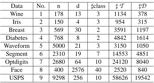
Breast 3 569 30 2 3591 1197 Diabetes 4 768 8 2 4842 1614 Waveform 5 5000 21 3 3150 1050 Segment 6 2310 19 7 14553 4851 Optdigits 7 2680 64 10 24120 8040 Face 8 400 2576 40 2520 840 USPS 9 9298 256 10 58626 19542
Table 3: Description of data sets n is the number of samples and d is the dimensionality. For AT&T face data set, we use PCA to reduce its dimension to 64.
5. Experiments
In this section we compare our proposed method DML-eig and LMNN-eig with a few methods: the method proposed in Xing et al. (2002) denoted by Xing, LMNN (Weinberger et al., 2005) and its accelerated version mLMNN (Weinberger and Saul, 2008), ITML (Davis et al., 2007), BoostMetric (Shen et al., 2009) and the baseline algorithm that uses the standard Euclidean distance denoted by Euc. For all the data sets we have set k=3 for nearest neighbor classification. The trade-off parameters in ITML, LMNN and LMNN-eig are tuned via three-fold cross validation. The smoothing parameter for DML-eig and LMNN-eig is set to be µ=10−4 and the maximum iteration for DML-eig, BoostMetric, LMNN-eig is set to be 103.
We first run experiments on 9 data sets, that is, 1) wine, 2) iris, 3) Breast-Cancer, 4) the Indian Pima Diabetes, 5) Waveform, 6) Segment, 7) Optdigits, 8) AT&T Face data set2and 9) USPS. The statistics of data sets summarized in Table 3. All experimental results are obtained by averaging over 10 runs (except 1 run for USPS due to its large size). For each run, we randomly split the data sets 70% for training and 30% for test validation. We have used the same mechanism in Weinberger et al. (2005) to generate training triplets. Briefly speaking, for each training point xi, k nearest neighbors that have same labels as yi (targets) as well as k nearest neighbors that have different labels from yi (imposers) are found. From xi and its corresponding targets and imposers, we then construct the set of similar pairs
S
(same labels) and the set of dissimilar pairsD
(distinct labels), and the set of tripletsT
. As mentioned above, the original formulation in Xing et al. (2002) used all pairwise constraints. We emphasize here, for fairness of comparison (especially the running time comparison), that all methods including the Xing’s method used the same set of similar/dissimilar pairs generated locally as above.Finally we will apply the developed models and algorithms on a large and challenging face verification data set called Labeled Faces in the Wild (LFW).3 It contains 13233 labeled faces of 5749 people, for 1680 people there are two or more faces. Furthermore, the data is challenging and difficult due to face variations in scale, pose, lighting, background, expression, hairstyle, and glasses, as the faces are detected in images in the wild, taken from Yahoo! News.
Euc. Xing LMNN ITML BoostMetric DML-eig LMNN-eig
1 3.46(3.60) 4.04(4.00) 3.08(2.07) 1.15(2.07) 2.31(2.18) 1.35(1.30) 2.88(1.87) 2 5.11(2.58) 6.67(3.11) 4.22(1.95) 4.44(2.57) 3.56(2.52) 3.11(1.15) 4.00(2.30)
3 6.47(1.33) 8.18 (1.58) 5.35(1.43) 6.82(1.57) 3.82(1.55) 3.53(0.88) 4.94(1.28)
4 31.09(2.03) 32.09 (3.56) 29.70(3.20) 29.96(2.97) 26.78(2.12) 27.71(3.93) 31.13(2.24) 5 18.87(0.65) 16.43(1.00) 18.61(0.72) 15.94(0.83) 16.86(0.90) 15.33(0.80) 18.49(0.21) 6 5.61(0.92) 5.26(0.60) 3.69(0.70) 5.02(0.70) 4.21(0.48) 2.97(0.55) 3.61(0.83) 7 1.67(0.24) 1.57(0.28) 1.37(0.25) 1.46(0.29) 1.38(0.33) 1.45(0.22) 1.43(0.42) 8 6.67(1.67) 7.75(0.69) 2.08(1.53) 2.42(2.17) 2.25(1.25) 1.67(1.24) 1.67(1.76)
9 3.05 - 2.98 3.92 3.34 3.66 3.13
Table 4: Average test error (%) of different metric learning methods (standard deviation are in parentheses). The best performance is denoted in bold type. The notation “–” means that the method does not converge in a reasonable time.
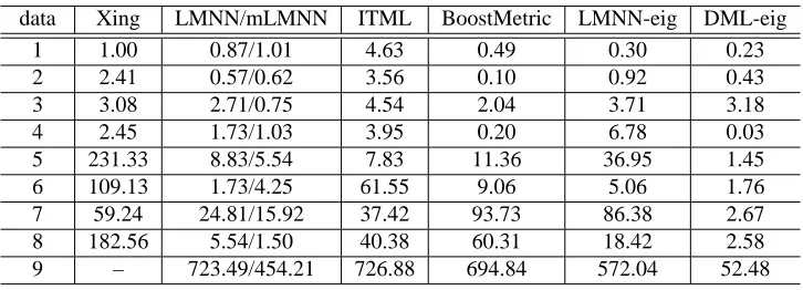
data Xing LMNN/mLMNN ITML BoostMetric LMNN-eig DML-eig
1 1.00 0.87/1.01 4.63 0.49 0.30 0.23
2 2.41 0.57/0.62 3.56 0.10 0.92 0.43
3 3.08 2.71/0.75 4.54 2.04 3.71 3.18
4 2.45 1.73/1.03 3.95 0.20 6.78 0.03
5 231.33 8.83/5.54 7.83 11.36 36.95 1.45
6 109.13 1.73/4.25 61.55 9.06 5.06 1.76
7 59.24 24.81/15.92 37.42 93.73 86.38 2.67
8 182.56 5.54/1.50 40.38 60.31 18.42 2.58
9 – 723.49/454.21 726.88 694.84 572.04 52.48
Table 5: Average running time (seconds) of different methods. The notation “–” means that the method does not converge in a reasonable time.
5.1 Generalization and Running Time
As we can see from Table 4, DML-eig consistently improves k-NN classification using Euclidean distance on most data sets. Hence, learning a Mahalanobis metric from training data does lead to improvements in k-NN classification. Also, we can see that DML-eig is competitive with the state-of-the-art methods: LMNN, ITML and BoostMetric. Indeed, DML-eig outperforms other algorithms on 5 out of 9 data sets. As expected, LMNN-eig performs similarly or slightly better than LMNN since these two models are essentially the same. In Table 5, we list the average CPU time of different algorithms. We can see that the method proposed in Xing et al. (2002) generally needs more time since it needs the full eigen-decomposition of a matrix per iteration. DML-eig, BoostMetric and LMNN are among the fastest algorithms while LMNN-eig is slower than LMNN and mLMNN in most cases. The accelerated version mLMNN is faster than LMNN.
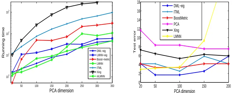
LMNN, BoostMetric, LMNN-eig and DML-eig are similar. As the dimension increases, DML-eig and mLMNN are faster. On this data set, LMNN-eig runs slower than mLMNN. The reason could be that mLMNN used the techniques of ball trees and employed only an active set of triplets per iteration. Our algorithms have not been combined with the techniques of ball trees and are imple-mented in MATLAB and better improvements are expected if used in C/C++. On the right-hand side of Figure 1, we also plot the test errors of various methods across different PCA dimensions. Al-most every method performs better than the baseline method using the standard Euclidean distance metric. DML-eig performs slightly better than other methods. We observe that, with increasing PCA dimensions, DML-eig, BoostMetric and ITML yield relatively stable performance across dif-ferent PCA dimensions. In contrast, the performance of other baseline methods such as LMNN and Xing’s method varied as the PCA dimensions changed.
50 100 150 200 250 300 350
100 101 102 103
PCA dimension
Running time
DML−eig LMNN−eig Boost−metric LMNN ITML Xing mLMNN
20 50 100 150 200 0
2 4 6 8 10 12 14 16 18
PCA dimension
Test error
DML−eig ITML BoostMetric PCA Xing LMNN
Figure 1: Performance on AT&T Face data set. Left figure: running time (seconds) versus PCA dimension. Right figure: test error (%) versus PCA dimension; the pink line is the per-formance of k-NN classifier (k=3) using the standard Euclidean distance.
5.2 Application to Face Verification
In this experiment we investigate our proposed method (DML-eig) for face verification. The task of face verification is to determine whether two face images are from the same identity or not. It is a highly active area of research and finds application in access control, image search, security and many other areas. The large variation in lighting, pose, expression etc. of the face images poses great challenges to the face verification algorithms. Inference that is based on the raw pixels of the image data or features extracted from the images is usually unreliable as the data show large variation and are high-dimensional.
The images we used are in gray scale and aligned in two ways. One is “funneled” (Huang et al., 2007) and the other is “aligned” using a commercial face alignment software by Taigman et al. (2009). These images are divided into ten folds where the subject identities are mutually exclusive. In each fold, there are 300 pairs of images from the same identity and another 300 pairs of images from different identities. We followed the standard procedure for training and test in the technical report of Huang et al. (2007). The performance of the algorithms is evaluated by average (and standard error of ) correct verification rate and the ROC curve of the 10-fold cross validation test.
We investigated several descriptors (features) from face images in this experiment. As for the “funneled” images, we used SIFT descriptors computed at the fixed facial key-points (e.g., corners of eyes and nose). These data are available from Guillaumin et al. (2009). We focus on the SIFT descriptor to evaluate our algorithm as it provides a fair comparison to Guillaumin et al. (2009). To compare with the state-of-the-art methods in face verification, we further investigated three types of features for the “aligned” images: 1) raw pixel data by concatenating the intensity value of each pixel in the image; 2) Local Binary Patterns (LBP) (Ojala et al., 2002); and 3) LBP’s variation, three-Patch Local Binary Patterns (TPLBP) (Wolf et al., 2008). The original dimensionality of the features is quite high (3456∼12000) so we reduced the dimension using PCA. These descriptors were tested with both their original value and the square root of them (Wolf et al., 2008, 2009; Guillaumin et al., 2009).
There are two configuration for forming the training sets. One is “restricted configuration”: only same/not-same labels are used during training and no information about the actual names of the people (class labels) in the image pairs should be used. In the past, most of the published work on this data set using the restricted protocol (e.g., Guillaumin et al., 2009; Wolf et al., 2009; Pinto et al., 2011). Another is “unrestricted configuration”: all available information including the names of the people in the images can be used for training. So far there are only two published results on the unrestricted configuration (Guillaumin et al., 2009; Taigman et al., 2009). Here we mainly focus on the restricted configuration.
LMNN and BoostMetric are not applicable in this restricted configuration setting since they need label information to generate the triplet set. Therefore, we only compared our DML-eig method with LDML (Guillaumin et al., 2009) and ITML (Davis et al., 2007). For each of the ten-fold cross-validation test, we use the data from 2700 pairs of images from the same identities and another 2700 pairs of images from the different identities to learn a metric. Then test it using the other 600 image pairs. The performance is evaluated using accurate verification rate .
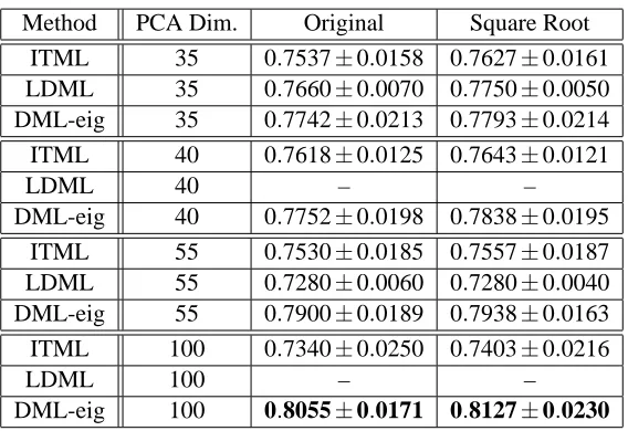
Table 6 illustrates the performances of our algorithm and ITML and LDML. The best verifica-tion rate of DML-eig is 81.27%. It outperforms LDML (77.50%) and ITML (76.20%) in their best settings. Note that the performance of DML-eig is consistently better than LDML and ITML in each PCA dimension.
Method PCA Dim. Original Square Root ITML 35 0.7537±0.0158 0.7627±0.0161 LDML 35 0.7660±0.0070 0.7750±0.0050 DML-eig 35 0.7742±0.0213 0.7793±0.0214 ITML 40 0.7618±0.0125 0.7643±0.0121
LDML 40 – –
DML-eig 40 0.7752±0.0198 0.7838±0.0195 ITML 55 0.7530±0.0185 0.7557±0.0187 LDML 55 0.7280±0.0060 0.7280±0.0040 DML-eig 55 0.7900±0.0189 0.7938±0.0163 ITML 100 0.7340±0.0250 0.7403±0.0216
LDML 100 – –
DML-eig 100 0.8055±0.0171 0.8127±0.0230
Table 6: Performance comparison on LFW database in the restricted configuration (mean verifica-tion accuracy and standard error of the mean of 10-fold cross validaverifica-tion test) with only SIFT descriptors. “Square Root” means the features preprocessed by taking square root before fed into metric learning method. The result of LDML is cited from Guillaumin et al. (2009) where it was reported that the best result of LDML is achieved with PCA dimension 35. Our result of ITML is very similar to that reported in Guillaumin et al. (2009).
Method Accuracy
High-Throughput Brain-Inspired Features, aligned (Pinto et al., 2011) 0.8813±0.0058 LDML + Combined, funneled (Guillaumin et al., 2009) 0.7927±0.0060 DML-eig + Combining four descriptors (this work) 0.8565±0.0056
Table 7: Performance comparison of DML-eig and other state-of-the-art methods in the restricted configuration (mean verification rate and standard error of the mean of 10-fold cross val-idation test) based on combination of different types of descriptors. The descriptors vary in different study. The best result up to date is achieved using sophisticated large scale feature search (Pinto et al., 2011).
20
40
60
80
100
120
140
160
0.7
0.72
0.74
0.76
0.78
0.8
0.82
Dimension of principal components
Verification rate
DML−eig
ITML
LDML
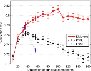
Figure 2: Performance of DML-eig, ITML and LDML metric by varying the dimension of the prin-cipal components using SIFT descriptor. The result of LDML is copied from Guillaumin et al. (2009).
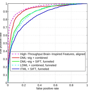
The best result reported to date is 88.13% in restricted configuration which performs sophis-ticated large scale feature search (Pinto et al., 2011). This work used multiple complimentary representations which are derived through training set augmentation, alternative face comparison functions, and feature set searches with a varying number of model layers. These individual feature representations are then combined using kernel techniques. The results by other state-of-the-art methods are also based on different descriptors (Guillaumin et al., 2009; Wolf et al., 2009). The best result achieved by DML-eig is 85.65%, which is close to the other state-of-the-art approaches. In addition, we note that the performance of DML-eig based on the single SIFT descriptor (81.27% in Table 6) is better than that of LDML based on 4 types of descriptors (79.27% in Table 7). The ROC curves of different methods are depicted in Figure 3. We can see that DML-eig outperforms ITML and LDML while it is suboptimal to the best up-to-date method (Pinto et al., 2011) which, however, employed sophisticated feature search method.
0 0.2 0.4 0.6 0.8 1 0
0.1 0.2 0.3 0.4 0.5 0.6 0.7 0.8 0.9 1
false positive rate
true positive rate High−Throughput Brain−Inspired Features, aligned
DML−eig + combined DML−eig + SIFT, funneled LDML + combined, funneled ITML + SIFT, funneled
Figure 3: ROC curve of DML-eig and other the state of arts methods for face verification on LFW data set.
6. Conclusion
The main theme of this paper is to develop a new eigenvalue-optimization framework for metric learning. Within this context, we first proposed a novel metric learning model which was shown to be equivalent to a well-known eigenvalue optimization problem (Overton, 1988; Lewis and Over-ton, 1996). This appealing optimization formulation was further extended to LMNN (Weinberger et al., 2005) and maximum margin matrix factorization (Srebro et al., 2004). Then, we developed efficient first-order algorithms for metric learning which only involve the computation of the largest eigenvector of a matrix. Their convergence rates were rigorously established. Finally, experiments on various data sets have shown that our proposed approach is competitive with state-of-the-art met-ric learning methods. In particular, we reported promising results on the Labeled Faces in the Wild (LFW) data set.
on the LFW data set in the unrestricted configuration setting, and embed the technique of ball trees (Weinberger and Saul, 2008) into our algorithms to further increase the computational speed.
Acknowledgments
The authors would like to thank Colin Campbell, Massimiliano Pontil, and Charles Micchelli for stimulating discussion and invaluable comments on the preliminary version of this paper. The au-thors also sincerely thank the anonymous reviewers for their comments and suggestions which have led to valuable improvements of this paper. This work is supported by the EPSRC under grant EP/J001384/1. The second author would like to thank Cancer Research UK for the research grant.
Appendix A. Eigenvalue Optimization for Maximum-margin Matrix Factorization
Another important problem is low-rank matrix completion which recently has attracted much atten-tion. This line of research involves computing a large matrix with a nuclear-norm (summation of singular values) regularization and the optimization problem here also consists of an SDP. Such tasks include multi-task feature learning (Argyriou et al., 2006) and low-rank matrix completion (Bach, 2008; Candes and Recht, 2008; Srebro et al., 2004). It has successful applications to collaborative filtering for predicting customers’ preferences to products, where the matrix’s rows and columns respectively identify the “customers” and “products”, and a matrix entry encodes customers’ pref-erence of a product (e.g., Netflix data set,http://www.netflixprize.com/).
Similar eigenvalue optimization formulation can be developed for maximum-margin matrix factorization (MMMF) for collaborative filtering (Srebro et al., 2004). Given a partially labeled Yia∈ {±1}with ia∈S, the target of MMMF is to learn a large matrix X∈Rm×nwhere each entry Xiaindicates the preference of the customer i for product a. The following large margin model was proposed in Srebro et al. (2004) to learn X :
minX ∑ia∈Sξia+γkXk∗ s.t. 1−YiaXia≤ξia,
ξia≥0,∀ia∈S,
wherekXk∗is the nuclear norm of X , that is, the summation of its singular values. The above model was further formulated as an SDP problem:
minM γTr(M) +∑ia∈Sξia
M= A X
X⊤ B
∈
S
+(m+n),YiaXia+ξia≥1,∀ia∈S.
(27)
Let eibe a column vector with its i-th element one and all others zero, then we have Mi(m+a)=Xia=
hCia,Miwith Cia=eie⊤(m+a).Consequently, the constraint condition in problem (27) can be written as minia∈ShYia,Ciai+ξia≥1. Using exact arguments for proving Theorem 3, we can formulate MMMF as an eigenvalue optimization problem.
Theorem 8. MMMF formulation (27) is equivalent to
maxnmin
u∈△ia
∑
∈Suia ξia+hYiaCia,Mi
In particular it is equivalent to the following eigenvalue optimization problem:
min u∈△max
umax,1
γλmax ia
∑
∈SuiaYiaCia
. (28)
As mentioned above, MMMF (27) is a standard SDP. Indeed, Srebro et al. (2004) proposed to employ standard SDP solvers (e.g., CSDP Borchers, 1999) to obtain the optimal solution. However, such generic solvers are only able to handle problems with about a hundred users and a hundred items. The eigenvalue-optimization formulation potentially provides more efficient algorithms for MMMF. Since the paper mainly focuses on metric learning, we leave its empirical implementation for future study.
Appendix B. Proof of Theorem 6
In this appendix we give the proof of Theorem 6. The spirit of the proof is very close to that of Theorem 1 in Ying and Zhou (2006) where similar conditions on step sizes were derived to guarantee the convergence of stochastic online learning algorithms in reproducing kernel Hilbert spaces.
Proof of Theorem 6. According to the assumption (22) on the step size, we can assume that, for any t≥t0, thatαt≤1/2. Hence, the inequality (21) holds true. We will estimate the terms on the left-hand side of (21) one by one.
For the second term on the righthand side of (21), observe that ∏tj=t0(1−αj) ≤ exp−∑tj=t0αj →0 as t→∞. Therefore, for anyε>0 there exists some t1∈N such that the second term on the righthand side of (21) is bounded byεwhenever t≥t1.
To deal with the first term on the righthand side of (21), we use the assumption limj→∞αj=0 and know that there exists some j(ε)such thatαj≤εfor every j≥ j(ε). Write
t
∑
j=t0 α2 j t∏
k=j+1(1−αk) = j(ε)
∑
j=t0 α2 j t∏
k=j+1(1−αk) + t
∑
j=j(ε)+1α2 j
t
∏
k=j+1(1−αk). (29)
Since j(ε)is fixed, we can find some t2∈Nsuch that for each t≥t2, there holds∑tj=t(ε)+1αj≥ ∑t2
j=j(ε)+1αj ≥log j(ε)
4ε . It follows that for each 1 ≤ j ≤ j(ε), there holds ∏ t
k=j+1(1−αk)≤ exp−∑tk=j+1αk ≤exp
−∑tk=j(ε)+1αk ≤ j(4εε). This in connection with the bound αj ≤1/2 for each j≥t0tells us that the first term of (29) is bounded as
t(ε)
∑
j=t0 α2 j t∏
k=j+1(1−αk)≤ 4ε j(ε)
j(ε)
∑
j=t0α2 j ≤ε.
The second term on the righthand side of (29) is dominated byε∑tj=−1j(ε)+1αj∏tk=j+1(1−αk). Noting the fact thatαj=1−(1−αj)implies
t
∑
j=j(ε)+1αj t
∏
k=j+1(1−αk) = t
∑
j=j(ε)+1h t
∏
k=j+1(1−αk)− t
∏
k=j(1−αk)
i
=h1−
t
∏
k=j(ε)+1(1−αk)
i