Distributed Submodular Maximization

(1)

Journal of Machine Learning Research 17 (2016) 1-44 Submitted 10/14; Published 12/16

Distributed Submodular Maximization

Baharan Mirzasoleiman [email protected]

Department of Computer Science ETH Zurich

Universitaetstrasse 6, 8092 Zurich, Switzerland

Amin Karbasi [email protected]

School of Engineering and Applied Science Yale University

New Haven, USA

Rik Sarkar [email protected]

Department of Informatics University of Edinburgh

10 Crichton St, Edinburgh EH8 9AB, United Kingdom

Andreas Krause [email protected]

Department of Computer Science ETH Zurich

Universitaetstrasse 6, 8092 Zurich, Switzerland

Editor:Jeff Bilmes

Abstract

Many large-scale machine learning problems–clustering, non-parametric learning, kernel machines, etc.–require selecting a small yet representative subset from a large dataset. Such problems can often be reduced to maximizing a submodular set function subject to various constraints. Classical approaches to submodular optimization require centralized access to the full dataset, which is impractical for truly large-scale problems. In this paper, we consider the problem of submodular function maximization in a distributed fashion. We develop a simple, two-stage protocolGreeDi, that is easily implemented using MapReduce style computations. We theoretically analyze our approach, and show that under certain natural conditions, performance close to the centralized approach can be achieved. We begin with monotone submodular maximization subject to a cardinality constraint, and then extend this approach to obtain approximation guarantees for (not necessarily mono-tone) submodular maximization subject to more general constraints including matroid or knapsack constraints. In our extensive experiments, we demonstrate the effectiveness of our approach on several applications, including sparse Gaussian process inference and exemplar based clustering on tens of millions of examples using Hadoop.

Keywords: distributed computing, submodular functions, approximation algorithms, greedy algorithms, map-reduce

1. Introduction

Numerous machine learning tasks require selecting representative subsets of manageable size out of large datasets. Examples range from exemplar based clustering (Dueck and

c

(2)

Mirzasoleiman, Karbasi, Sarkar and Krause

Frey, 2007) to active set selection for non-parametric learning (Rasmussen, 2004), to viral marketing (Kempe et al., 2003), and data subset selection for the purpose of training com-plex models (Lin and Bilmes, 2011). Many such problems can be reduced to the problem of

maximizing a submodular set functionsubject to cardinality or other feasibility constraints such as matroid, or knapsack constraints (Krause and Gomes, 2010; Krause and Golovin, 2012; Lee et al., 2009a).

Submodular functions exhibit a natural diminishing returns property common in many well known objectives: the marginal benefit of any given element decreases as we select more and more elements. Functions such as entropy or maximum weighted coverage are typical examples of functions with diminishing returns. As a result, submodular function optimization has numerous applications in machine learning and social networks: viral marketing (Kempe et al., 2003; Babaei et al., 2013; Mirzasoleiman et al., 2012), information gathering (Krause and Guestrin, 2011), document summarization (Lin and Bilmes, 2011), and active learning (Golovin and Krause, 2011; Guillory and Bilmes, 2011).

Although maximizing a submodular function is NP-hard in general, a seminal result of Nemhauser et al. (1978) states that a simple greedy algorithm produces solutions compet-itive with the optimal (intractable) solution (Nemhauser and Wolsey, 1978; Feige, 1998). However, such greedy algorithms or their accelerated variants (Minoux, 1978; Badanidiyuru and Vondr´ak, 2014; Mirzasoleiman et al., 2015a) do not scale well when the dataset is mas-sive. As data volumes in modern applications increase faster than the ability of individual computers to process them, we need to look at ways to adapt our computations using parallelism.

MapReduce (Dean and Ghemawat, 2008) is arguably one of the most successful pro-gramming models for reliable and efficient parallel computing. It works by distributing the data to independent machines: map tasks redistribute the data for appropriate parallel processing and the output then gets sorted and processed in parallel byreduce tasks.

To perform submodular optimization in MapReduce, we need to design suitable parallel algorithms. The greedy algorithms that work well for centralized submodular optimization do not translate easily to parallel environments. The algorithms are inherently sequential in nature, since the marginal gain from adding each element is dependent on the elements picked in previous iterations. This mismatch makes it inefficient to apply classical algorithms directly to parallel setups.

In this paper, we develop a distributed procedure for maximizing submodular functions, that can be easily implemented in MapReduce. Our strategy is to partition the data (e.g., randomly) and process it in parallel. In particular:

• We present a simple, parallel protocol, called GreeDi for distributed submodular maximization subject to cardinality constraints. It requires minimal communication, and can be easily implemented in MapReduce style parallel computation models.

• We show that under some natural conditions, for large datasets the quality of the obtained solution is provably competitive with the best centralized solution.

(3)

Distributed Submodular Maximization

• We implement our approach for exemplar based clustering and active set selection in Hadoop, and show how our approach allows to scale exemplar based clustering and sparse Gaussian process inference to datasets containing tens of millions of points.

• We extensively evaluate our algorithm on several machine learning problems, including exemplar based clustering, active set selection and finding cuts in graphs, and show that our approach leads to parallel solutions that are very competitive with those obtained via centralized methods (98% in exemplar based clustering, 97% in active set selection, 90% in finding cuts).

This paper is organized as follows. We begin in Section 2 by discussing background and related work. In Section 3, we formalize the distributed submodular maximization problem under cardinality constraints, and introduce example applications as well as naive approaches toward solving the problem. We subsequently present our GreeDi algorithm in Section 4, and prove its approximation guarantees. We then consider maximizing a submodular function subject to more general constraints in Section 5. We also present computational experiments on very large datasets in Section 6, showing that in addition to its provable approximation guarantees, our algorithm provides results close to the central-ized greedy algorithm. We conclude in Section 7.

2. Background and Related Work

2.1 Distributed Data Analysis and MapReduce

Due to the rapid increase in dataset sizes, and the relatively slow advances in sequen-tial processing capabilities of modern CPUs, parallel computing paradigms have received much interest. Inhabiting a sweet spot of resiliency, expressivity and programming ease, the MapReduce style computing model (Dean and Ghemawat, 2008) has emerged as prominent foundation for large scale machine learning and data mining algorithms (Chu et al., 2007; Ekanayake et al., 2008). A MapReduce job takes the input data as a set of < key;value > pairs. Each job consists of three stages: the map stage, the shuffle stage, and the reduce

stage. The map stage, partitions the data randomly across a number of machines by asso-ciating each element with a key and produce a set of < key;value > pairs. Then, in the shuffle stage, the value associated with all of the elements with the same key gets merged and send to the same machine. Each reducer then processes the values associated with the same key and outputs a set of new < key;value > pairs with the same key. The reduc-ers’ output could be an input to another MapReduce job, and a program in MapReduce paradigm can consist of multiple rounds of map and reduce stages (Karloff et al., 2010).

2.2 Centralized and Streaming Submodular Maximization

The problem of centralized maximization of submodular functions has received much inter-est, starting with the seminal work of Nemhauser et al. (1978). Recent work has focused on providing approximation guarantees for more complex constraints (for a more detailed account, see the recent survey by Krause and Golovin, 2012). Golovin et al. (2010) consider an algorithm for online distributed submodular maximization with an application to sensor selection. However, their approach requireskstages of communication, which is unrealistic

(4)

for large k in a MapReduce style model. Krause and Gomes (2010) consider the problem of submodular maximization in a streaming model; however, their approach makes strong assumptions about the way the data stream is generated and is not applicable to the general distributed setting. Recently, Badanidiyuru et al. (2014) provide a single pass streaming algorithm for cardinality-constrained submodular maximization with 1/2−εapproximation guarantee to the optimum solution that makes no assumptions on the data stream.

There has also been new improvements in the running time of the standard greedy solu-tion for solving SET-COVER (a special case of submodular maximizasolu-tion) when the data is large and disk resident (Cormode et al., 2010). More generally, Badanidiyuru and Vondr´ak (2014) and Mirzasoleiman et al. (2015a) improve the running time of the greedy algorithm for maximizing a monotone submodular function by reducing the number of oracle calls to the objective function. Very recently, Mirzasoleiman et al. (2016) provided a fast algorithm for maximizing non-monotone submodular functions under general constraints. In a similar spirit, Wei et al. (2014) propose a multi-stage framework for submodular maximization. In order to reduce the memory and computation cost, they apply an approximate greedy pro-cedure to maximize surrogate (proxy) submodular functions instead of optimizing the target function at each stage. The above approaches are sequential in nature and it is not clear how to parallelize them. However, they can be naturally integrated into our distributed framework to achieve further acceleration.

2.3 Scaling Up: Distributed Algorithms

(5)

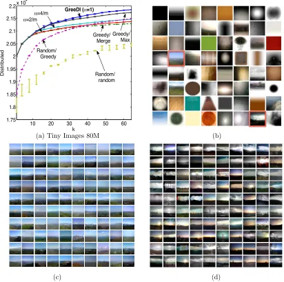
Figure 1: Cluster exemplars (left column) discovered by our distributed algorithm GreeDi described in Section 4 applied to the Tiny Images dataset (Torralba et al., 2008), and a set of representatives from each cluster.

3. Submodular Maximization

In this section, we first review submodular functions and how to greedily maximize them. We then describe thedistributed submodular maximization problem, the focus of this paper. Finally, we discuss two naive approaches towards solving this problem.

3.1 Greedy Submodular Maximization

Suppose that we have a large dataset of images, e.g., the set of all images on the Web or an online image hosting website such as Flickr, and we wish to retrieve a subset of images that best represents the visual appearance of the dataset. Collectively, these images can be considered as exemplars that summarize the visual categories of the dataset as shown in Fig. 1.

One way to approach this problem is to formalize it as the k-medoid problem. Given a set V = {e1, e2, . . . , en} of images (called ground set) associated with a (not necessarily symmetric) dissimilarity function, we seek to select a subsetS ⊆V of at mostkexemplars or cluster centers, and then assign each image in the dataset to its least dissimilar exemplar. If an element e ∈V is assigned to exemplar v ∈S, then the cost associated with e is the dissimilarity between e and v. The goal of the k-medoid problem is to choose exemplars that minimize the sum of dissimilarities between every data point e ∈V and its assigned cluster center.

Solving the k-medoid problem optimally is NP-hard, however, as we discuss in Section 3.4, we can transform this problem, and many other summarization tasks, to the problem of maximizing a monotone submodular function subject to a cardinality constraint

max

S⊆V f(S) s.t. |S| ≤k. (1)

Submodular functions are set functions which satisfy the following natural diminishing returns property.

Definition 1 (c.f., Nemhauser et al. (1978)) A set function f : 2V → _R is submodu-lar, if for every A⊆B ⊆V and e∈V \B

f(A∪ {e})−f(A)≥f(B∪ {e})−f(B).

Furthermore, f is called monotone iff for allA⊆B ⊆V it holds that f(A)≤f(B).

(6)

We will generally additionally require that f is nonnegative, i.e., f(A)≥0 for all sets A. Problem (1) is NP-hard for many classes of submodular functions (Feige, 1998). A fundamental result by Nemhauser et al. (1978) establishes that a simple greedy algorithm that starts with the empty set and iteratively augments the current solution with an element of maximum incremental value

v∗= arg max v∈V\Af(A

∪ {v}), (2)

continuing until k elements have been selected, is guaranteed to provide a constant factor approximation.

Theorem 2 (Nemhauser et al., 1978)For any non-negative and monotone submodular functionf, the greedy heuristic always produces a solution Agc[k] of size kthat achieves at least a constant factor (1−1/e) of the optimal solution.

f(Agc[k])≥(1−1/e) max

|A|≤kf(A).

This result can be easily extended to f(Agc[l])≥(1−e−l/k) max|A|≤kf(A), wherel and k are two positive integers (see, Krause and Golovin, 2012).

3.2 Distributed Submodular Maximization

In many today’s applications where the size of the ground set |V| = n is very large and cannot be stored on a single computer, running the standard greedy algorithm or its variants (e.g., lazy evaluations, Minoux, 1978; Leskovec et al., 2007; Mirzasoleiman et al., 2015a) in a centralized manner is infeasible. Hence, we seek a solution that is suitable for large-scale parallel computation. The greedy method described above is in general difficult to parallelize, since it is inherently sequential: at each step, only the object with the highest marginal gain is chosen and every subsequent step depends on the preceding ones.

Concretely, we consider the setting where the ground set V is very large and cannot be handled on a single machine, thus must be distributed among a set of m machines. While there are several approaches towards parallel computation, in this paper we consider the following model that can be naturally implemented in MapReduce. The computation proceeds in a sequence of rounds. In each round, the dataset is distributed to mmachines. Each machineicarries out computations independently in parallel on its local data. After all machines finish, they synchronize by exchanging a limited amount of data (of size polynomial in k and m, but independent of n). Hence, any distributed algorithm in this model must specify: 1) how to distribute V among them machines, 2) which algorithm should run on each machine, and 3) how to communicate and merge the resulting solutions.

(7)

3.3 Naive Approaches Towards Distributed Submodular Maximization

One way to solve problem (1) in a distributed fashion is as follows. The dataset is first partitioned (randomly, or using some other strategy) onto the m machines, with Vi rep-resenting the data allocated to machine i. We then proceed in k rounds. In each round, all machines–in parallel–compute the marginal gains of all elements in their sets Vi. Next, they communicate their candidate to a central processor, who identifies the globally best element, which is in turn communicated to themmachines. This element is then taken into account for computing the marginal gains and selecting the next elements. This algorithm (up to decisions on how break ties) implements exactly the centralized greedy algorithm, and hence provides the same approximation guarantees on the quality of the solution. Un-fortunately, this approach requires synchronization after each of the k rounds. In many applications, kis quite large (e.g., tens of thousands), rendering this approach impractical for MapReduce style computations.

An alternative approach for large k would be to greedily select k/m elements inde-pendently on each machine (without synchronization), and then merge them to obtain a solution of size k. This approach that requires only two rounds (as opposed tok), is much more communication efficient, and can be easily implemented using a single MapReduce stage. Unfortunately, many machines may select redundant elements, and thus the merged solution may suffer from diminishing returns. It is not hard to construct examples for which this approach produces solutions that are a factor Ω(m) worse than the centralized solution. In Section 4, we introduce an alternative protocol GreeDi, which requires little com-munication, while at the same time yielding a solution competitive with the centralized one, under certain natural additional assumptions.

3.4 Applications of Distributed Submodular Maximization

In this part, we discuss two concrete problem instances, with their corresponding submodu-lar objective functionsf, where the size of the datasets often requires a distributed solution for the underlying submodular maximization.

3.4.1 Large-scale Nonparametric Learning

Nonparametric learning (i.e., learning of models whose complexity may depend on the dataset size n) are notoriously hard to scale to large datasets. A concrete instance of this problem arises from training Gaussian processes or performing MAP inference in Deter-minantal Point Processes, as considered below. Similar challenges arise in many related learning methods, such as training kernel machines, when attempting to scale them to large data sets.

Active Set Selection in Sparse Gaussian Processes (GPs). Formally a GP is a joint probability distribution over a (possibly infinite) set of random variables XV, indexed by the ground set V, such that every (finite) subset XS for S = {e1, . . . , es} is distributed according to a multivariate normal distribution. More precisely, we have

P(XS =xS) =N(XS;µS,ΣS,S),

whereµ= (µe1, . . . , µes) and ΣS,S= [Kei,ej] are prior mean and covariance matrix,

respec-tively. The covariance matrix is parametrized via a positive definite kernel K(·,·). As a

(8)

concrete example, when elements of the ground setV are embedded in a Euclidean space, a commonly used kernel in practice is the squared exponential kernel defined as follows:

K(ei, ej) = exp(−||ei−ej||22/h2).

Gaussian processes are commonly used as priors for nonparametric regression. In GP regression, each data point e ∈ V is considered a random variable. Upon observations

yA=xA+nA(where nAis a vector of independent Gaussian noise with variance σ2), the predictive distribution of a new data point e ∈ V is a normal distribution P(Xe | yA) =

N(µe|A,Σ_e2|A), where meanµe|A and varianceσ

2

e|Aare given by

µe|A=µe+ Σe,A(ΣA,A+σ2I)−1(xA−µA), (3) σ_e2_|_A=σ_e2−Σe,A(ΣA,A+σ2I)−1ΣA,e. (4) Evaluating (3) and (4) is computationally expensive as it requires solving a linear system of |A| variables. Instead, most efficient approaches for making predictions in GPs rely on choosing a small–so calledactive–set of data points. For instance, in the Informative Vector Machine (IVM) one seeks a set S such that the information gain, defined as

f(S) =I(YS;XV) =H(XV)−H(XV|YS) = 1

2log det(I+σ

−2_Σ

S,S)

is maximized. It can be shown that this choice of f is monotone submodular (Krause and Guestrin, 2005a). For medium-scale problems, the standard greedy algorithms provide good solutions. For massive data however, we need to resort to distributed algorithms. In Section 6, we will show how GreeDi can choose near-optimal subsets out of a dataset of 45 million vectors.

Inference for Determinantal Point Processes. A very similar problem arises when per-forming inference in Determinantal Point Processes (DPPs). DPPs (Macchi, 1975) are distributions over subsets with a preference for diversity, i.e., there is a higher probability associated with sets containing dissimilar elements. Formally, a point processP on a set of items V ={1,2, ..., N} is a probability measure on 2V _{(the set of all subsets of} _V_). _P _is calleddeterminantal point process if for everyS⊆V we have:

P(S)∝det(KS),

where K is a positive semidefinite kernel matrix, and KS ≡[Kij]i,j∈S, is the restriction of K to the entries indexed by elements ofS (we adopt that det(K∅) = 1). The normalization

constant can be computed explicitly from the following equation

X S

det(KS) = det(I+K),

whereI is theN×N identity matrix. Intuitively, the kernel matrix determines which items are similar and therefore less likely to appear together.

(9)

3.4.2 Large-scale Exemplar Based Clustering

Suppose we wish to select a set of exemplars, that best represent a massive dataset. One approach for finding such exemplars is solving the k-medoid problem (Kaufman and Rousseeuw, 2009), which aims to minimize the sum of pairwise dissimilarities between ex-emplars and elements of the dataset. More precisely, let us assume that for the dataset V we are given a nonnegative function l : V ×V → R (not necessarily assumed symmetric, nor obeying the triangle inequality) such thatl(·,·) encodes dissimilarity between elements of the underlying set V. Then, the cost function for thek-medoid problem is:

L(S) = 1

|V|

X v∈V

min

e∈Sl(e, υ). (5)

Finding the subset

S∗ = arg min

|S|≤kL(S)

of cardinality at mostkthat minimizes the cost function (5) is NP-hard. However, by intro-ducing an auxiliary element e0, a.k.a. phantom exemplar, we can turn Linto a monotone

submodular function (Krause and Gomes, 2010)

f(S) =L({e0})−L(S∪ {e0}). (6)

In words, f measures the decrease in the loss associated with the set S versus the loss associated with just the auxiliary element. We begin with a phantom exemplar and try to find the active set that together with the phantom exemplar reduces the value of our loss function more than any other set. Technically, any pointe0 that satisfies the following

condition can be used as a phantom exemplar:

max v0_∈_V l(v, v

0

)≤l(v, e0), ∀v∈V \S.

This condition ensures that once the distance between any v ∈ V \S and e0 is greater

than the maximum distance between elements in the dataset, then L(S ∪ {e0}) = L(S).

As a result, maximizing f (a monotone submodular function) is equivalent to minimizing the cost function L. This problem becomes especially computationally challenging when we have a large dataset and we wish to extract a manageable-size set of exemplars, further motivating our distributed approach.

3.4.3 Other Examples

Numerous other real world problems in machine learning can be modeled as maximizing a monotone submodular function subject to appropriate constraints (e.g., cardinality, ma-troid, knapsack). To name a few, specific applications that have been considered range from efficient content discovery for web crawlers and multi topic blog-watch (Chierichetti et al., 2010), over document summarization (Lin and Bilmes, 2011) and speech data subset selection (Wei et al., 2013), to outbreak detection in social networks (Leskovec et al., 2007), online advertising and network routing (De Vries and Vohra, 2003), revenue maximization in social networks (Hartline et al., 2008), and inferring network of influence (Gomez Ro-driguez et al., 2010). In all such examples, the size of the dataset (e.g., number of webpages,

(10)

size of the corpus, number of blogs in the blogosphere, number of nodes in social networks) is massive, thus GreeDi offers a scalable approach, in contrast to the standard greedy algorithm, for such problems.

4. The GreeDi Approach for Distributed Submodular Maximization

In this section we present our main results. We first provide our distributed solution GreeDifor maximizing submodular functions under cardinality constraints. We then show how we can make use of the geometry of data inherent in many practical settings in order to obtain strong data-dependent bounds on the performance of our distributed algorithm.

4.1 An Intractable, yet Communication Efficient Approach

Before we introduceGreeDi, we first consider an intractable, but communication–efficient two-round parallel protocol to illustrate the ideas. This approach, shown in Algorithm 1, first distributes the ground set V to m machines. Each machine then finds the optimal

solution, i.e., a set of cardinality at mostk, that maximizes the value off in each partition. These solutions are then merged, and the optimal subset of cardinality k is found in the combined set. We denote this distributed solution byf(Ad[m, k]).

As the optimum centralized solution Ac[k] achieves the maximum value of the submod-ular function, it is clear that f(Ac[k]) ≥ f(Ad[m, k]). For the special case of selecting a single element k= 1, we havef(Ac[1]) =f(Ad[m,1]). Furthermore, for modularfunctions f (i.e., those for whichf and−f are both submodular), it is easy to see that the distributed scheme in fact returns the optimal centralized solution as well. In general, however, there can be a gap between the distributed and the centralized solution. Nonetheless, as the following theorem shows, this gap cannot be more than 1/min(m, k). Furthermore, this result is tight.

Theorem 3 Letf be a monotone submodular function and letk >0. Then,f(Ad[m, k]))≥ 1

min(m,k)f(A

c_[_k_])_{. In contrast, for any value of} _m _and _k_{, there is a monotone submodular}

functionf such that f(Ac[k]) = min(m, k)·f(Ad[m, k]).

The proof of all the theorems can be found in the appendix. The above theorem fully characterizes the performance of Algorithm 1 in terms of the best centralized solution. In practice, we cannot run Algorithm 1, since there is no efficient way to identify the optimum subsetAc_i[k] in set Vi, unless P=NP. In the following, we introduce an efficient distributed approximation – GreeDi. We will further show, that under some additional assumptions, much stronger guarantees can be obtained.

4.2 Our GreeDi Approximation

(11)

Algorithm 1 Inefficient Distributed Submodular Maximization

Input: SetV, #of partitions m, constraintsk.

Output: SetAd[m, k].

1: Partition V intom setsV1, V2, . . . , Vm.

2: In each partitionVi find the optimum setAci[k] of cardinality k. 3: Merge the resulting sets: B =∪m

i=1Aci[k].

4: Find the optimum set of cardinalityk inB. Output this solution Ad_[_{m, k}_].

Algorithm 2 Greedy Distributed Submodular Maximization (GreeDi)

Input: SetV, #of partitions m, constraintsκ.

Output: SetAgd[m, κ].

1: Partition V intom setsV1, V2, . . . , Vm (arbitrarily or at random).

2: Run the standard greedy algorithm on each setVi to find a solutionAgci [κ]. 3: Find Agcmax[κ] = arg maxA{F(A) :A∈ {Agc₁ [κ], . . . , Agcm[κ]}}

4: Merge the resulting sets: B =∪m i=1A

gc

i [κ].

5: Run the standard greedy algorithm on B to find a solution Agc_B[κ]. 6: Return Agd[m, κ] = arg maxA{F(A) :A∈ {Agcmax[κ], Agc_B[κ]}}.

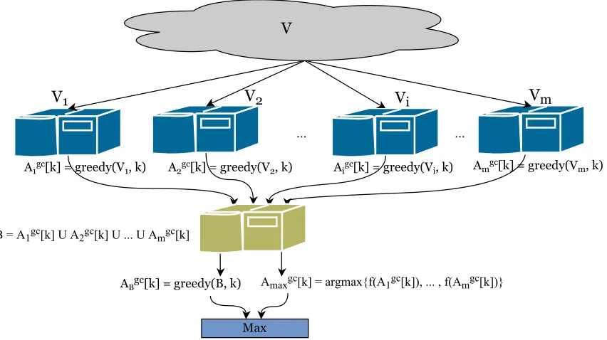
standard greedy algorithm by sequentially finding an element e ∈ Vi that maximizes the discrete derivative (2). Each machine i–in parallel–continues adding elements to the set Agc_i [·] until it reachesκ elements. We defineAgcmax[κ] to be the set with the maximum value

among {Agc₁ [κ], Agc₂ [κ], . . . , Agcm[κ]}. Then the solutions are merged, i.e., B = ∪mi=1A gc

i [κ], and another round of greedy selection is performed over B until κ elements are selected. We denote this solution by Agc_B[κ]. The final distributed solution with parameters m and κ, denoted by Agd[m, κ], is the set with a higher value between Agcmax[κ] and Agc_B[κ] (c.f.,

Figure 2 showsGreeDischematically). The following result parallels Theorem 3.

Theorem 4 Let f be a monotone submodular function and κ≥k. Then

f(Agd[m, κ])≥ (1−e −κ/k₎

min(m, k) f(A c_[_k_])_.

For the special case of κ =k the result of 4 simplifies to f(Agd[m, κ]) ≥ _min((1−1_m,k/e)₎f(Ac[k]). Moreover, it is straightforward to generalize GreeDi to multiple rounds (i.e., more than two) for very large datasets.

In light of Theorem 3, one can expect that in general it is impossible to eliminate the dependency of the distributed solution on min(k, m)1. However, as we show in the sequel, in many practical settings, the ground setV exhibits rich geometrical structure that can be used to obtain stronger guarantees.

1. It has been very recently shown by Mirzasoleiman et al. (2015b) that the tightest dependency is Θ(pmin(m, k)).

(12)

10/21/2014 Preview

1/1 ...

V

A1gc[k] = greedy(V1, k, FV1)

ABgc[k] = greedy(B, k, FU)

...

V_m V_i

V₁ V₂

A2gc[k] = greedy(V2, k, FV2) Aigc[k] = greedy(Vi, k, FVi) Amgc[k] = greedy(Vm, k, FVm)

B = A1gc[k] U A2gc[k] U ... U Amgc[k]

Amaxgc[k] = argmax{FU(A1gc[k]), ... , FU(Amgc[k])}

Max

... V

A1gc[k] = greedy(V1, k)

...

V_m V_i

V₁ V₂

A2gc[k] = greedy(V2, k) Aigc[k] = greedy(Vi, k) Amgc[k] = greedy(Vm, k)

ABgc[k] = greedy(B, k) Amaxgc[k] = argmax{f(A1gc[k]), ... , f(Amgc[k])}

Max

Figure 2: Illustration of our two-round algorithmGreeDi

4.3 Performance on Datasets with Geometric Structure

In practice, we can hope to do much better than the worst case bounds shown previously by exploiting underlying structure often present in real data and important set functions. In this part, we assume that a metricd:V ×V →_Rexists on the data elements, and analyze performance of the algorithm on functions that vary slowly with changes in the input. We refer to these as Lipschitz functions:

Definition 5 Let λ >0. A set function f : 2V →_R isλ-Lipschitz w.r.t. metricd onV, if for any integerk, any equal sized setsS ={e1, e2, . . . , ek} ⊆V andS0 ={e01, e02, . . . , e0k} ⊆V and any matching of elements: M = {(e1, e01),(e2, e02). . . ,(ek, e0k)}, the difference between f(S) and f(S0) is bounded by:

f(S)−f(S0) ≤λ

X i

d(ei, e0i). (7)

We can show that the objective functions from both examples in Section 3.4 areλ-Lipschitz for suitable kernels/distance functions:

Proposition 6 Suppose that the covariance matrix of a Gaussian process is parametrized via a positive definite kernel K : V ×V → R which is Lipschitz continuous with respect to metric d : V ×V → _R with constant L, i.e., for any triple of points x1, x2, x3 ∈ V, we have |K(x1, x3)− K(x2, x3)| ≤ Ld(x1, x2). Then, the mutual information I(YS;XV) =

1

(13)

Proposition 7 Letd:V×V →_Rbe a metric on the elements of the dataset. Furthermore, let l:V ×V →R encode the dissimilarity between elements of the underlying setV. Then for l = dα, α ≥ 1 the loss function L(S) = _|_V1_|P

v∈V mine∈Sl(e, υ) (and hence also the corresponding submodular utility functionf) isλ-Lipschitz with λ=αRα−1, whereR is the diameter of the ball encompassing elements of the dataset in the metric space. In particular, for the k-medoid problem, which minimizes the loss function over all clusters with respect to l =d, we have λ= 1, and for the k-means problem, which minimizes the loss function over all clusters with respect to l=d2, we have λ= 2R.

Beyond Lipschitz-continuity, many practical instances of submodular maximization can be expected to satisfy a natural density condition. Concretely, whenever we consider a representative set (i.e., optimal solution to the submodular maximization problem), we expect that any of its constituent elements has potential candidates for replacement in the ground set. For example, in our exemplar-based clustering application, we expect that cluster centers are not isolated points, but have many almost equally representative points close by. Formally, for any elementv∈V, we define itsα-neighborhoodas the set of elements inV within distanceα from v (i.e.,α-close tov):

Nα(v) ={w:d(v, w)≤α}.

By λ-Lipschitz-continuity, it must hold that if we replace element v in set S by an α -close element v0 (i.e., v0 ∈ Nα(v)) to get a new set S0 of equal size, it must hold that

|f(S)−f(S0)| ≤αλ.

As described earlier, our algorithm GreeDi partitions V into sets V1, V2, . . . Vm for parallel processing. If in addition we assume that elements are assigned uniformly at random to different machines, α-neighborhoods are sufficiently dense, and the submodular function is Lipschitz continuous, then GreeDi is guaranteed to produce a solution close to the centralized one. More formally, we have the following theorem.

Theorem 8 Under the conditions that 1) elements are assigned uniformly at random to m machines, 2) for eachei∈Ac[k]we have|Nα(ei)| ≥kmlog(k/δ1/m), and 3)f isλ-Lipschitz continuous, then with probability at least (1−δ) the following holds:

f(Agd[m, κ])≥(1−e−κ/k)(f(Ac[k])−λαk).

Note that once the above conditions are satisfied for small values of α (meaning that there is a high density of data points within a small distance from each element of the optimal solution) then the distributed solution will be close to the optimal centralized one. In particular if we letα→0, the distributed solution is guaranteed to be within a 1−eκ/k factor from the optimal centralized solution. This situation naturally corresponds to very large datasets. In the following, we discuss more thoroughly this important scenario.

4.4 Performance Guarantees for Very Large Datasets

Suppose that our dataset is a finite sample V drawn i.i.d. from an underlying infinite set

V, according to some (unknown) probability distribution. LetAc[k] be an optimal solution in the infinite set, i.e.,Ac[k] = arg maxS⊆Vf(S), such that around eachei∈Ac[k], there is

(14)

a neighborhood of radius at leastα∗ where the probability density is at leastβ at all points (for some constants α∗ and β). This implies that the solution consists of elements coming from reasonably dense and therefore representative regions of the dataset.

Let us suppose g : R → R is the growth function of the metric: g(α) is defined to be the volume of a ball of radius α centered at a point in the metric space. This means, for ei ∈ Ac[k] the probability of a random element being in Nα(ei) is at least βg(α) and the expected number of α neighbors of ei is at least E[|Nα(ei)|] = nβg(α). As a concrete example, Euclidean metrics of dimension D have g(α) =O(αD). Note that for simplicity we are assuming the metric to be homogeneous, so that the growth function is the same at every point. For heterogeneous spaces, we require g to have a uniform lower bound on the growth function at every point.

In these circumstances, the following theorem guarantees that if the dataset V is suffi-ciently large andf isλ-Lipschitz, thenGreeDiproduces a solution close to the centralized one.

Theorem 9 Forn ≥ 8kmlog(k/δ 1/m₎

βg(_λkε ) , where ε λk ≤α

∗_{, if the algorithm}

GreeDi assigns

elements uniformly randomly to m processors , then with probability at least(1−δ),

f(Agd[m, κ])≥(1−e−κ/k)(f(Ac[k])−ε).

The above theorem shows that for very large datasets, GreeDi provides a solution that is within a 1−eκ/k factor of the optimal centralized solution. This result is based on the fact that for sufficiently large datasets, there is a suitably dense neighborhood around each member of the optimal solution. Thus, if the elements of the dataset are partitioned uniformly randomly to m processors, at least one partition contains a set Ac_i[k] such that its elements are very close to the elements of the optimal centralized solution and provides a constant factor approximation of the optimal centralized solution.

4.5 Handling Decomposable Functions

So far, we have assumed that the objective function f is given to us as a black box, which we can evaluate for any given set S independently of the dataset V. In many settings, however, the objective f depends itself on the entire dataset. In such a setting, we cannot use GreeDi as presented above, since we cannot evaluate f on the individual machines without access to the full set V. Fortunately, many such functions have a simple structure which we call decomposable. More precisely, we call a submodular functionf decomposable

if it can be written as a sum of submodular functions as follows (Krause and Gomes, 2010):

f(S) = 1

|V|

X i∈V

fi(S)

(15)

10/21/2014 Preview

1/1 ...

V

A1gc[k] = greedy(V1, k, FV1)

ABgc[k] = greedy(B, k, FU)

...

V_m V_i

V₁ V₂

A2gc[k] = greedy(V2, k, FV2) Aigc[k] = greedy(Vi, k, FVi) Amgc[k] = greedy(Vm, k, FVm)

Amaxgc[k] = argmax{FU(A1gc[k]), ... , FU(Amgc[k])}

Max

...

V

A1gc[k] = greedy(V1, k)

...

V_m V_i

V₁ V₂

A2gc[k] = greedy(V2, k) Aigc[k] = greedy(Vi, k) Amgc[k] = greedy(Vm, k)

ABgc[k] = greedy(B, k) Amaxgc[k] = argmax{f(A1gc[k]), ... , f(Amgc[k])}

Max

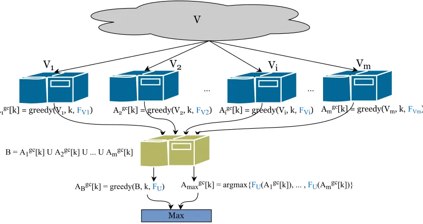
Figure 3: Illustration of our two-round algorithm GreeDifor decomposable functions

follows:

fD(S) = 1

|D|

X i∈D

fi(S)

In the remaining of this section, we show that assigning each element of the dataset randomly to a machine and runningGreeDiwill provide a solution that is with high probability close to the optimum solution. For this, let us assume that fi’s are bounded, and without loss of generality 0≤fi(S)≤1 for 1≤i≤ |V|, S ⊆V. Similar to Section 4.3 we assume that GreeDiperforms the partition by assigning elements uniformly at random to the machines. These machines then each greedily optimize fVi. The second stage of GreeDi optimizes

fU, whereU ⊆V is chosen uniformly at random with size dn/me.

Then, we can show the following result. First, for any fixed , m, k, let us define n0 to

be the smallest integer such that for n≥n0 we have ln(n)/n≤2/(mk).

Theorem 10 For n ≥ max(n0, mlog(δ/4m)/2), < 1/4, and under the assumptions of Theorem 9, we have, with probability at least 1−δ,

f(Agd[m, κ])≥(1−e−κ/k)(f(Ac[k])−2ε).

The above result demonstrates why GreeDi performs well on decomposable submodular functions with massive data even when they are evaluated locally on each machine. We will report our experimental results on exemplar-based clustering in the next section.

(16)

4.6 Performance of GreeDi on Random Partitions Without Geometric

Structure

Very recently, Barbosa et al. (2015) and Mirrokni and Zadimoghaddam (2015) proved that under random partitioning of the data amongmmachines, the expected utility of GreeDi will be only a constant factor away from the optimum.

Theorem 11 (Barbosa et al. (2015); Mirrokni and Zadimoghaddam (2015)) If el-ements are assigned uniformly at random to the machines, and κ = k, GreeDi gives a

constant factor approximation guarantee (in the average case) to the optimum centralized solution2.

E[f(Agd[m, k])]≥ 1

−1/e 2 f(A

c_[_k_])_.

These results show that random partitioning of the data is sufficient to guarantee that GreeDiprovides a constant factor approximation, irrespective ofmandk, and without the requirement of any geometric structure. On the other hand, if geometric structure is present, the bounds from the previous sections can provide sharper approximation guarantees.

5. (Non-Monotone) Submodular Functions with General Constraints

In this section we show howGreeDican be extended to handle 1) more general constraints, and 2) non-monotone submodular functions. More precisely, we consider the following optimization setting

Maximize f(S)

Subject to S∈ζ.

Here, we assume that the feasible solutions should be members of the constraint setζ ⊆2V_. The functionf(·) is submodular but may not be monotone. By overloading the notation we denote the set that achieves the above constrained optimization problem byAc[ζ]. Through-out this section we assume that the constraint set ζ is hereditary, meaning that if A ∈ ζ then for any B ⊆ A we also require that B ∈ ζ. Cardinality constraints are obviously hereditary, so are all the examples we mention below.

5.1 Matroid Constraints

A matroidMis a pair (V,I) whereV is a finite set (called the ground set) andI ⊆2V is a family of subsets ofV (called the independent sets) satisfying the following two properties:

• Heredity property: A⊆B ⊆V and B∈ I implies thatA∈ I, i.e. every subset of an independent set is independent.

• Augmentation property: IfA, B∈ I and|B|>|A|, there is an elemente∈B\A such thatA∪ {e} ∈ I.

(17)

Maximizing a submodular function subject to matroid constraints has found several applications in machine learning and data mining, ranging from content aggregation on the web (Abbassi et al., 2013) to viral marketing (Narayanam and Nanavati, 2012) and online advertising (Streeter et al., 2009).

One way to approximately maximize a monotone submodular functionf(S) subject to the constraint that each S is independent, i.e., S ∈ I, is to use a generalization of the greedy algorithm. This algorithm, which starts with an empty set and in each iteration picks the feasible element with maximum benefit until there is no more elementesuch that S∪ {e} ∈ I, is guaranteed to provide a 1₂-approximation of the optimal solution (Fisher et al., 1978). Recently, this bound has been improved to (1−1/e) using the continuous greedy algorithm (Calinescu et al., 2011). For non-negative and non-monotone submodular functions with matroid constraints, the best known result is a 0.325-approximation based on simulated annealing (Gharan and Vondr´ak, 2011).

Curvature: For a submodular functionf, the total curvature off with respect to a set S is defined as:

c= 1−min j∈V

f(j|S\j) f(j) .

Intuitively, the notion of curvature determines how far away f is from being modular. In other words, it measures how much the marginal gain of an element w.r.t. set S can decrease as a function of S. In general, c ∈ [0,1], and for additive (modular) functions, c = 0, i.e., the marginal values are independent of S. In this case, the greedy algorithm returns the optimal solution to max{f(S) :S ∈ I}. In general, the greedy algorithm gives a ₁₊1_c-approximation to maximizing a non-decreasing submodular function with curvature c subject to a matroid constraint (Conforti and Cornu´ejols, 1984). In case of the uniform matroid I ={S :|S| ≤k}, the approximation factor is (1−e−c)/c.

Intersection of Matroids: A more general case is when we have p matroids M₁ = (V,I1),M2 = (V,I2), ...,Mp= (V,Ip) on the same ground setV, and we want to maximize the submodular function f on the intersection of p matroids. That is, I =T

iIi consists of all subsets of V that are independent in all p matroids. This constraint arises, e.g., when optimizing over rankings (which can be modeled as intersections of two partition matroids). Another recent application considered is finding the influential set of users in viral marketing when multiple products need to be advertised and each user can tolerate only a small number of recommendations (Du et al., 2013). For p matroid constraints, the _p₊₁1 -approximation provided by the greedy algorithm (Fisher et al., 1978) has been improved to a (1_p−ε)-approximation forp≥2 by Lee et al. (2009b). For the non-monotone case, a 1/(p+ 2 + 1/p+ε)-approximation based on local search is also given by Lee et al. (2009b).

p-systems: p-independence systems generalize constraints given by the intersection of p matroids. Given an independence family I and a set V0 ⊆V, let S(V0) denote the set of maximal independent sets ofI included inV0, i.e.,S(V0) ={A∈ I | ∀e∈V0\A:A∪ {e}∈/

I}. Then we call (V,I) a p-system if for all nonempty V0 ⊆V we have

max

A∈S(V0₎|A| ≤p·_A_∈min_S₍_V0₎|A|.

(18)

Similar topmatroid constraints, the greedy algorithm provides a _p₊₁1 -approximation guar-antee for maximizing a monotone submodular function subject to a p-systems constraint (Fisher et al., 1978). For the non-monotone case, Gupta et al. (2010) provided a p/((p+ 1)(3p + 3))-approximation can be achieved by combining an algorithm of Gupta et al. (2010) with the result for unconstrained submodular maximization of Buchbinder et al. (2012). This result has been recently tightened to p/((p+ 1)(2p+ 1)) by Mirzasoleiman et al. (2016).

5.2 Knapsack Constraints

In many applications, including feature and variable selection in probabilistic models (Krause and Guestrin, 2005a) and document summarization (Lin and Bilmes, 2011), elementse∈V have non-uniform costsc(e)>0, and we wish to find a collection of elements S that maxi-mizef subject to the constraint that the total cost of elements inS does not exceed a given budget R, i.e.

max

S f(S) s.t. X v∈S

c(v)≤ R.

Since the simple greedy algorithm ignores cost while iteratively adding elements with max-imum marginal gains according (see Eq. 2) until |S| ≤ R, it can perform arbitrary poorly. However, it has been shown that taking the maximum over the solution returned by the greedy algorithm that works according to Eq. 2 and the solution returned by the modified greedy algorithm that optimizes the cost-benefit ratio

v∗ = arg max _e∈V\S c(v)≤R−c(S)

f(S∪ {e})−f(S) c(v) ,

provides a (1−1/√e)-approximation of the optimal solution (Krause and Guestrin, 2005b). Furthermore, a more computationally expensive algorithm which starts with all feasible so-lutions of cardinality 3 and augments them using the cost-benefit greedy algorithm to find the set with maximum value of the objective function provides a (1−1/e)-approximation (Sviridenko, 2004). For maximizing non-monotone submodular functions subject to knap-sack constraints, a (1/5−ε)-approximation algorithm based on local search was given by Lee et al. (2009a).

Multiple Knapsack Constraints: In some applications such as procurement auctions (Garg et al., 2001), video-on-demand systems and e-commerce (Kulik et al., 2009), we have ad-dimensional budget vectorRand a set of elemente∈V where each element is associated with ad-dimensional cost vector. In this setting, we seek a subset of elementsS ⊆V with a total cost of at most R that maximizes a non-decreasing submodular function f. Kulik et al. (2009) proposed a two-phase algorithm that provides a (1−1/e−ε)-approximation for the problem by first guessing a constant number of elements of highest value, and then taking the value residual problem with respect to the guessed subset. For the non-monotone case, Lee et al. (2009a) provided a (1/5−ε)-approximation based on local search.

(19)

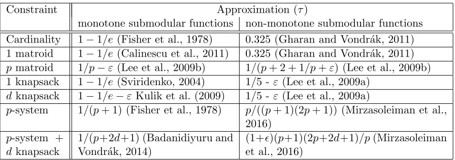
Constraint Approximation (τ)

monotone submodular functions non-monotone submodular functions Cardinality 1−1/e (Fisher et al., 1978) 0.325 (Gharan and Vondr´ak, 2011) 1 matroid 1−1/e (Calinescu et al., 2011) 0.325 (Gharan and Vondr´ak, 2011) p matroid 1/p−ε(Lee et al., 2009b) 1/(p+ 2 + 1/p+ε) (Lee et al., 2009b) 1 knapsack 1−1/e (Sviridenko, 2004) 1/5 - ε(Lee et al., 2009a)

dknapsack 1−1/e−εKulik et al. (2009) 1/5 - ε(Lee et al., 2009a)

p-system 1/(p+ 1) (Fisher et al., 1978) p/((p+ 1)(2p+ 1)) (Mirzasoleiman et al., 2016)

p-system + dknapsack

1/(p+2d+1) (Badanidiyuru and Vondr´ak, 2014)

(1+)(p+1)(2p+2d+1)/p(Mirzasoleiman et al., 2016)

Table 1: Approximation guarantees (τ) for monotone and non-monotone submodular max-imization under different constraints.

p-system with d knapsack constraints. For maximizing a monotone submodular function Badanidiyuru and Vondr´ak (2014) proposed a modified version of the greedy algorithm that guarantees a 1/(p+ 2d+ 1)-approximation. By combining this algorithm with the one proposed in (Gupta et al., 2010), Mirzasoleiman et al. (2016) provided a fast algorithm for maximizing a non-monotone submodular function subject to a p-system and d knapsack constraints with (1 +)(p+ 1)(2p+ 2d+ 1)/p-approximation.

Table 1 summarizes the approximation guarantees for monotone and non-monotone submodular maximization under different constraints.

5.3 GreeDi Approximation Guarantee under More General Constraints

Assume that we have a set of constraintsζ ⊆2V that is hereditary. Further assume we have access to a ”black box” algorithm X that gives us a constant factor approximation guar-antee for maximizing a non-negative (but not necessarily monotone) submodular function f subject to ζ, i.e.

X: (f, ζ)7→AX ∈ζ s.t. f(AX[ζ])≥τmax

A∈ζ f(A). (8)

We can modify GreeDi to use any such approximation algorithm as a black box, and provide theoretical guarantees about the solution. In order to process a large dataset, it first distributes the ground set overmmachines. Then instead of greedily selecting elements, each machine i–in parallel–separately runs the black box algorithm X on its local data in order to produce a feasible set AX_i [ζ] meeting the constraintsζ. We denote byAgcmax[ζ] the

set with maximum value among AX_i [ζ]. Next, the solutions are merged: B =∪m

i=1AXi [ζ], and the black box algorithm is applied one more time to setB to produce a solutionAgc_B[ζ]. Then, the distributed solution for parameter m and constraints ζ, AXd[m, ζ], is the best among Agcmax[ζ] and Agc_B[ζ]. This procedure is given in more detail in Algorithm 3.

The following result generalizes Theorem 4 for maximizing a submodular function sub-ject to more general constraints.

(20)

Algorithm 3 GreeDiunder General Constraints

Input: SetV, #of partitions m, constraintsζ, submodular functionf.

Output: SetAXd[m, ζ].

1: Partition V intom setsV1, V2, . . . , Vm.

2: In parallel: Run the approximation algorithm X on each setVito find a solutionAXi [ζ]. 3: Find Agcmax[ζ] = arg maxA{F(A)|A∈ {AX1 [ζ], . . . , AXm[ζ]}}.

4: Merge the resulting sets: B =∪m

i=1AXi [ζ].

5: Run the approximation algorithmX onB to find a solutionAgc_B[ζ]. 6: Return AXd[m, ζ] = arg max{Agcmax[ζ], Agc_B[ζ]}.

Theorem 12 Let f be a non-negative submodular function andX be a black box algorithm that provides aτ-approximation guarantee for submodular maximization subject to a set of hereditary constraints ζ. Then

f(AXd[m, ζ]))≥ τ

min m, ρ([ζ])f(A c_[_ζ_])_,

where f(Ac[ζ]) is the optimum centralized solution, and ρ([ζ]) = maxA∈ζ|A|.

Specifically, for submodular maximization subject to the matroid constraint M, we have ρ([A ∈ I]) = rM where rM is the rank of the matroid (i.e., the maximum size of any

independent set in the system). For submodular maximization subject to the knapsack constraint R, we can bound ρ([c(A) ≤ R]) by dR/minvc(v)e (i.e. the capacity of the knapsack divided by the smallest weight of any element).

Performance on Datasets with Geometric Structure. When the submodular func-tion f(·) and the constraint set ζ have more structure, then we can provide much better approximation guarantees. Assuming the elements ofV are embedded in metric space with distance d:V ×V → _R+_{, we say that} _ζ _is _{locally replaceable} _{with respect to a set} _S _⊆_V

with parameter α >0 if

∀S0 ⊆V s.t. |S0|=|S|and d∞(S, S0)≤α⇒S0 ∈ζ.

Here, we define the distance d∞ between two sets S and S0 of the same size k as follows.

LetM be the set of all possible matchings between S and S0, i.e.,

M ={((e1, e01), . . . ,(ek, e0k)) s.tei ∈S and e0i∈S0 for 1≤i≤k}.

Then d∞(S, S0) = minMmaxid(ei, e0i). We require locality only with respect to Ac[ζ] to ensure that the optimum solution can be well approximated. What the locally replaceable property requires is that as elements ofAc[ζ] get replaced by nearby elements, the resulting set is also a feasible solution. Combining this property withλ-Lipschitzness will provide us with the following theorem.

(21)

λ-Lipschitz, and 4)ζ is locally replaceable with respect toAc[ζ]with parameter α, then with probability at least (1−δ),

f(AXd[m, ζ]))≥τ(f(Ac[ζ])−λαρ([ζ])).

The above result generalizes Theorem 8 for maximizing non-negative submodular functions subject to different constraints.

Performance Guarantee for Very Large datasets. Similarly, we can generalize The-orem 9 for maximizing non-negative submodular functions subject to more general con-straints. Suppose that our dataset is a finite sample V drawn i.i.d. from an underlying

infinite set V, according to some (unknown) probability distribution. Let Ac[ζ] be an op-timal solution in the infinite set, i.e., Ac[ζ] = arg maxS⊆Vf(S), such that around each

ei∈Ac[ζ], there is a neighborhood of radius at least α∗ where the probability density is at least β at all points (for some constants α∗ and β). Recall that g :R → R is the growth function where g(α) measures the volume of a ball of radius α centered at a point in the metric space.

Theorem 14 Forn≥ 8ρ([ζ])mlog(ρ([ζ])/δ 1/m₎

βg(_λρ_([ε_ζ_])) , where ε λρ([ζ]) ≤α

∗_{, if}

GreeDiassigns

el-ements uniformly at random tomprocessors and under the conditions thatf isλ-Lipschitz, and ζ is locally replaceable with respect to Ac[ζ] with parameter α∗, then with probability at least (1−δ), we have

f(AXd[m, ζ]))≥τ(f(Ac[ζ])−ε).

Performance Guarantee for Decomposable Functions. For the case of decompos-able functions described in Section 4.5, the following generalization of Theorem 10 holds for maximizing a non-negative submodular function subject to more general constraints. Let us definen0 to be the smallest integer such that forn≥n0 we have ln(n)/n≤2/(m·ρ([ζ])). Theorem 15 For n ≥ max(n0, mlog(δ/4m)/2), < 1/4, and under the assumptions of Theorem 14, we have, with probability at least 1−δ,

f(AXd[m, ζ]))≥τ(f(Ac[ζ])−2ε).

6. Experiments

In our experimental evaluation we wish to address the following questions: 1) how well does GreeDiperform compared to the centralized solution, 2) how good is the performance of GreeDiwhen using decomposable objective functions (see Section 4.5), and finally 3) how well does GreeDi scale in the context of massive datasets. To this end, we run GreeDi on three scenarios: exemplar based clustering, active set selection in GPs and finding the maximum cuts in graphs.

We compare the performance of ourGreeDimethod to the following naive approaches:

• random/random: in the first round each machine simply outputs k randomly chosen elements from its local data points and in the second round k out of the merged mk elements, are again randomly chosen as the final output.

(22)

• random/greedy: each machine outputskrandomly chosen elements from its local data points, then the standard greedy algorithm is run overmkelements to find a solution of size k.

• greedy/merge: in the first roundk/melements are chosen greedily from each machine and in the second round they are merged to output a solution of sizek.

• greedy/max: in the first round each machine greedily finds a solution of sizek and in the second round the solution with the maximum value is reported.

ForGreeDi, we let each of themmachines select a set of sizeαk, and select a final solution of size k among the union of the m solutions (i.e., amongαkm elements). We present the performance of GreeDifor different parametersα >0. For datasets where we are able to find the centralized solution, we report the ratio of f(Adist[k])/f(Agc[k]), where Adist[k] is

the distributed solution (in particular Agd[m, αk, k] =Adist[k] forGreeDi).

6.1 Exemplar Based Clustering

Our exemplar based clustering experiment involvesGreeDiapplied to the clustering utility f(S) (see Sec. 3.4) with d(x, x0) = kx−x0k2_{. We performed our experiments on a set of}

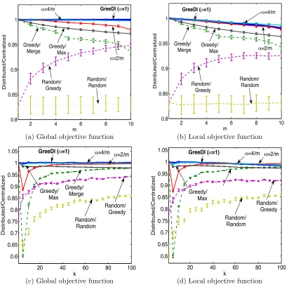
10,000 Tiny Images (Torralba et al., 2008). Each 32 by 32 RGB pixel image was repre-sented by a 3,072 dimensional vector. We subtracted from each vector the mean value, normalized it to unit norm, and used the origin as the auxiliary exemplar. Fig. 4a compares the performance of our approach to the benchmarks with the number of exemplars set to k = 50, and varying number of partitions m. It can be seen that GreeDi significantly outperforms the benchmarks and provides a solution that is very close to the centralized one. Interestingly, even for very small α=κ/k <1,GreeDiperforms very well. Since the exemplar based clustering utility function is decomposable, we repeated the experiment for the more realistic case where the function evaluation in each machine was restricted to the local elements of the dataset in that particular machine (rather than the entire dataset). Fig 4b shows similar qualitative behavior for decomposable objective functions.

Large scale experiments with Hadoop. As our first large scale experiment, we applied

(23)

2 4 6 8 10

0.8 0.85 0.9 0.95 1 m Distributed/Centralized Greedy/ Max Greedy/ Merge Random/ Random Random/ Greedy α=2/m

GreeDI (α=1)

α=4/m

(a) Global objective function

2 4 6 8 10

0.8 0.85 0.9 0.95 1 m Distributed/Centralized

GreeDI (α=1) _α_=4/m

Greedy/

Merge Greedy/Max α=2/m

Random/ Random Random/

Greedy

(b) Local objective function

20 40 60 80 100

0.6 0.65 0.7 0.75 0.8 0.85 0.9 0.95 1 1.05 k Distributed/Centralized

α=4/m _α_=2/m

Random/ Greedy Greedy/ Max GreeDI (α=1) Random/ Random Greedy/ Merge

(c) Global objective function

20 40 60 80 100

0.6 0.65 0.7 0.75 0.8 0.85 0.9 0.95 1 1.05 k Distributed/Centralized

α=4/m _α=2/m

Random/ Greedy Greedy/

Max GreeDI (α=1)

Random/ Random

(d) Local objective function

Figure 4: Performance of GreeDicompared to the other benchmarks. a) and b) show the mean and standard deviation of the ratio of distributed vs. centralized solution for global and local objective functions with budget k= 50 and varying the number m of partitions. c) and d) show the same ratio for global and local objective functions for m = 5 partitions and varying budget k, for a set of 10,000 Tiny Images.

6.2 Active Set Selection

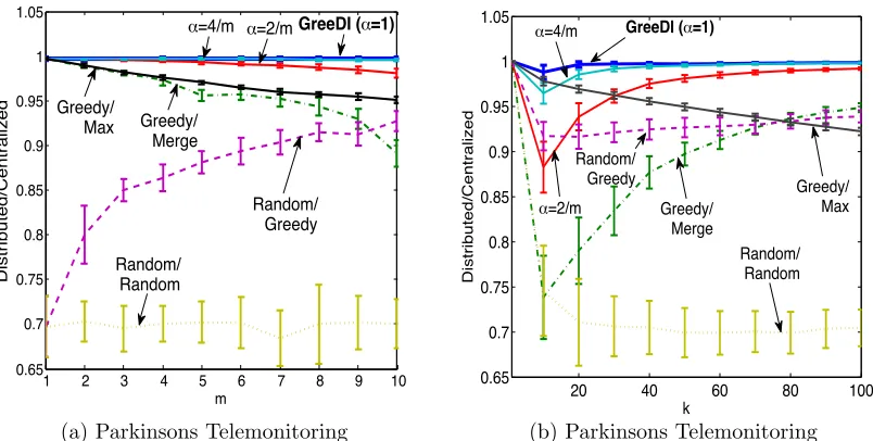
Our active set selection experiment involvesGreeDiapplied to the information gain f(S) (see Sec. 3.4) with Gaussian kernel,h= 0.75 andσ = 1. We used theParkinsons Telemon-itoring dataset (Tsanas et al., 2010) consisting of 5,875 bio-medical voice measurements with 22 attributes from people with early-stage Parkinson’s disease. We normalized the vectors to zero mean and unit norm. Fig. 6b compares the performance GreeDi to the

(24)

10 20 30 40 50 60

1.75 1.8 1.85 1.9 1.95 2 2.05 2.1 2.15

2.2x 10 4

k

Distributed

Random/ Greedy

α=4/m

α=2/m

Greedy/ Max Greedy/

Merge

Random/ random

GreeDI (α=1)

(a) Tiny Images 80M (b)

(c) (d)

Figure 5: Performance of GreeDi compared to the other benchmarks. a) shows the dis-tributed solution with m = 8000 and varying k for local objective functions on the whole dataset of 80,000,000 Tiny Images. b) shows a set of cluster exem-plars discovered byGreeDi, and each column in c) shows 100 images nearest to exemplars 26 and d) shows 100 images nearest to exemplars 63 in b).

benchmarks with fixedk= 50 and varying number of partitionsm. Similarly, Fig 6a shows the results for fixedm= 10 and varyingk. We find thatGreeDisignificantly outperforms the benchmarks.

Large scale experiments with Hadoop. Our second large scale experiment consists of

(25)

1 2 3 4 5 6 7 8 9 10

0.65 0.7 0.75 0.8 0.85 0.9 0.95 1 1.05

m

Distributed/Centralized

α=4/m α=2/mGreeDI (α=1)

Greedy/ Merge

Random/ Greedy

Random/ Random Greedy/

Max

(a) Parkinsons Telemonitoring

20 40 60 80 100

0.65 0.7 0.75 0.8 0.85 0.9 0.95 1 1.05

k

GreeDI (α=1) α=4/m

α=2/m Greedy/ Merge Random/

Greedy _Greedy/

Max

Random/ Random

(b) Parkinsons Telemonitoring

Figure 6: Performance of GreeDicompared to the other benchmarks. a) shows the ratio of distributed vs. centralized solution withk= 50 and varyingm forParkinsons Telemonitoring. b) shows the same ratio withm= 10 and varyingkon the same dataset.

of reducers set tom= 32. Each reducer performed the lazy greedy algorithm on its own set of≈1,431,621 vectors (≈34MB) in order to extract 256 elements with the highest marginal gains w.r.t the local elements of the dataset in that particular partition. We then merged the results and performed another round of lazy greedy selection on the merged results to extract the final active set of size 256. The maximum running time per reduce task was 12 minutes for selecting 128 elements and 48 minutes for selecting 256 elements. Fig. 7 shows the perfor-mance of GreeDicompared to the benchmarks. We note again thatGreeDisignificantly outperforms the other distributed benchmarks and can scale well to very large datasets.

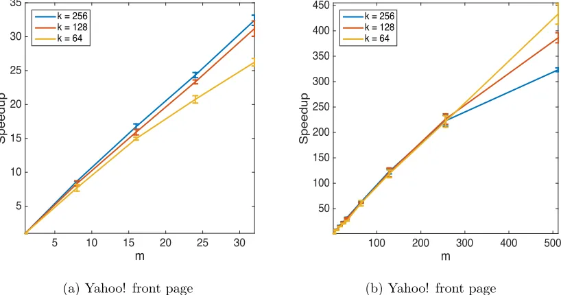
Performance Comparison. Fig. 8 shows the speedup of GreeDi compared to the

centralized greedy benchmark for different values of kand varying number of partitionsm. As Fig. 8a shows, for small values of m, the speedup is almost linear in the number of machines. However, for large values of m the running time of the second stage of GreeDi increases and ultimately dominates the whole running time. Hence, we do not observe a linear speedup anymore. This effect can be observed in Fig. 8b. For larger values ofk, the speedup is higher on fewer machines, but decreases more quickly by increasing m, as the second stage takes longer to complete.

6.3 Non-Monotone Submodular Function (Finding Maximum Cuts)

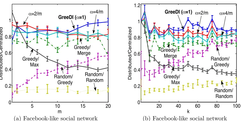
We also applied GreeDi to the problem of finding maximum cuts in graphs. In our set-ting we used a Facebook-like social network (Opsahl and Panzarasa, 2009). This dataset includes the users that have sent or received at least one message in an online student community at University of California, Irvine and consists of 1,899 users and 20,296 di-rected ties. Fig. 9a and 9b show the performance of GreeDi applied to the cut function on graphs. We evaluated the objective function locally on each partition. Thus, the links

(26)

k

0 50 100 150 200 250

0.5 0.6 0.7 0.8 0.9 1 1.1

GreeDI (,=1)

Greedy/ Max

,=4/m ,=2/m

Random/ Greedy

Merge

Figure 7: Performance of GreeDi with m = 32 and varying budget k compared to the other benchmarks onYahoo! Webscope data.

m

5 10 15 20 25 30

Speedup

5 10 15 20 25 30 35

k = 256 k = 128 k = 64

(a) Yahoo! front page

m

100 200 300 400 500

Speedup

50 100 150 200 250 300 350 400 450

k = 256 k = 128 k = 64

(b) Yahoo! front page

Figure 8: Running time of GreeDicompared to the centralized greedy algorithm. a) shows the ratio of centralized vs. distributed solution with k = 64,128,256 and up to m = 32 machines for Yahoo Webscope data. b) shows the same ratio with k = 64,128,256 and up tom= 512 machines on the same dataset. Both experiments are performed on a cluster of 8 quad core machines.

(27)

5 10 15 20

0 0.2 0.4 0.6 0.8 1

m

Distributed/Centralized Random/

Greedy

Max

Greedy/ Merge

α=2/m α=4/m

GreeDI (α=1)

(a) Facebook-like social network

20 40 60 80 100

0 0.2 0.4 0.6 0.8 1 1.2

k

Random/ Random

α=2/m α=4/m

GreeDI (α=1)

Random/ Greedy

Greedy/ Max Greedy/

Merge

(b) Facebook-like social network

Figure 9: Performance of GreeDicompared to the other benchmarks. a) shows the mean and standard deviation of the ratio of distributed to centralized solution for bud-getk= 20 with varying number of machines m and b) shows the same ratio for varying budgetk withm= 10 on Facebook-like social network.

Although the cut function does not decompose additively over individual data points, perhaps surprisingly, GreeDi still performs very well, and significantly outperforms the benchmarks. This suggests that our approach is quite robust, and may be more generally applicable.

6.4 Comparision with Greedy Scaling.

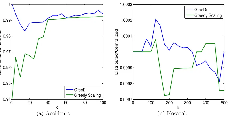
Kumar et al. (2013) recently proposed an alternative approach–GreedyScaling–for par-allel maximization of submodular functions. GreedyScalingis a randomized algorithm that carries out a number (typically less than k) rounds of MapReduce computations. We appliedGreeDito the submodular coverage problem in which given a collection V of sets, we would like to pick at most k sets fromV in order to maximize the size of their union. We compared the performance of our GreeDi algorithm to the reported performance of GreedyScalingon the same datasets, namelyAccidents (Geurts et al., 2003) andKosarak (Bodon, 2012). As Fig 10a and 10b shows, GreeDioutperformsGreedyScalingon the

Accidents dataset and its performance is comparable to that of GreedyScaling in the

Kosarakdataset.

7. Conclusion

We have developed an efficient distributed protocol GreeDi, for constrained submodular maximization. We have theoretically analyzed the performance of our method and showed that under certain natural conditions it performs very close to the centralized (albeit im-practical in massive datasets) solution. We have also demonstrated the effectiveness of our approach through extensive experiments, including active set selection in GPs on a dataset

(28)

0 20 40 60 80 100

0.94 0.95 0.96 0.97 0.98 0.99 1

k

GreeDi Greedy Scaling

(a) Accidents

0 100 200 300 400 500 0.9997

0.9998 0.9999 1 1.0001 1.0002 1.0003

k

GreeDi Greedy Scaling

(b) Kosarak

Figure 10: Performance of GreeDi compared to the GreedyScaling algorithm of Kumar et al. (2013) (as reported in their paper). a) shows the ratio of distributed to centralized solution on Accidents dataset with 340,183 elements and b) shows the same ratio for Kosarak dataset with 990,002 elements. The results are reported for varying budget kand varying number of machines m=n/µwhere µ= O(knδ_log_n_{) and} _n _{is the size of the dataset. The results are reported for} δ = 1/2. Note that the results presented by Kumar et al. (2013) indicate that GreedyScaling generally requires a substantially larger number of MapReduce rounds compared toGreeDi.

of 45 million examples, and exemplar based summarization of a collection of 80 million images using Hadoop. We believe our results provide an important step towards solving submodular optimization problems in very large scale, real applications.

Acknowledgments

This research was supported by SNF 200021-137971, DARPA MSEE FA8650-11-1-7156, ERC StG 307036, a Microsoft Faculty Fellowship, an ETH Fellowship, Google Research Faculty Award, and a Scottish Informatics and Computer Science Alliance.

Appendix A. Proofs

(29)

A.1 Proof of Theorem 3 ⇒ direction:

The proof easily follows from the following lemmas.

Lemma 16 max i f(A

c i[k])≥

1 mf(A

c_[_k_])_.

Proof Let Bi be the elements in Vi that are contained in the optimal solution, Bi = Ac[k]∩Vi. Then we have:

f(Ac[k]) =f(B1∪. . .∪Bm) =f(B1) +f(B2|B1) +. . .+f(Bm|Bm−1, . . . , B1).

Using submodularity off, for each i∈ {1. . . m}, we have

f(Bi|Bi−1. . . B1)≤f(Bi), and thus,

f(Ac[k])≤f(B1) +. . .+f(Bm). Since,f(Ac_i[k])≥f(Bi), we have

f(Ac[k])≤f(Ac₁[k]) +. . .+f(Ac_m[k]). Therefore,

f(Ac[k])≤m max i f(A

c

i[k]).

Lemma 17 max i f(A

c i[k])≥

1 kf(A

c_[_k_])_.

Proof Let f(Ac_[_k_{]) =}_f₍_{_u

1, . . . uk}). Using submodularity of f, we have f(Ac[k])≤

k X i=1

f(ui).

Thus,f(Ac[k])≤kf(u∗) whereu∗= arg max_if(ui). Suppose that the element with highest marginal gain (i.e., u∗) is in Vj. Then the maximum value of f on Vj would be greater or equal to the marginal gain of u∗, i.e., f(Ac_j[k]) ≥ f(u∗) and since f(maxif(Aci[k])) ≥ f(Ac_j[k]), we can conclude that

f(max i f(A

c

i[k]))≥f(u∗)≥ 1 kf(A

c_[_k_])_.

Since f(Ad[m, k])≥maxif(Aci[k]); from Lemma 16 and 17 we have f(Ad[m, k])≥ 1

min(m, k)f(A

c_[_k_])_.