Transfer Learning via Inter-Task Mappings
for Temporal Difference Learning
Matthew E. Taylor [email protected]
Peter Stone [email protected]
Yaxin Liu [email protected]
Department of Computer Sciences The University of Texas at Austin Austin, Texas 78712-1188
Editor: Michael L. Littman
Abstract
Temporal difference (TD) learning (Sutton and Barto, 1998) has become a popular reinforcement learning technique in recent years. TD methods, relying on function approximators to generalize learning to novel situations, have had some experimental successes and have been shown to exhibit some desirable properties in theory, but the most basic algorithms have often been found slow in practice. This empirical result has motivated the development of many methods that speed up re-inforcement learning by modifying a task for the learner or helping the learner better generalize to novel situations. This article focuses on generalizing across tasks, thereby speeding up learning, via a novel form of transfer using handcoded task relationships. We compare learning on a com-plex task with three function approximators, a cerebellar model arithmetic computer (CMAC), an artificial neural network (ANN), and a radial basis function (RBF), and empirically demonstrate that directly transferring the action-value function can lead to a dramatic speedup in learning with all three. Using transfer via inter-task mapping (TVITM), agents are able to learn one task and then markedly reduce the time it takes to learn a more complex task. Our algorithms are fully implemented and tested in the RoboCup soccer Keepaway domain.
This article contains and extends material published in two conference papers (Taylor and Stone, 2005; Taylor et al., 2005).
Keywords: transfer learning, reinforcement learning, temporal difference methods, value function approximation, inter-task mapping
1. Introduction
Machine learning has traditionally been limited to training and testing on the same distribution of problem instances. However, humans are able to learn to perform well in complex tasks by utilizing principles learned in previous tasks. Few current machine learning methods are able to transfer knowledge between pairs of tasks, and none are able to transfer between a broad range of tasks to the extent that humans are. This article presents a new method for transfer learning in the reinforcement learning (RL) framework using temporal difference (TD) learning methods (Sutton and Barto, 1998), whereby an agent can learn faster in a target task after training on a different, typically less complex, source task.
However, the basic unenhanced TD algorithms, such as Q-Learning (Watkins, 1989) and Sarsa (Rummery and Niranjan, 1994; Singh and Sutton, 1996), have been found slow to produce near-optimal behaviors in practice. Many techniques exist (Selfridge et al., 1985; Colombetti and Dorigo, 1993; Asada et al., 1994) which attempt, with more or less success, to speed up the learning process. Section 9 will discuss in depth how our transfer learning method differs from other existing methods and can potentially be combined with them if desired.
In this article we introduce transfer via inter-task mapping (TVITM), whereby a TD learner trained on one task with action-value function RL can learn faster when training on another task with related, but different, state and action spaces. TVITMthus enables faster TD learning in situations where there are two or more similar tasks. This transfer formulation is analogous to a human being told how a novel task is related to a known task, and then using this relation to decide how to perform the novel task. The key technical challenge is mapping an action-value function—the expected return or value of taking a particular action in a particular state—in one representation to a meaningful action-value function in another, typically larger, representation. It is this transfer functional which defines transfer in theTVITMframework.
In stochastic domains with continuous state spaces, agents will rarely (if ever) visit the same state twice. It is therefore necessary for learning agents to use function approximation when esti-mating the action-value function. Without some form of approximation, an agent would only be able to predict a value for states that it had previously visited. In this work we are primarily concerned with a different kind of generalization. Instead of finding similarities between different states, we focus on exploiting similarities between different tasks.
The primary contribution of this article is an existence proof that there are domains in which it is possible to construct a mapping between tasks and thereby speed up learning by transferring an action-value function. This approach may seem counterintuitive initially: the action-value function is the learned information which is directly tied to the particular task it was learned in. Neverthe-less, we will demonstrate the efficacy of usingTVITMto speed up learning in agents across tasks, irrespective of the representation used by the function approximator. Three different function ap-proximators (as defined in Section 4.3), a CMAC, an ANN, and an RBF, are used to learn a single reinforcement learning problem. We will compare their effectiveness and demonstrate whyTVITM
is promising for future transfer studies.
The remainder of this article is organized as follows. Section 2 formally defines TVITM.
Sec-tion 3 gives an overview of the tasks over which we quantitatively test our transfer method. SecSec-tion 4 gives details of learning in our primary domain, robot soccer Keepaway. Section 5 describes how we perform transfer in our selected tasks. Sections 6 and 7 present the results of our experiments. Section 8 discusses some of their implications and future work. Section 9 details other related work while contrasting our methods and Section 10 concludes.
2. Transfer via Inter-Task Mapping
TVITMis defined for value function reinforcement learners. Thus, to formally define how to use our transfer method we first briefly review the general reinforcement learning framework that conforms to the generally accepted notation for Markov decision processes (MDP) (Puterman, 1994).
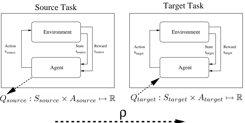
ρ
Environment
Agent
Environment
Agent
a s
Reward r
Action State
source source source
Source Task
Target Task
a s
Reward r
Action State
target target target
Figure 1: ρ is a functional that transforms a state-action function Q from one task so that it is applicable in a second task with different state and action spaces.
set of actions, A, which the agent can perform. The reward function, R : S7→R, maps each state of the environment to a single number which is the instantaneous reward achieved for reaching the state. The transition function, T : S×A7→S, takes a state and an action and returns the state of the environment after the action is performed. If transitions are non-deterministic the transition function is a probability distribution function. A learner is able to sense the current state, s, and typically knows A and what state variables comprise S. However, it does not know R, how it is rewarded for moving between states, or T , how actions move the agent between states.
A learner chooses which action to take in a given perceived environmental state by using a policy, π: S7→A. π is modified by the learner over time to improve performance, the expected total reward accumulated, and it completely defines the behavior of the learner in an environment. In the general case the policy can be stochastic. The success of an agent is determined by how well it maximizes the total reward it receives in the long run while acting under some policyπ. An
optimal policy,π∗, is a policy that maximizes the expectation of this value. Any reasonable learning
algorithm attempts to modifyπover time so that the agent’s performance approaches that ofπ∗in the limit. Value function reinforcement learning relies on learning a value function V : S7→Rso that the learner is able to estimate the total discounted reward that would be accumulated from moving to state s and then following the current policyπ. In practice, the action-value function Q : S×A7→R
is often learned, which frees the learner from having to explicitly model the transition function. If the action-value function is optimal (i.e., Q = Q∗),π∗ can be followed by always selecting the optimal action a, which is the action with the largest value of Q(s,a)in the current state.
action-value function may not provide immediate improvement over acting randomly in the target task, but it should bias the learner so that it is able to learn the target task faster than if it were learning without transfer.
A transfer functional ρ(Q) will allow us to apply a policy in a new task (see Figure 1). The policy transform functionalρneeds to modify the action-value function so that it accepts Starget as inputs and allows for Atarget to be outputs. A policy generally selects the action which is believed to accumulate the largest expected total reward; the problem of transforming a policy between two tasks therefore reduces to transforming the action-value function. Definingρto do this correctly is the key technical challenge to enable generalTVITM.
2.1 Constructing a Transfer Functional
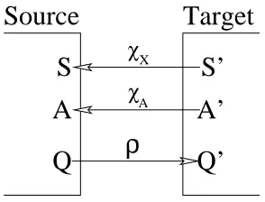
Given an arbitrary pair of unknown tasks and no experience in the pair of tasks, one could not hope to correctly defineρ, the transfer functional (for example, there are certainly pairs of tasks which have no relationship and thus mastery in one task would not lead to improved performance in the other). For our transfer method to succeed, not only must the two tasks be related, but we should be able to characterize how they are related. We represent these relations as a pair of inter-task mappings, denoted χX andχA. State variables in the target task are mapped via χX to the most
similar state variable in the source task:
χX(xi,target) =xj,source.
Similarly,χA maps each action in the target task to the most similar action in the source tasks:
χA(ai,target) =aj,source.
χX andχA, mappings from the target task to the source task, are used to construct ρ, a transfer
functional from the source task to the target task (see Figure 2). Note thatχX andχA are defined only
once for a pair of tasks, while multipleρs (one for each type of function approximator employed by our learning agents), are constructed from this single pair of inter-task mappings. In this article we takeχX andχA as given; learning them autonomously is an important goal of future work.
Target
Source
Q’
S’
S
Q
A
A’
ρ
χ χ
A X
Figure 2: χX andχA are mappings from a target to a source task; ρmaps an action-value function from a source to a target task.
Thus, givenχX,χA, and a learned action-value function Qsource, we can create an initial
action-value function Qtarget. The details ofρdepend on the particular function approximators used in the source and target task. In Sections 5.3 and 5.4 we construct three differentρfunctionals fromχX
It may seem counterintuitive that low-level action-value function information is able to speed up learning across different tasks. Often transfer techniques attempt to abstract knowledge so that it is applicable to more general tasks. For instance, an agent could be trained to balance a pole on a cart and then be asked to balance a pair of poles on a cart. An example of abstract knowledge in this domain would be things like “avoid hitting the end of the track,” “it is better to have the pole near vertical,” etc. Instead of trying to transfer higher level information about a source task into a target task, we instead focus on information contained in individual weights within function approximators. In this example, such weights which would contain specific information such as how fast to move the cart to the left when a pole was at a particular angle. Weights that encode this type of low level knowledge are the most task-specific part of the learner’s knowledge, but it is exactly these domain-dependant details that allow us to achieve significant speedups on similar tasks.
2.2 Evaluation of Transfer
There are many possible ways to measure the effectiveness of transfer, including:
1. Asymptotic Performance: Measure the performance after convergence in the target task.
2. Initial Performance: Measure the initial performance in the target task.
3. Total Reward: Measure the total accumulated reward during training in the target task.
4. Area Ratio: Measure the area between the transfer and non-transfer learning curves.
5. Time-to-Threshold: Measure the time needed to reach a performance threshold in the target task.
This section discusses these five different testing criteria and argues that the time-to-threshold metric is most appropriate for evaluatingTVITMin our experimental domain.
One could examine the asymptotic performance of a learned policy. Such a metric would com-pare the average reward achieved after learning both with and without transfer. Leveraging source task knowledge may allow a learner to reach a higher asymptote, but it may be difficult to tell when the learner has converged, and convergence may take prohibitively long. Additionally, in applications of reinforcement learning we are often interested in the time required, not simply the performance of a learner with infinite time. Lastly, it is not uncommon for different learners to con-verge to the same asymptotic performance on a given task, making them indistinguishable in terms of the asymptotic performance metric.
A second measure of transfer is to look at the initial performance in a target task. Learned source task knowledge may be able to improve initial target task performance relative to learning the target task without transfer. While such an initial performance boost is appealing, we argue in Section 6 that this goal may often be infeasible to achieve in practice. Further, because we are primarily interested in the learning process of agents in pairs of tasks, it makes sense to concentrate on the rate of learning in the target task.
the target task when compared to the non-transfer case; better initial performance and faster learn-ing would help agents achieve more on-line reward. TD methods are not guaranteed to converge with function approximation and even when they do, learners do not always converge to the same performance levels. If the time considered is long enough, a learning method which achieves very fast learning will “lose” to a learning method which learns very slowly but eventually plateaus at a slightly higher performance level. Thus this metric is most appropriate for tasks that have a defined time limit for learning. However, it is more common to think of learning until some performance is reached (if ever), rather than specifying the amount of time, computational complexity, or sample complexity a priori.
A fourth measure of transfer efficacy is that of the ratio of the areas defined by two learning curves. Consider two learning curves: one that uses transfer, and one that does not. Assuming that the transfer learner is able to learn faster or reach a higher performance, the area under the transfer curve will be greater than the area under the non-transfer curve. The ratio
r= area under curve with transfer - area under curve without transfer
area under curve without transfer
gives us a metric for how much transfer improves learning. This metric is most appropriate if the same eventual performance is achieved, or there is a predetermined time for the task. Otherwise the ratio will directly depend on the length of time considered for the two curves. In the tasks we consider, the learners that use transfer and the learners that learn without transfer do not always plateau to the same performance, nor is there a defined task length.
Transfer Training without Training after
Transfer Time
Total Training
Training Time Required Training Time Required
Target Task Training Time Total Training Time
Transfer
Training without
Target Task Time (no Transfer) Target Task Time (after Transfer) Source Task Time
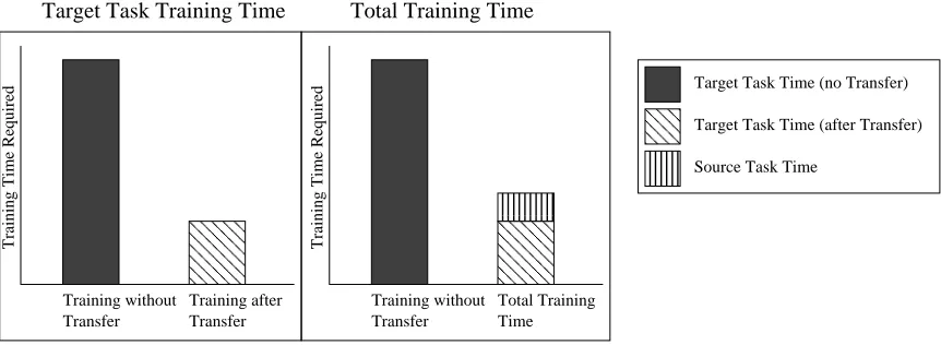
Figure 3: In this article we evaluate transfer by both considering the training time in the target task (left) and by considering the total time spent training in both tasks (right).
For these reasons we use the time-to-threshold metric. After preliminary experiments are con-ducted, thresholds for analysis are chosen such that all trials must learn for some amount of time before reaching the performance threshold, and most trials are able to eventually reach the thresh-old. We will show in Section 6 that given a Q(source,f inal), the training time for the learner in the target task to reach some performance threshold decreases when initializing Q(target,initial) with
ρ(Q(source,f inal)). This criterion is relevant when the source task is given and is of interest in its
A stronger measure of success that we will also use is that the training time for both tasks using
TVITMis shorter than the training time to learn just the target task without transfer. This criterion is relevant when the source task is created for the sole purpose of speeding up learning with transfer and Q(source,f inal)is not reused.
3. Testbed Domains
This section introduces the Keepaway task, the testbed domain where we empirically evaluate our transfer method, and use as a running example throughout the rest of the article. We also introduce the Knight Joust, a task which we will later use as a supplemental source task from which to transfer into Keepaway.
3.1 The Keepaway Task
RoboCup simulated soccer is well understood, as it has been the basis of multiple international competitions and research challenges. The multiagent domain incorporates noisy sensors and actu-ators, as well as enforcing a hidden state so that agents only have a partial world view at any given time. While previous work has attempted to use machine learning to learn the full simulated soccer problem (Andre and Teller, 1999; Riedmiller et al., 2001), the complexity and size of the problem have so far proven intractable. However, many of the RoboCup subproblems have been isolated and solved using machine learning techniques, including the task of playing Keepaway. By focusing on the smaller task of Keepaway we are able to use reinforcement learning to learn an action-value function for a more complex task, establish thatTVITMprovides considerable benefit, and hold the
required computational resources to manageable levels.
Since late 2002, the Keepaway task has been part of the official release of the open source RoboCup Soccer Server used at RoboCup (starting with version 9.1.0). Agents in the simulator (Noda et al., 1998) receive visual perceptions every 150 msec indicating the relative distance and angle to visible objects in the world, such as the ball and other agents. They may execute a primitive, parameterized action such asturn(angle),dash(power), orkick(power,angle)every 100 msec. Thus the agents must sense and act asynchronously. Random noise is injected into all sensations and actions. Individual agents must be controlled by separate processes, with no inter-agent com-munication permitted other than via the simulator itself, which enforces comcom-munication bandwidth and range constraints. Full details of the simulator are presented in the server manual (Chen et al., 2003).
When started in a special mode, the simulator enforces the rules of the Keepaway task, as described below, instead of the rules of full soccer. In particular, the simulator places the players at their initial positions at the start of each episode and ends an episode when the ball leaves the play region or is taken away. In this mode, the simulator also informs the players when an episode has ended and produces a log file with the duration of each episode.
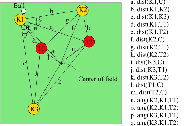
are all adjustable. This paper will use standard settings with the exception of a set of experiments in Section 7.1 that uses different kick speed actuators. Figure 4 shows a diagram of 3 keepers and 2 takers (3 vs. 2).1
b. dist(K1,K2) c. dist(K1,K3) d. dist(K1,T1) e. dist(K1,T2) f. dist(K2,C) g. dist(K2.T1) h. dist(K2,T2) i. dist(K3,C) j. dist(K3,T1)
l. dist(T1,C) m. dist(T2,C) n. ang(K2,K1,T1) o. ang(K2,K1,T2) p. ang(K3,K1,T1) q. ang(K3,K1,T2) Ball
K1
K2
T1
K3
a. dist(K1,C) b
d e
g
k. dist(K3,T2) c
j l
a
T2
k i
m h f
Center of field q no
p
Figure 4: This diagram depicts the distances and angles used to construct the 13 state variables used for learning with 3 keepers and 2 takers. Relevant objects are the 5 players and the center of the field, C. All 13 state variables are enumerated later in Table 1.
When Keepaway was introduced as a testbed (Stone and Sutton, 2002), a standard task was defined. All our experiments are run on a code base derived from version 0.6 of the benchmark Keepaway implementation2(Stone et al., 2006) and the RoboCup Soccer Server version 9.4.5.
Our setup is similar to past research in Keepaway (Stone et al., 2005), which showed that Sarsa with CMAC function approximation can learn well in this domain. On a 25m×25m field, three keepers are initially placed near three corners of the field and a ball is placed near one of the keepers. The two takers are placed in the fourth corner. When the episode starts, the three keepers attempt to keep control of the ball by passing among themselves and moving to open positions. The keeper with the ball has the option to either pass the ball to one of its two teammates or to hold the ball. In this task A ={hold, pass to closest teammate, pass to second closest teammate}. S is defined by 13 state variables, as shown in Figure 4. When a taker gains control of the ball or the ball is kicked out of the field’s bounds the episode is finished. The reward to the learning algorithm is the number of time steps the ball remains in play after an action is taken. After an episode ends, the next starts with a random keeper placed near the ball.
3.2 Knight Joust
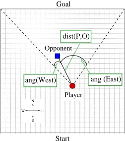
Knight Joust is a variation on a previously introduced task (Taylor and Stone, 2007) situated in the grid world domain. In this task the player begins on one end of a 25m×25m board, the opponent begins on the other, and the players alternate moves. The player’s goal is to reach the opposite
E N W
S
Start
Goal
dist(P,O)
ang(West)
ang (East)
Player
Opponent
Figure 5: Knight Joust: The player attempts to reach the goal end of a a 25×25 grid-world while the opponent attempts to touch the player.
end of the board without being touched by the opponent (see Figure 5); the episode ends if the player reaches the goal line or the opponent is on the same square as the player. The state space is discretized into 1m squares and there is no noise in the perception. The player’s state variables are composed of the distance from the player to the opponent, and two angles which describe how much of the goal line is viewable by the player.
if opponent is E of player then
Move W with probability 0.9
else if opponent is W of player then
Move E with probability 0.9
if opponent is N of player then
Move S with probability 1.0
else if opponent is S of player then
Move N with probability 0.8
The player receives a reward of+20 every time it takes the forward action, 0 if either knight jump action is taken, and an additional+20 upon reaching the goal line. The player uses Sarsa with a Q-value table to learn in this task. While this task is quite different from Keepaway, there are some similarities, such as favoring larger distances between player and opponent. This domain is much simpler than Keepaway and an agent takes roughly 20 seconds of wall-clock time (roughly 50,000 episodes) to plateau in our Java-based simulation.
4. Learning Keepaway
TVITMaims to improve learning in the target task based on prior learning in the source, and therefore a prerequisite is that both source and target tasks are learnable. In this section we outline how tasks in the Keepaway domain are learned using Sarsa.
4.1 Sarsa
Sarsa is a TD method that learns to estimate the action-value function by backing up the received rewards through time. Sarsa is an acronym for State Action Reward State Action, describing the 5-tuple needed to perform the update: (st,at,r,st+1,at+1), where st, at are the the agent’s current state and action, r is the immediate reward the agent receives from the environment, and st+1, at+1
are the agent’s subsequent state and chosen action. After each action, action values are updated according to the following rule:
Q(st,at)←(1−α)Q(st,at) +α(r+Q(st+1,at+1)) (1)
where α is the learning rate. Note that if the task is non-episodic we need to include an extra discount factor to weigh immediate rewards more heavily than future rewards.
Like other TD methods, Sarsa estimates the value of a given state-action pair by bootstrapping off the estimates of other such pairs. In particular, the value of a given state-action pair(st,at)can be estimated as r+Q(st+1,at+1), which is the value of the subsequent state-action pair(st+1,at+1)plus the immediate reward received during the transition. Sarsa’s update rule takes the old action-value estimate Q(st,at), and moves it incrementally closer towards this new estimate. The learning rate parameterαcontrols the size of these increments. Ideally, these action-value estimates will become more accurate over time and the agent’s policy will steadily improve.
4.2 Framing the RL Problem
the learners choose not from the simulator’s primitive actions but from a set of higher-level macro-actions implemented as part of the player. These macro-macro-actions can last more than one time step and the keepers have opportunities to make decisions only when an on-going macro-action terminates. To handle such situations, it is convenient to treat the problem as a semi-Markov decision process, or SMDP (Puterman, 1994; Bradtke and Duff, 1995). The agents make decisions at discrete SMDP time steps (when macro-actions are initiated and terminated).
The keepers learn in a constrained policy space: they have the freedom to decide which action to take only when in possession of the ball. A keeper in possession may either hold the ball or pass to one of its teammates. Therefore the number of actions from which the keeper with the ball may choose is equal to the number of keepers in the task. Keepers not in possession of the ball are required to execute the Receive macro-action in which the player who can reach the ball the fastest goes to the ball and the remaining players follow a handcoded strategy to try to get open for a pass. When training the keepers, the behavior of the takers is “hard-wired” and relatively simple. The two takers that are closest to the ball go directly toward it. Note that a single keeper can hold the ball indefinitely from a single taker by constantly keeping its body between the ball and the taker. The remaining takers, if present, try to block open passing lanes.
The keepers learn which action to take when in possession of the ball by using episodic SMDP Sarsa(λ) (Sutton and Barto, 1998), to learn their task.3 The episode consists of a sequence of states, macro-actions, and rewards. We choose episode duration as the performance measure for this task: the keepers attempt to maximize it while the the takers try to minimize it. Since we want the keepers to maintain possession of the ball for as long as possible, the reward in the Keepaway task is simply the number of time steps the ball remains in play after a macro-action is initiated. Learning attempts to discover an optimal action-value function that maps state-action pairs to expected time steps until the episode will end.
As more players are added to the task, Keepaway becomes harder for the keepers because the field becomes more crowded. As more takers are added there are more players to block passing lanes and chase down any errant passes. As more keepers are added, the keeper with the ball has more passing options but the average pass distance is shorter. This reduced distance forces more passes and often leads to more errors because of the noisy actuators and sensors. For this reason, keepers in 4 vs. 3 (i.e., 4 keepers and 3 takers) take longer to learn an optimal control policy than in 3 vs. 2. The average episode length of the best policy for a constant field size also decreases when adding an equal number of keepers and takers. The time needed to learn a policy with performance roughly equal to a handcoded solution roughly doubles as each additional keeper and taker is added (Stone et al., 2005). In our experiments we set the agents to have a 360◦ field of view. Although agents do also learn with a more realistic 90◦field of view, allowing the agents to see 360◦speeds up the rate of learning, enabling more experiments. Additionally, 360◦ vision also increases the learned hold times in comparison to learning with the limited 90◦vision.
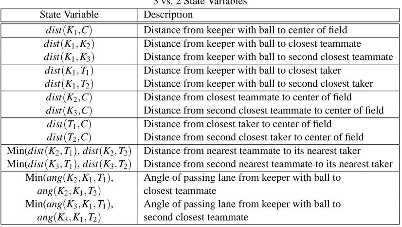
For the purposes of this article, it is particularly important to note the state variables and ac-tion possibilities used by the learners. The keepers’ states consist of distances and angles of the keepers K1−Kn, the takers T1−Tm, and the center of the playing region C (see Figure 4 and Ta-ble 1). Keepers and takers are ordered by increasing distance from the ball, leading to an indexical representation. Note that as the number of keepers n and the number of takers m increase, the num-ber of state variables also increases so that the more complex state can be fully described. S must
3 vs. 2 State Variables
State Variable Description
dist(K1,C) Distance from keeper with ball to center of field
dist(K1,K2) Distance from keeper with ball to closest teammate
dist(K1,K3) Distance from keeper with ball to second closest teammate
dist(K1,T1) Distance from keeper with ball to closest taker
dist(K1,T2) Distance from keeper with ball to second closest taker
dist(K2,C) Distance from closest teammate to center of field
dist(K3,C) Distance from second closest teammate to center of field
dist(T1,C) Distance from closest taker to center of field
dist(T2,C) Distance from second closest taker to center of field
Min(dist(K2,T1), dist(K2,T2) Distance from nearest teammate to its nearest taker
Min(dist(K3,T1), dist(K3,T2) Distance from second nearest teammate to its nearest taker
Min(ang(K2,K1,T1), Angle of passing lane from keeper with ball to
ang(K2,K1,T2) closest teammate
Min(ang(K3,K1,T1), Angle of passing lane from keeper with ball to
ang(K3,K1,T2) second closest teammate
Table 1: This table lists all state variables used for representing the state of 3 vs. 2 Keepaway. Note that the state is ego-centric for the keeper with the ball and rotationally invariant.
change (e.g., there are more distances to players to account for) and|A|increases as there are more teammates for the keeper with possession of the ball to pass to.
4.3 Function Approximation
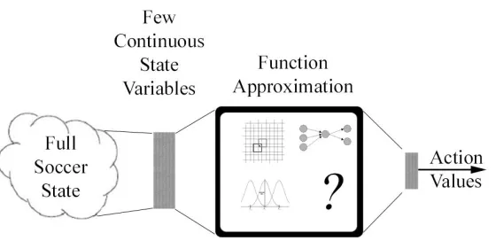
Continuous state variables combined with noise necessitate some form of function approximation for the action-value function: an agent will rarely visit the same state twice, with the possible exception of an initial start state. In this article we use three distinct function approximators and show that all are able to learn Keepaway, as well as use our transfer methodology (see Figure 6). In one implementation, we use linear tile-coding function approximation, also known as a CMAC (cerebellar model arithmetic computer), which has been successfully used in many reinforcement learning systems (Albus, 1981), including past Keepaway research (Stone et al., 2005). A second uses radial basis function approximation (RBF) (Sutton and Barto, 1998). The third implementation uses artificial neural networks (ANN), another method for function approximation that has had some notable past successes (Tesauro, 1994; Crites and Barto, 1996).
Figure 6: Function approximation is necessary for agents interacting with a continuous world. This article examines three different function approximators for Keepaway but many different methods could in principle be used by a transfer learner.
ˆ
f(x) =
∑
i
wifi(x) (2)
but only tiles which are activated by the current state feature contribute to the sum:
fi(x) =
1, if tile i is activated 0, otherwise.
By default, all the CMAC’s weights are initialized to zero. This approach to function approx-imation in the RoboCup soccer domain has been detailed previously (Stone et al., 2005). We use one-dimensional tilings so that each state variable is tiled independently, but the principles apply in the n-dimensional case. For each variable, 32 tilings were overlaid, each offset from the others by by 321 of a tile width. For each tiling, the current state activates a single tile. In 3 vs. 2, there are 32 tiles active for each state variable and 13×32=416 tiles activated in total. The tile widths are defined so that the distance state features have a width of roughly 3.0 meters and tiles for angle state features are roughly 10.0 degrees. In this work we do not vary these settings but set them to agree with past work.
RBF function approximation is a generalization of the tile coding idea to continuous functions (Sutton and Barto, 1998) and their application in Keepaway have been introduced elsewhere (Stone et al., 2006). When considering a single state variable, an RBF approximator is a linear function approximator:
ˆ
f(x) =
∑
i
wifi(x) (3)
where the basis functions have the form:
fi(x) =φ(|x−ci|) (4)
x is the value of the current state variable, ci is the center of feature i (which is unchanged from
the CMAC, Equation 2), and wi represents weights that can be modified over time by a learning algorithm. Here we set the features to be evenly spaced Gaussian radial basis functions, where:
φ(x) =exp(− x 2
The σparameter controls the width of the Gaussian function and therefore the amount of gener-alization over the state space. We set σto 0.25, which roughly spans the width of three CMAC tiles, after running experiments withσ=1.0,0.5,0.25 and observing that the learning rates were not dramatically effected.
As we did with the CMAC, we again assume that the state variables are independent and thus have one set of linearly tiled RBFs for each state variable. Similar to the CMAC implementation, all state variables are tiled independently and there are 32 tilings for each state variable. The RBFs in every tiling are spaced so that their centers correspond to the centers of CMAC tiles. We use Equations 3-5 to calculate Q-values of a state s. Because σspecifies that the spread of a RBF is roughly 3 CMAC tiles, each 3 vs. 2 state will thus be computed from approximately 3×13×32=
1248 weights in total. All weights wiare initially set to zero, but over time learning updates changes the values of the weights so that the resulting Q-values more closely predict the true returns, as specified by Equation 1.
The ANN function approximator similarly allows a learner to approximate the action-value function, given a set of continuous, real valued, state variables. Each input to the ANN is set to the value of a state variable and the output corresponds to an action. Activations of the output nodes correspond to Q values. We use a fully-connected feedforward network with a single hidden layer of 20 sigmoid units for all our tasks. The output layer nodes are linear and return the currently predicted Q(s,a)for each action. Weights were initialized with uniformly random numbers chosen from[0,1.0]. We had also tried initializing the weights uniformly to 0 and from[0,0.01], with little effect on learning rates. This network topology was selected after testing 7 different sizes of hidden layers, from 5 to 30 hidden units. Again, the learning rate did not seem to be strongly affected by this parameter. The network is trained using standard backpropagation where the error signal to modify weights is generated by the Sarsa algorithm, as with the other function approximators.
4.4 Learning 3 vs. 2 Keepaway
To learn 3 vs. 2 Keepaway as a source task for transfer, all weights in the CMAC and RBF function approximators are initially set to zero; every initial state-action value is thus zero and our action-value function is uniform. All weights and biases in the 13-20-3 feedforward ANN are set to small random numbers to encourage faster backprop training (Mehrotra et al., 1997) but the initial action-value is still nearly uniform. As training progresses, the weights of the function approximators are changed by Sarsa so that the average hold time of the keepers increases.
In our experiments we set the learning rate,α, to be 0.1 for the CMAC function approximator, as in previous experiments. αwas 0.05, and 0.125 for the RBF and ANN function approximators, respectively. These values were determined after trying approximately five different learning rates for each function approximator. The exploration rate,ε, was set to 0.01 (1%) in all experiments and
λwas set to 0, which we selected to be consistent with past work (Stone et al., 2005).
4.5 Learning 4 vs. 3 Keepaway and 5 vs. 4 Keepaway without Transfer
to second closest teammate, pass to third closest teammate}, and S is made up of 19 state variables due to the added players.
It is also important to point out that the addition of an extra taker and keeper in 4 vs. 3 results in a qualitative change in the task. In 3 vs. 2 both takers must go towards the ball as two takers are needed to capture the ball from the keeper. However, the third taker is now free to roam the field and attempt to intercept passes. This necessarily changes the keeper behavior as one teammate is often blocked from receiving a pass by this new taker. Furthermore, adding a keeper in the center of the field changes the start state significantly as now the keeper that starts with the ball has a teammate that is closer to itself, but is also closer to the takers.
In order to quantify how fast an agent in 4 vs. 3 learns, we set a target performance of 10.0 seconds for ANN learners, while CMAC and RBF learners have a target of 11.5 seconds. These threshold times are chosen so that learners are able to consistently attain the performance level without transfer, but players using TVITM must also learn and do not initially perform above the threshold. CMAC and RBF learners are able to learn better policies than the ANN learners and thus have higher threshold values. When a group of four CMAC keepers has learned to hold the ball from the three takers for an average of 11.5 seconds over 1,000 episodes we say that the keepers have sufficiently learned the 4 vs. 3 task. Thus agents learn until the on-line reward of the keepers, averaged over 1,000 episodes, with exploration, passes a set threshold.4 In 4 vs. 3, it takes a set of four keepers using CMAC function approximators 30.8 simulator hours (roughly 15 hours of wall-clock time, or 12,000 episodes) on average to learn to hold the ball for 11.5 seconds when training without transfer. By comparison, in 3 vs. 2, it takes a set of three keepers using CMAC function approximators 5.5 hours on average to learn to hold the ball for 11.5 seconds when training without transfer.
The ANN used in 4 vs. 3 is a 19-20-4 feedforward network.5The ANN learners do not learn as quickly nor achieve as high a performance before learning plateaus and therefore we use a threshold of 10.0 seconds. (After training four keepers using ANN function approximation without transfer in 4 vs. 3 for over 80 hours, the average hold time was only 10.3 seconds.)
5 vs. 4 is harder than 4 vs. 3 for the same reasons that 4 vs. 3 is more difficult than 3 vs. 2. In 5 vs. 4 three keepers are again placed in three corners and the two remaining keepers are placed in the middle of the 25m×25m field. All four takers are placed in the fourth corner. There are now five actions:{hold, pass to closest teammate, pass to second closest teammate, pass to third closest
teammate, pass to fourth closest teammate}, and 25 state variables. In 5 vs. 4, it takes a set of five
keepers using CMAC function approximators 59.9 hours (roughly 24,000 episodes) on average to learn to hold the ball for 11.5 seconds when training without transfer. In this paper we investigate the 5 vs. 4 problem only with the CMAC function approximator.
5. Transfer via Inter-Task Mapping in Keepaway
Having introduced our testbed domain and baseline learning approaches, we can now show how
TVITMis performed in Keepaway, utilizing terminology described in Section 2. Recall thatTVITM
4. We begin each trial by following the initial policy for 1,000 episodes without learning (and therefore without counting this time towards the learning time). This enables us to assign a well-defined initial performance when we begin learning because there already exist 1,000 episodes to average over.
relies on a functional ρthat is able to transfer an action-value function from a source task into a target task with different state and action spaces.ρis built from the inter-task mappingsχX andχA,
and thus this section begins by defining these two mappings and then describing how they are used to generate differentρs.
In the Keepaway domain, A and S are determined by the current Keepaway task and thus differ from instance to instance. sinitial, R, and T , though formally different, are effectively constant across tasks. When S and A change, sinitial, R, and T change by definition because they are functions defined over S and A, but in practice R is always defined as+1 for every time step that the keepers maintain possession, and sinitialand T are always defined by the RoboCup soccer simulation.
5.1 DefiningχX andχA for 4 vs. 3 Keepaway and 3 vs. 2 Keepaway
In the Keepaway domain we are able to intuit the inter-task mappings between states and actions in the two tasks based on our knowledge of the domain. Our choice for the mappings is supported by empirical evidence in Section 6 showing that using these mappings do allow us to construct transfer functions that successfully reduce training time. In general, the transform may not be so straightforward, but experimenting in a domain where it is easily defined allows us to focus on showing the benefits of transfer. This article demonstrates that transfer can be successful when a mapping is available, while we leave it to future work to show how to best construct (or learn) such a transform.
We define χA, the inter-task mapping between actions in the two tasks, by identifying actions
that have similar effects on the world state in both tasks. For the 3 vs. 2 and 4 vs. 3 tasks, the action “Hold ball” is equivalent because this action has a similar effect on the world in both tasks. Likewise, the action “Pass to closest keeper” is analogous in both tasks, as is “Pass to second closest keeper.” We map the novel target action “Pass to third closest keeper” to “Pass to second closest keeper” in the source task.
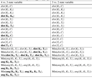
The state variable mapping,χX, is handled with a similar strategy. Each of the 19 state variables in the 4 vs. 3 task is mapped to a similar state variable in the 3 vs. 2 task. For instance, “Distance to closest keeper” is the same in both tasks. “Distance to second closest keeper” in the target task is similar to “Distance to second closest keeper” in the source task. “Distance to third closest keeper” in the target task is also mapped to “Distance to second closest keeper” in the source task. See Table 2 for a full description ofχX.
Now that χA andχX are defined, relating the state variables and actions in a target task to the state variables and actions in a source task, we can use them to constructρs for different internal representations. The functionals will transfer the learned action-value function from the source task into the target task. We denote these functionals asρCMAC,ρRBF, andρANN for the CMAC, RBF, and ANN function approximators, respectively.
5.2 DefiningχX andχA for 4 vs. 3 Keepaway and Knight Joust
Description ofχX Mapping from 4 vs. 3 to 3 vs. 2
4 vs. 3 state variable 3 vs. 2 state variable
dist(K1,C) dist(K1,C)
dist(K1,K2) dist(K1,K2)
dist(K1,K3) dist(K1,K3)
dist(K1,K4) dist(K1,K3)
dist(K1,T1) dist(K1,T1)
dist(K1,T2) dist(K1,T2)
dist(K1,T3) dist(K1,T2)
dist(K2,C) dist(K2,C)
dist(K3,C) dist(K3,C)
dist(K4,C) dist(K3,C)
dist(T1,C) dist(T1,C)
dist(T2,C) dist(T2,C)
dist(T3,C) dist(T2,C)
Min(dist(K2,T1), dist(K2,T2), dist(K2,T3)) Min(dist(K2,T1), dist(K2,T2))
Min(dist(K3,T1), dist(K3,T2), dist(K3,T3)) Min(dist(K3,T1), dist(K3,T2))
Min(dist(K4,T1), dist(K4,T2), dist(K4,T3)) Min(dist(K3,T1), dist(K3,T2))
Min(ang(K2,K1,T1), ang(K2,K1,T2), Min(ang(K2,K1,T1), ang(K2,K1,T2)) ang(K2,K1,T3))
Min(ang(K3,K1,T1), ang(K3,K1,T2), Min(ang(K3,K1,T1), ang(K3,K1,T2)) ang(K3,K1,T3))
Min(ang(K4,K1,T1), ang(K4,K1,T2), Min(ang(K3,K1,T1), ang(K3,K1,T2)) ang(K4,K1,T3))
Table 2: This table describes the mapping between states in 4 vs. 3 to states in 3 vs. 2. The distance between a and b is denoted as dist(a,b); the angle made by a, b, and c, where b is the vertex, is denoted by ang(a,b,c); and values not present in 3 vs. 2 are in bold. Relevant points are the center of the field C, keepers K1-K4, and takers T1-T3, where players are
ordered by increasing distance from the ball.
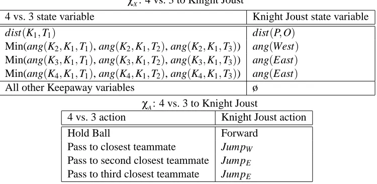
Table 3 describes the inter-task mappings used to transfer between Knight Joust and 4 vs. 3 Keepaway. Our hypothesis was that the Knight Joust player would learn to move North when pos-sible and jump to the side when necessary, which could be similar to holding the ball in Keepaway when possible and passing when necessary.
5.3 ConstructingρCMACandρRBF
The CMAC function approximator takes a state and an action and returns the expected long-term reward. The learner can evaluate each possible action for the current state and then useπto choose one. We construct aρCMACand use it so that when the learner considers a 4 vs. 3 action, the weights for the activated tiles are not zero but instead are initialized by Q(3vs2,f inal). To accomplish this, we copy weights learned in the source CMAC into weights in a newly initialized target CMAC, using
χX: 4 vs. 3 to Knight Joust
4 vs. 3 state variable Knight Joust state variable
dist(K1,T1) dist(P,O)
Min(ang(K2,K1,T1), ang(K2,K1,T2), ang(K2,K1,T3)) ang(West)
Min(ang(K3,K1,T1), ang(K3,K1,T2), ang(K3,K1,T3)) ang(East)
Min(ang(K4,K1,T1), ang(K4,K1,T2), ang(K4,K1,T3)) ang(East)
All other Keepaway variables ø
χA: 4 vs. 3 to Knight Joust
4 vs. 3 action Knight Joust action
Hold Ball Forward
Pass to closest teammate JumpW Pass to second closest teammate JumpE Pass to third closest teammate JumpE
Table 3: This table describes the mapping between state variables and actions from 4 vs. 3 to Knight Joust. Note that the we have made Jump West in the Knight Joust correspond to passing to K2 and Jump East correspond to passing to K3, but either is reasonable, as long as the
state variables and actions are consistent.
Note that this target CMAC will initially be unable to distinguish between some states and actions because the inter-task mappings allow duplication of values. For instance, the weights corresponding to the tiles that are activated for the “Pass to second closest teammate” in the source task are copied into the weights for the tiles that are activated to evaluate the “Pass to second closest teammate” action and the “Pass to third closest teammate” in the target task. The 4 vs. 3 agents are initially unable to distinguish between these two actions. In other words, because the values for the weights corresponding to the two 4 vs. 3 actions are the same, Q(4vs3,initial)will evaluate both actions as having the same expected return. The 4 vs. 3 agents will therefore have to learn to differentiate these two actions as they learn in the target task.
Algorithm 1 APPLICATION OFρCMAC
1: for each non-zero weight, wi in the source CMAC do
2: xsource←value of state variable corresponding to tile i
3: asource←action corresponding to i
4: for each value xtargetsuch thatχX(xtarget) =xsourcedo 5: for each value atarget such thatχA(atarget) =asourcedo 6: j←the tile in the target CMAC activated by xtarget,atarget
7: wj←wi
8: wAverage←average value of all non-zero weights in the target CMAC
9: for each weight wjin the target CMAC do
10: if wj=0 then
As a final step (Algorithm 1, lines 8–11), any weights which have not been initialized byρCMAC are set to the average value of all initialized weights. The 3 vs. 2 training was likely not exhaustive and therefore some weights which may be used in 4 vs. 3 would otherwise remain uninitialized. Tiles which correspond to every value in the new 4 vs. 3 state vector have thus been initialized to values determined via training in 3 vs. 2 and can therefore be considered in the computation. This averaging effect is discussed further in Section 6 and has the effect of allowing agents in the target task to learn faster.
ρRBF is constructed similarly to ρCMAC. The main difference between the RBF and CMAC function approximators are how weights are summed together to produces values, but the weights have similar structure in both function approximators. For a given state variable, a CMAC sums one weight per tiling. An RBF differs in that it sums multiple weights for each tiling, where weights are multiplied by the Gaussian functionφ(x−ci). Thus when usingρRBF we copy weights following the same schema as inρCMACin Algorithm 1.
5.4 ConstructingρANN
To construct a (fully connected, feedforward) neural network for the 4 vs. 3 target task, the 13-20-3 network from 3 vs. 2 is first augmented by adding 6 inputs and 1 output node. The weights connecting inputs 1–13 to the hidden nodes are copied over from the 13-20-3 network. Likewise, the weights from hidden nodes to outputs 1–3 are copied over to the 19-20-4 network. Weights from inputs 14-19 to the hidden nodes correspond to the new state variables and are copied over from the analogous 3 vs. 2 state variable, according toχX. The weights from the hidden nodes to the novel
output are copied over from the analogous 3 vs. 2 action, according toχA. Every weight in the 19-20-4 network is therefore set to an initial value based on the trained 13-20-3 network. Algorithm 2 describes this process in detail. We define the functionψto map nodes in the two networks:
ψ(n) =
χX(n), if n is an input
χA(n), if n is an output
δ(n), if n is a hidden node
where a functionδrepresents the correspondence between these hidden nodes (δ(htarget) =hsource). In our case the number of hidden nodes used are the same in both tasks. Therefore, in practice
ψ(“nthhidden node in the source network”) = “nthhidden node in the target network.”
Whereas ρCMAC andρRBF copied many weights (hundreds or thousands, where increasing the amount of 3 vs. 2 training will increase the number of learned non-zero weights), ρANN always copies the same number of weights regardless of training. In fact, ρANN initializes only 140 new weights (in addition to the 320 weights that existed in 3 vs. 2) in the 4 vs. 3 representation and is therefore in some sense simpler than the otherρs.
Algorithm 2 APPLICATION OFρANN
1: for each pair of nodes ni,njin ANNtargetdo
2: if link(ψ(ni),ψ(nj)) exists in ANNsourcethen
5.5 Q-value Reuse
The threeρs previously introduced are specific to particular function approximators. In this section we introduce a different approach, Q-value Reuse, to transfer between a source and target. Rather than initialize a function approximator in the target task with values learned in the source task, we instead reuse the entire learned source task’s Q-values. A copy of the source task’s function approximator is retained so that it can calculate the source task’s Q-values for any state, action pair: QsourceFA: S×A7→R. When computing Q-values for the target task, we first map the target task state and action to the source task’s state and action via the inter-task mappings. The computed Q-value is a combination of the output of the source task’s saved function approximator and the target task’s current function approximator:
Q(s,a) =QsourceFA(χX(s),χA(a)) +QtargetFA(s,a)
Sarsa updates in the target task are computed as normal, but only the target function approximator’s weights are eligible for updates. Note that ifχX(s)orχA(a)were undefined for a certain s,a pair in
the target task, Q(s,a)would equal QtargetFA(s,a).
Q-value Reuse may be considered a type of reward shaping (Colombetti and Dorigo, 1993; Mataric, 1994): we are able to directly use the expected rewards from the source task to bias the learner in the target task. This method has two advantages. First, it is not function-approximator specific, and could, in theory, be used to transfer between different function approximators as well as between different tasks. Second, there is no initialization step needed between learning the two tasks. However, drawbacks include an increased lookup time and larger memory requirements. Such requirements will grow linearly in the number of transfer steps; while they are not substantial with a single source task, they may become prohibitive when using multiple source tasks or when performing doing multi-step transfer (such as shown later in Section 7.2).
6. Experimental Results: 3 vs. 2 Keepaway to 4 vs. 3 Keepaway
This section discusses the results of our transfer experiments between the 3 vs. 2 and 4 vs. 3 Keep-away tasks using our two metrics, training time reduction in the target task and total training time reduction. Section 6.1 shows the success of transfer when the 3 vs. 2 is used as a source task to learn 4 vs. 3. Section 6.2 includes additional analysis of these results. Section 6.3 demonstrates transfer between 3 vs. 2 and 4 vs. 3 CMAC players using Q-value Reuse.
6.1 Transferring viaρfrom 3 vs. 2 Keepaway into 4 vs. 3 Keepaway
Having constructed three ρs that transform the learned action-value functions, we can now set Q(4vs3,initial) = ρ(Q(3vs2,f inal)) between Keepaway agents with CMAC, RBF, or ANN function ap-proximation. We do not claim that these initial action-value functions are correct (and empirically they are not), but instead that the constructed action-value functions allow the learners to more quickly discover a better-performing policy.
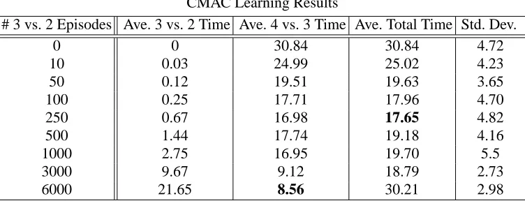
CMAC Learning Results
# 3 vs. 2 Episodes Ave. 3 vs. 2 Time Ave. 4 vs. 3 Time Ave. Total Time Std. Dev.
0 0 30.84 30.84 4.72
10 0.03 24.99 25.02 4.23
50 0.12 19.51 19.63 3.65
100 0.25 17.71 17.96 4.70
250 0.67 16.98 17.65 4.82
500 1.44 17.74 19.18 4.16
1000 2.75 16.95 19.70 5.5
3000 9.67 9.12 18.79 2.73
6000 21.65 8.56 30.21 2.98
Table 4: Results showing that learning Keepaway with a CMAC and applying transfer via inter-task mapping reduces training time (in simulator hours) for CMAC players. Minimum learning times for reaching the 11.5 second threshold are bold. As source task training time increases, the required target task training time decreases. The total training time is minimized with a moderate amount of source task training.
threshold performance levels6show that agents utilizing CMAC, RBF, and ANN function approxi-mation are all able to learn faster in the target task by usingρCMAC,ρRBF, andρANN, respectively.
Tables 4 and 5 show learning times to reach a threshold performance and verify that a CMAC, an RBF, and an ANN successfully allow independent players to learn to hold the ball from opponents when learning without transfer; agents utilizing these three function approximation methods are able to successfully attain the 4 vs. 3 threshold performance.7
This result shows that a CMAC is more efficient than an ANN trained with backprop, another obvious choice. We posit that this difference is due to the CMAC’s property of locality. When a particular CMAC weight for one state variable is updated during training, the update affects the output value of the CMAC for other nearby state variable values. The width of the CMAC tiles determines the generalization effect and outside of this tile width, the change has no effect. Contrast this with the non-locality of an ANN. Every weight is used for the calculation of an action-value function, regardless of how close two inputs are in state space. Any update to a weight in the ANN must necessarily change the final output of the network for every set of inputs. Therefore it may take the ANN longer to settle into an effective configuration. Furthermore, the ANNs use many fewer weights than the CMAC and RBF learners, which may have allowed for faster learning at the cost of reduced performance of the final policy.
The RBF function approximator had the best performance of the three when learning without transfer (i.e., the top row of each table). The RBF shares the CMAC’s locality benefits, but is also able to generalize more smoothly due to the Gaussian summation of weights.
To test the effect of using transfer with a learned 3 vs. 2 action-value function, we train a set of keepers for a number of 3 vs. 2 episodes, save the function approximator’s weights (Q(3vs2,f inal))
6. Our results hold for other threshold times as well, provided that the threshold is not initially reached without training and that learning will enable the keepers’ performance to eventually cross the threshold.
0 5 10 15 20 25 30
10 100 1000
Simulator Hours to Achieve
Threshold Performance
# of 3 vs. 2 Episodes CMAC Learning Results
0 5 10 15 20 25 30
10 100 1000
Simulator Hours to Achieve
Threshold Performance
# of 3 vs. 2 Episodes CMAC Learning Results
0 5 10 15 20 25 30
10 100 1000
Simulator Hours to Achieve
Threshold Performance
# of 3 vs. 2 Episodes CMAC Learning Results
4 vs. 3 time 3 vs. 2 time Baseline time: no transfer
Figure 7: A graph of Table 4 where the x-axis uses a logarithmic scale. The thin bars show the amount of time spent training in the source task, the thick bars show the amount of time spent training in the target task, and their sum represents the total time. The target task training time is reduced as more time is spent training in the source task. The total time is minimized when using a moderate amount of source task training.
from a random 3 vs. 2 keeper, and use the weights to initialize all four keepers8 in 4 vs. 3 so that Q(4vs3,initial)←ρ(Q(3vs2,f inal)). Then we train on the 4 vs. 3 Keepaway task until the average hold time for 1,000 episodes is greater than some performance threshold. Recall that in section 4.5 we specify a threshold of 11.5 seconds in the case of CMAC and RBF function approximators and 10.0 seconds for ANNs as neural network agents were unable to learn as effectively.
To determine if Keepaway players using CMAC function approximation can benefit from trans-fer, we compare the time it takes agents to learn the target task after transferring from the source task with the time it takes to learn the target task without transfer. The result tables show different amounts of source task training time, where the minimal learning times are in bold. The top row of each table represents learning the task without transfer and thus any column with transfer times lower than the top row shows beneficial transfer. Our second goal of transfer would be met if the total training time in both tasks with transfer was less than learning without transfer in the target task. Table 4 reports the average time spent training in 4 vs. 3 with CMAC function approximation to achieve an 11.5 second average hold time after different amounts of 3 vs. 2 training. Column two reports the time spent training on 4 vs. 3 while the third column shows the total time to train 3 vs. 2 and 4 vs. 3. As can be seen from the table, spending time training in the simpler 3 vs. 2 domain can cause the learning time for 4 vs. 3 to decrease. To overcome the high amounts of noise in our evaluation we run at least 25 independent trials for each data point reported.
RBF and ANN Learning Results
# of 3 vs. 2 Ave. RBF Ave. RBF Standard Ave. ANN Ave. ANN Standard Episodes 4 vs. 3 Time Total Time Deviation 4 vs. 3 Time Total Time Deviation
0 19.52 19.52 6.03 33.08 33.08 16.14
10 18.99 19.01 6.88 19.28 19.31 9.37
50 19.22 19.36 5.27 22.24 22.39 11.13
100 18.00 18.27 5.59 23.73 24.04 9.47
250 18.00 18.72 7.57 22.80 23.60 12.42
500 16.56 18.12 5.94 19.12 20.73 8.81
1,000 14.30 17.63 3.34 16.99 20.19 9.53
3,000 14.48 26.34 5.71 17.18 27.19 10.68
Table 5: Results from learning Keepaway with different amounts of 3 vs. 2 training time (in simu-lator hours) indicates thatρRBF andρANN can reduce training time for RBF players (11.5 second threshold) and ANN players (10.0 second threshold). Minimum learning times for each method are in bold.
The potential ofTVITMis evident in Table 4 and Figure 7. To analyze these results, we conduct a number of Student’s t-tests to determine if the differences between the distributions of learning times for the different settings are significant. These tests confirm that the differences in the distributions of 4 vs. 3 training times when usingTVITMare statistically significant (p<0.05) when compared to training 4 vs. 3 without transfer. Not only is the time to train the 4 vs. 3 task decreased when we first train on 3 vs. 2, but the total training time is less than the time to train 4 vs. 3 without transfer. We can therefore conclude that in the Keepaway domain, training first on a simpler source task can increase the rate of learning enough that the total training time is decreased when using a CMAC function approximator. It is not obvious how to choose the amount of time to spend learning the source task to minimize the total time and this an optimization will be left for future work (see Section 8).
Analogous experiments for Keepaway players using RBF and neural network function approx-imation are presented in Table 5. Again, successful transfer is demonstrated as both the transfer agents’ target task training time and the transfer agent’s total training time are less than the time required to learn the target task without transfer. All numbers reported are averaged over at least 25 independent trials; both 4 vs. 3 time and total time can be reduced withTVITM. For the RBF players, allTVITM4 vs. 3 results using at least 500 3 vs. 2 episodes show a statistically significant difference from those that learn without transfer (p<0.05), while the learning trials that used less than 500 source task episodes did not significantly reduce the target task training time. The difference in all 4 vs. 3 training times for the ANN players between using TVITMand training without transfer is statistically significant (p<0.05).
The RBF function approximator yielded the best learning rates for 3 vs. 2 Keepaway, followed by the CMAC function approximator, and lastly the ANN trained with backpropagation. However,
Ablation Studies withρCMAC
Transfer # of 3 vs. 2 Ave. 4 Standard
Functional Episodes vs. 3 Time Deviation
No Transfer 0 30.84 4.72
ρCMAC 100 17.71 4.70
ρCMAC 1000 16.95 5.5
ρCMAC 3000 9.12 2.73
ρCMAC,No Averaging 100 25.68 4.21
ρCMAC,No Averaging 3000 9.53 2.28
only averaging 100 19.06 6.85
only averaging 3000 10.26 2.42
ρCMAC,Ave Source 1000 15.67 4.31
Table 6: Results showing that transfer with the fullρCMAC outperforms usingρCMAC without the final averaging step, using only the averaging step ofρCMAC, and when averaging weights in the source task before transferring the weights.
technique, and that more training in the source task generally reduces the time needed to learn the target task.
6.2 UnderstandingρCMAC’s Benefit
To better understand howTVITMusesρCMACto reduce the required training time in the target task, and to isolate the effects of its various components, this section details a number of supplemental experiments.9
To help understand howρCMACenables transfer we isolate its two components. We first ablate the functional so that the final averaging step (Algorithm 1, lines 8–11), which places the average weight into all zero weights, is removed. We anticipated that the benefit from transfer would be increasingly degraded, relative to using the actual ρCMAC, as fewer numbers of training episodes in the source task were used. The resulting 4 vs. 3 training times were all shorter than training without transfer, but longer than when the averaging step was incorporated. The relative benefit of our ablated ρCMAC is greater after greater numbers of source task episodes; the averaging step appears to have given initial values to weights in the state/action space that have never been visited with low numbers of source episodes and thus imparts some bias in the target task even with very little 3 vs. 2 training. Over time more of the state space in the source task is explored and thus our ablated functional performs quite well. This result shows that the averaging step is most useful with less source task training, but becomes less so as more source experience is accumulated (see Table 6 for result details).
If we perform only the averaging step fromρCMACon learners trained in the target task, we can determine how important this step is to our method’s effectiveness. Applying the averaging step
Time required for CMAC 4 vs. 3 players to reach 11.5 sec. hold time
Initial CMAC weight Ave. Learning Time Standard Deviation
0 30.84 4.72
0.5 35.03 8.68
1.0 N/A N/A
Each weight randomly selected from
the uniform distribution from [0,1.0] 28.01 6.93
Table 7: 10 independent trials are averaged for different values for initial CMAC weights. None of the trials with initial weights of 1.0 were able to reach the 11.5 threshold within 45 hours, and thus are shown as N/A above.
causes the total training time to decrease below that of training 4 vs. 3 without transfer, but again the training times are longer than runningρCMAC on weights trained in 3 vs. 2. This result confirms that both parts ofρCMAC contribute to reducing 4 vs. 3 training time and that training on 3 vs. 2 is more beneficial for reducing the required 4 vs. 3 training time than training on 4 vs. 3 and applying
ρCMAC(see Table 6 for result details).
The averaging step inρCMACis defined so that the average weight in the target CMAC overwrites all zero-weights. We also conducted a set of 30 trials which modifiedρCMAC so that the average weight in the source CMAC is put into all zero-weights in the target CMAC, which is possible when agents in the source task know that their saved weights will be used for TVITM. Table 6 shows that when the weights are averaged in the source task (ρCMAC,Ave Source) the performance is not statistically different (p<0.05 fromTVITMwhen averaging in the target task (See Table 4).
To verify that the 4 vs. 3 CMAC players were benefiting from TVITM and not from having
non-zero initial weights, we initialized CMAC weights uniformly to 0.5 in one set of experiments, 1.0 uniformly in a second set of experiments, and then to random numbers uniformly distributed from 0.0-1.0 in a third set of experiments. We do so under the assumption that 0.0, 0.5, and 1.0 are all reasonable initial values for weights (although in practice 0.0 is most common). The learning time was never statistically better than learning with weights initialized to zero, and in some experi-ments the non-zero initial weights decreased the speed of learning. Haphazardly initializing CMAC weights may hurt the learner but systematically setting them throughTVITMis beneficial. Thus we conclude that the benefit of transfer is not a byproduct of our initial setting of weights in the CMAC (see Table 7 for result details).
To further test the sensitivity of theρCMACfunction, we change it in two different ways. We first definedρmodi f ied by modifyingχA so that instead of mapping the novel target task action “Pass to
second third keeper” into the action “Pass to second closest keeper,” we instead map the novel action into “Hold ball.” Now Q4vs3,initial will initially evaluate “pass to third closest keeper” and “hold ball” as equivalent for all states. Second, we modifyχA andχX so that state variables and actions not present in 3 vs. 2 are not initialized in the target task. Using these new inter-task mappings, we constructρ3vs2, a functional which copies over information learned in 3 vs. 2 exactly but assigns the
average weight to all novel state variables and actions in 4 vs. 3.
When using this ρmodi f ied to initialize weights in 4 vs. 3, the total training time increased rel-ative to the normalρCMAC but still outperformed training without transfer. Similarly,ρ3vs2 is able