Published online December 24, 2014 (http://www.sciencepublishinggroup.com/j/pamj) doi: 10.11648/j.pamj.s.2014030602.16
ISSN: 2326-9790 (Print); ISSN: 2326-9812 (Online)
Integral geometry and complex space-time cohomology in
field theory
Francisco Bulnes
1, *, Ronin Goborov
21
Head of Research Department in Mathematics and Engineering, TESCHA, Chalco, Mexico 2
Department of Mathematics, Lomonosov University, Moscu, Russia
Email address:
[email protected] (F. Bulnes), [email protected] (R. Goborov)
To cite this article:
Francisco Bulnes, Ronin Goborov. Integral Geometry and Complex Space-Time Cohomology in Field Theory. Pure and Applied Mathematics Journal. Special Issue: Integral Geometry Methods on Derived Categories in the Geometrical Langlands Program.
Vol. 3, No. 6-2, 2014, pp. 30-37. doi: 10.11648/j.pamj.s.2014030602.16
Abstract:
Through of a cohomological theory based in the relations between integrating invariants and their different differential operators classes in the field equations as well as of functions inside of the integral geometry are established equivalences among cycles and co-cycles of the closed sub-manifolds, line bundles and contours of the space-time modeled as complex Riemannian manifold obtaining a cohomology of general integrals useful in the evaluation and measurement of fields, particles and physical interactions of diverse nature in field theory. Also are used embeddings of cycles in the complex Riemannian manifold through of the dualities: line bundles with cohomological contours and closed sub-manifolds with cohomological functional to build cohomological spaces of integrals as solution classes of the corresponding field equations.Keywords:
Complex Cohomology, Cohomology of Cycles, Cohomological Functional, Integral Operator Cohomology, Integrating Invariants, Integral Topology, Cohomological Classes1. Introduction
To can to obtain a cohomology of general integral operators that determines complex analytic solutions through classes of a cohomology that born from the ∂−cohomology is necessary to use a holomorphic language [1] with the purpose of obtain holomorphic forms that involve exact forms. In fact, this methodology is a way of so many that suggests the use of complex hyper-holomorphic functions in approach of functions in complex analysis, although using fibrations on some quaternionic algebra. The holomorphic forms required in this language are good to express the integral of complex vector field as integral of line it has more than enough lines bundles and hyperplanes like for example, having more than enough lines and hyperplanes respectively in CPn,and Cn, visualizing these fields like holomorphic sections of complex holomorphic bundles of fibrations X →M .
The ∂−cohomology exists naturally in coverings of Stein
M
X → , like holomorphic forms. Then the integral can be expressed on spaces Mδ,and ∆z[2, 3], that are lines and hyperplanes of
CP
n,
andC
n,
and that as such, they are“integral orbits” of the complex manifolds M=G/L, and
, /Σ Γ =
∆ belonging to a ∂− cohomology in holomorphic language.
The cohomologies of functional and functions respectively, can be constructed through the complex cohomology of hyper-spaces they are generalizable for vector fields in the same sense of the Stein coverings and therefore of the∂− cohomology. Then the following question arises, how to establish an isomorphism of cohomological classes for functions, functional and vector fields inside the holomorphic context possible?
Is possible to determine a cohomological theory of integral operators that establishes equivalences among these objects and the geometrical objects of closed submanifolds, bundle of lines and Feynman diagrams?
Is possible that everything can decrease to a single cohomology of general integrals on contours or cohomology of generalized functional?
Before, to give an answer to the previous questions, we give some preliminary definitions that we will use to fix concepts and outlines of the wanted general theory.
Def. 1. 1. We say that a spaceH•(M,ℑ), is an integral
operator cohomology (in the sense of the integrals of the field equations) of those ∂−equations, if this is a solution class or general integral of these equations in M [2, 4].
Def. 1. 2. An integral as generalized solution of a ∂− equation is a realization of an irreducible representation of a
−
∂ cohomology of complex closed submanifolds [3, 5]. If the irreducible representations are unitary then we have a
complex L2− cohomology or ∂− cohomology with
coefficients in the space L2. The integral operators belonging to their integral operator cohomology are those of the complex Fourier analysis.
In the case of a real reductive Lie group, the generalized integrals come determined by their orbital integrals. Let G , be a real form of G , and P , their parabolic subgroup. The C
generalized integrals in G , are the integrals on open orbits of the generalized flag manifold G /C P.
Of this way, if G=U( n1, ), and the generalized flag manifold is then
P
n, then the group of positive lines P+,(which is an U( n1, )−orbit) is an open orbit in Pn(C). In this case the integrals of line are of John type [1]:
, p , f )
p
( =
∫
L⊂ ( ) ∀ ∈R4C Pn
φ (1.1)1
The general integral in this case comes given by the twistor transform on the corresponding homogeneous lines bundle, that is to say,
)), 2 n ( O *, ( H )) 2 n ( O , (
H1 P+ − − → 1 P+ − (1.2)
Through the twistor transform like intertwining operator of induced tempered representations on a ∂−cohomology we have representations of SU(2,2) , that are orbits of a fundamental unitary (g,K)−module [4]2. Then we can to assign a vector bundle of lines with a unitary representation that classify it.
The concepts of general integral and generalized integral are different, because one refers to the whole class of solution cohomology of those ∂−equations about a complex analytic manifold and the other one refers to the classes of solution cohomology on cycles or co-cycles of the complex manifold [1, 2].
Another example in the sense of recovery of a functions space mainly the space M , is the recovering of real functions
in the space Rn, through values of certain integral operators.
Such is the case of the formula of f(x), recovered on
R
n,1 Solutions to the ultra-hyperbolic wave equation.
2 These orbits possibly are orbits of the unitary group related with electrodynamics and torsion in the space-time.
), ( ] d )} x , ( ){ , ( f [ c ) x (
f
∫ ∫
ξ λ λ ξ n λω ζΓ
− +∞
∞ −
∧ −
= (1.3)
Where the integral on λ, is understood in terms of their regularization (roll that carries out the Hilbert transform). The constant
c
, depends on the parity of the dimension of thespace Rn, where was carried the tomography [1].
To answer the first question, we need a structure of complexes that induces isomorphism in an integral operator cohomology such and as we want.
Def. 1. 3. A covering of Stein is a set of Stein manifolds
δ
M , and Ξz, of the corresponding fibers X →M , and
Ξ →
X , of the double fibration [2].
Let us consider the complexes given in [2], and let us consider the structure defined by a Stein covering given by the set of open {Mδ}, and {Ξz}, in the topology
{
(z, ) M X M ( M z )}
,X =
ξ
∈ ×Ξ ⊂ ×Ξ⇔ δ ∩Ξ ≠∅τ
(1.4)Then a complex in
X
, is the space such {Ωrh}, that forany complex {Ωr}, in a corresponding long succession having that
}, { }
{Ωrh Ωr (1.5)
that is to say, all the subcomplexes Ωrh, of the complex Ωr.
Then the integral operators cohomology H•(M,ℑ),in a complex manifold M , is that whose complexes conform a holomorphic structure that induces (in the corresponding integral manifold) a generalized according structure of integral submanifolds.
The integral submanifolds represent solutions of those ∂− equations in cycles of M . The integral submanifolds are the
corresponding cycles of M , low the integral operators of
) , ( ℑ •
M
H .
For example, if we take the complex manifold M , like a
manifold of rational curves E , about a twistor manifold z T
(where should understand each other this manifold T , like the manifold of integral submanifolds (locally)) this comes
from a projective structure of their line of E , guided z
according to the vectors in TzM , that corresponds there to the
sections of a normal bundle NEz, of the curve (infinitesimal deformations to the curve) that is to say, these conform the holomorphic structure that will induce the corresponding and according structure (that is to say, in the corresponding integral manifold). In this case the generalized according structure of integral submanifolds is the V(k) −conformal integrable structure given by T . The integral operators cohomology in this case is the given by the family of rational curves.
cohomology is H•(M,ℑ)=H0(T,O(k)).
This example is interesting not only for the fact of to be defining the integral operator cohomology that defines “integrals” to M , under conditions of their proper complex differentiable structure, also for the fact of satisfy the integrability condition for the equation of the Weyl tensor
, 0
=
ij
W where H0(T+,O(k)) (respectively H0(T,O(k))) are the solutions or integrals of W+=0 (respectively
0
=
−
W ) [6, 7].
2. Dualities
The possible dualities that we examine to conjecture level will be the corresponding to line bundles with cohomological contours and closed submanifolds with cohomological functional. Before, we will give a theorem on integral operator cohomology and their equivalences that generates.
Theorem (F. Bulnes) 2. 1 [8]. In the integral operator
cohomology H•(M,ℑ), that has more than enough complex manifolds the following statements are equivalent:
a)The open Mδ , and ∆z, are G−orbits opened up in
X, and their integrals are generalized integral for M , b)Exists an integral operator
T
, such that} equations ker{
) ,
( ℑ ≅ −
• M D
H T ,
c)
∪
M z
Mδ = π , and
∪
∆
=
∆z z π, (H(M, ) H (U, O(V))
1 1 n− −
• ℑ≅ ρ ).
Proof. [8].
The integrals on the open G− orbits satisfy the G−
invariants integration
, ) f ( ) (
fd r
H / G
1 r
H /
G ϕ
∫
ϕ∫
Φ = Φ−(2.1)
where we have that the generalized orbits in X , give us a new cohomological class that is related with the previous for an integral operator T , defined for
)) ( , ( )) ( ,
( ℑ
ν
→ • Ξτ
−1ℑν
• M H
H (2.2)
and such that
} / equations ker{
)) ( ,
( 1 D G H
H• Ξ
τ
−ℑν
≅T − (2.3)The implications are happened in the correspondence of the
cycles of H•(M,ℑ), and ker{D−equations}, only exists as
integral of those ∂−equations [9] in M , ( M integrable) if
. 0 ) (j = RMI
Also to consider
M
=U
σ∈ΣV
σ,
andΞ
=U
γ∈ΓV
γ,
then for
n
−
dimensional planes of a Grassmann manifold, , 1 n
G one has that
M
δ =U
Mπ
/ z
,
and∆
z =U
∆,
/
π
z
that which defines cycles in the cohomological space of dimension(
n
−
1
),
with U ⊂M.Then since each one of these G−orbits exists like a K−
orbit of the space of classes G/ K, with Nijenhuis curvature tensor then each flag submanifold is a K−orbit of the vector holomorphic G−bundle of the 2n−dimensional irreducible symmetrical Riemannian manifold J(M). Their integrals are orbital and their extensions to M , and δ ∆z, are generalized integrals.
One proposition as a preliminary conjecture in a first study in integral geometry considering cycles inside a (n−1)−∂− cohomology is the following:
Proposition 2. 1. The (n−1)−∂− cohomology with coefficients in a complex holomorphic bundle of M , is a cohomology of hyperlines and hyperplanes.
Their demonstration is based on tomography on Cn, and
integral operators ∂−cohomologies on Cn. Other conjecture can be:
Proposition 2. 2. The integral of contour are generalized functional in a cohomology of contours (cohomological functional).
We give the following definition.
Def. 2. 1. A cohomological functional of a given
cohomology H•(M−singM,Ωr), is an integral operator
cohomology in the way H•(M−singM,Ωr),where singM, is the twistor space of M (class to which belongs, for example, the Feynman integrals).
Let us consider p, and differential q− forms of the cohomologies about the complex manifolds X , and Y ,
respectively, to know,
α
∈Hp(X,S),andβ
∈Hp(X,T). Let us consider their product surrounds given for), , (X Y S T
Hp q ∩ ⊗
∈ ∪
β
+α
and the connecting map inthe sucession of Mayer-Vietoris:
), , ( )
, ( :
* Hp q X∩Y S⊗T →Hp q 1 X∪Y S⊗T
∂ + + + (2.4)
We consider for the inner product of
α
, andβ
, the relationship), ( *
α
β
β
α
• =∂ ∪ (2.5)This description of the inner product has been very used in a new development of the cohomology for twistor diagrams begun by [6, 7]. This new method is almost opposed to the procedure that we want to use in the unification of contour
integral on diagrams, in this respect, of the Feynman integral,
we want to ensemble a Feynman diagram for applications of the product “cup”. The interior edges of a Feynman diagram
are taken again as elements of groups H0 (such extra elements have to be abandoned in a cohomology, like for
example, H•(M,
τ
−1ℑ(ν
)), and the interior edges shape the fields (assuming that they are elementary states) in severalgroups H1. If f , of these elements exists H1, this new procedure determines an element of the cohomology
), , '
( d
f
defined by internal edges, always with the subspaces CP1, on those which elementary states f , are singular. By the theorem 2. 1, incise b), the map exists
), , ' ( )
, '
(Π−ℓ Ωd → f+d Π−ℓ C f
H
H (2.6)
Using the description of Dolbeault of the first group, forgetting the bi-graduation (d,f), and reminding only the
total grade d+ f . A description of Cĕch of this map is used
for the evaluating of twistor cohomology. In our case, we will only use the duality of Poincaré to know in what moment of
the evaluation of an element of Hf+d(Π−ℓ',C),one can
need a contour in Hf+d(Π−ℓ',C).
This contour “cohomologic” is easy to relate one traditional in Hd(Π−ℓ,C), so that the map exists
), , ( ) , '
(Π−ℓ C → Π−ℓC
+d d
f H
H (2.7)
giving for iteration the constant map of Mayer-Vitoris (in homology) f , times, one for each field.
All this is worked easily for the diagram product to climb,
and can demonstrated that H8(Π−ℓ,C), and that the image of the generator of this group low two maps of Mayer-Vitoris is the usual contour for the product to climb. This affirms that only exists a cohomological contour for the product to climb (like is being expected) and suggests a method for verified contours to observe which cohomological belong to them.
Def. 2. 2 (hyperfunction). A hyper-function on Rn, is an
element of the (n−1)−∂−cohomology H(n−1)(M,ℑ), with
n n
M =C /R .
Proposition 2. 3. The general line integrals are functional on arches
γ
, in geometry of conformal generalized structure.Proof. Consider a vector holomorphic G−invariant sheaf and their corresponding bundle of lines associated to those
−
) 0 ,
(r forms on the topological vector space. Then the integrals on the fibers of the vector holomorphic sheaf are the integral of line on the cycles of the sections X, of the vector sheaf given by
∫
X •δ
∀δ
∈Ωrγ , , (where ,
r
Ω , is a complex
of the defined in (1. 4)). Then the holomorphic structure that constitutes these complexes induces (in the corresponding integral manifold) a conformal generalized structure of integral sub-manifolds where the arches
γ
, are local parts of integral curves of the fibers of the vector sheaf of line bundles. In other words ∀γ
∈Σi(Vx), exists locally an integralsubmanifold S , with z∈S , such that γ =TzS, and
) ( w
i
wS V
T ∈Σ , ∀w∈S. Then the line integral can be written
in this generalized conformal structure as:
T
∈ Ω ∈ ∀ =
∫
∫
X• f • r fS Tz
, ,
δ
δ
δ
γ (2.8)
where
T
, is the domain (in the local structure where theintegral submanifold S, exists) T=Rn+iV, where V , is a cone, not necessarily convex (so that has applicability on the fibers of the sheaf of line bundle). The idea is to define the expression f •
δ
, inside the context of the line integral insuch way that the values of f , on the arch
γ
, are values off , as a hyperfunction represented this as a variation of
holomorphic functions f(z), in a Stein submanifold M , δ
such that Mδ ⊃T.
Then the sesquilinear mating of the hyperfunction corresponding of , and the function , is an contour integral and for proposition 2. 2, a generalized functional in the
cohomology H1(Π−ℓ,C). Indeed, let T=Rn+iV, be the domain tube where the cone V , is not necessarily convex. This cone V =∪δ∈ΣVγ , in the conformal generalized
structure, where the Vγ , is the convex maximal sub-cone in
V . Consider to our manifold M, as a complex manifold. The idea is that holomorphic form required in this language is good to express the integral of a complex vector field as a line integral having more than enough line and hyper-planes bundles as for example; when we had more than lines and
hyper-planes respectively in
RP
n , andC
n , visualizingthese fields as holomorphic sections of complex holomorphic bundles of fibers X →M . In ∆ , exist such q−
dimensional cycles such that V =∪δ∈γVγ . Let
, δ
iV n+
=R
T with Stein covering
T
=
U
γ
δ∈
T
δ.
Let usconsider the vector cohomology H(q)(T,ℑ) , using this covering. Then for the theorem 2. 1, incise b), a canonical operator exists (of boundary values for
f
) defined by), , / ( )
,
( ( )
)
(q T ℑ → q Cn Rn ℑ H
H (2.9)
Then the integral can be expressed on spaces M , and δ ∆z, that are affine to lines and hyper-planes of RPn, and Cn, and that as such these are orbital integrals of the complex manifolds M =G/L, and ∆=Γ/Σ, belonging to a ∂− cohomology in holomorphic language. In particular if
q d z , )∈ΩT
(
δ
δ
φ
, has regular values∀
z
∈
R
n, then, ,
) , ( )
(x =
∫
z d ∀z∈Rnγ
φ
δ
δ
φ
(2.10)Then in the integral submanifold this M , takes the form
, ) ( ) ( ) ,
(
∫
∫
∫
• = =γ γ
γX G
φ
zδ
dδ
f z f zδ
(2.11)But these integrals are contour integrals belonging to a
cohomology H1(Π−ℓ,C), of a cohomological functional. Then the integrals in of the right-handed of (2. 11) are
now that to induce isomorphism in other object classes of the manifold M . Then arise the question; exist some procedure inside the relative cohomology on M , that we can use to induce isomorphism of integral operator cohomology?
Consider a closed subset (or relatively closed) E , of a space X , and a sheaf O, on X . In sufficient form we choose an open covering Y , of , with a sub-covering Y', of
. / E
X A relative Cĕch co-chain is a Cĕch co-chain with regard to the covering Y , subset to the condition that this is annulled when we restrict to the subcovering Y . Then one ' has the exact sucession of groups of relative co-chains
), , \ ( ) , ( ) , (
0→CEp X O →Cp X O →CEp X EO (2.12)
where CEp(X,O), is the group of relative co-chains. The inherent relative co-chain to a co-opposite operator of the ordinary co-chains and the limit has more than enough fine
coverings of the homology of the complex CE•(X,O), they
give the groups of relative cohomology HEp(X,O) . In this case is not necessary to take the limit since ahead of time one has the relative theorem of Leray, which establish that if
, 1 , 0 ) ,
(X = p≥
Hp O for each set U , in the covering Y ,
then this covers enough to calculate the relative cohomology. The long exact succession cohomology of the exact short succession defined up determines the exact succession of relative cohomology is:
... ) , ( ) , \ ( ) , ( ) , ( 0 1 0 0 0 → → → → → O O O O X H E X C X H X H E E (2.13)
where the maps of the cohomology has more than enough X , to the given on X \E, where these are their restrictions.
Other important result on the relative cohomology is the division theorem which establishes in shallow terms that the relative single envelope cohomology depends the immediate neighborhoods of the embeddings of E , in X . With more precision, giving an open subset X'⊂X , such that
, )
' \
(X X ∩E=∅ a canonical isomorphism exists
), , ' ( ) ,
(X O H X O
HEn = En (2.14)
This is the form of inducting isomorphism. IIn our case the covering Y, is a Stein covering where the integral operator
cohomology should exist as H(n−1)(M,ℑ), which we want.
Why? Because the natural place where an ∂−cohomology exists is in the Stein covering, and is that we want to obtain the solutions of partial ∂−equations.
Let us apply the relative cohomology to cohomologies of contours, because we want generalized functionals as solutions of the differential equations [5, 7].
Let us consider the following general procedure due to Baston [6], for the exhibition of all the cohomological functional on a given collection of fields, procedure required for the evaluation of boxes-diagram, that is to say, the obtaining of the elementary states φi(i=1,2,3,4), of the field through a local cohomology.
Through consider a complex manifold X∪Y , the closed
subsets E⊂X , and F⊂Y , and elements
), , (X EO
Hp −
∈
α
andβ
∈Hq(Y−F,Q), we can use themaps connecting in the exact successions of relative cohomology , ) , ( ) , \ ( ) , ( ) , ( 0 1 1 … → → → → − → → + + O O O O X H E X H E X H X H p p E p r p (2.15)
and the corresponding to F⊂Y ,
, ) , ( ) , ( ) , ( ) , ( 0 1 1 … → → → → ∪ → → + + Q Q Q Q Y H Y H F Y H Y H q q F q r q (2.16)
to obtain elements r
α
, and rβ
. Then the product surrounds on relative cohomology), , ( ) , ( ) , ( ) , ( : 2 1 1 Q O Q O Q O Q O 2 q
p ∪ ⊗ → ∪ ⊗
→ ⊗ ∩ − ∪ → ⊗ ∪ ∪ + + + + ∩ + + + + Y X H Y X H F E Y X H Y X H q p F E q p r q p (2.17)
and this demonstrates that
), (
1
α
β
β
α
• =r− r ∪r (2.18)Since the interactive vector fields X , are given as elements
of groups H1, defined on differential spaces, we need the vector product in relative cohomology, that is:
), , ( ) , ( ) , (
: 1 O ⊗ 1 Q → , 1 × O⊗Q
× HEp+ X HQF+ Y HEp+Fq+ X Y
(2.19)
Strictly speaking O⊗Q, could be π*XO⊗π*YO. As
before, r
α
×rβ
, this in the image of the connecting map ,rin ), , ( ) , ( ) , ( 2 2 2 Q O Q O Q O ⊗ × → → ⊗ × → ⊗ × − ∪ + + + + × + + Y X H Y X H F E Y X H q p q p F E r q p (2.20) with )), , , ( )( ( 1 1 r q p r r
r− −
•
β
=α
×β
∈ν
α
(2.21)Then arises the technical question, how to relate cohomology of contours like the one given by
), , ' (Π−ℓ C +d
f
H with an integral operator cohomology of
vector fields?
To answer there is this question, is necessary consider the complex components Ei=Pi−Ui, with i=1,2,…,f ,
being
P
i , P, or P*, and Ui, open subsets of P , ibelonging to the correct cohomology for the Penrose
transform on H1(Ui,O(-r)).
element of a cohomology has more than enough homogeneous bundles of lines in each component of the field (that is to say, to determine a cohomology for each line integral of each component of the field X). Beforehands can be seen in the next time that this will be possible with the one Penrose transform which is one of these integrals. Let
.
1 Ff
F
E= ×⋯× Let us denote for Li , a projective line
contained in F , and let i L=L1×⋯×Lf. For vector fields we have an element in the cohomological group
), ) (-, ( ) ) (-,
( 1 1 1
1
f f O r
U H r
O U
H ⊗…⊗ and for results of
relative cohomology and twistors projective diagrams [6, 7], the product point for the integral of line for all these fields doesn’t get lost, and for the Künneth formula for relative cohomology one has that
), ) (-, ( ) ) (-, ( ) ) (-,
( 1 1
2 1 1 1 1 r O U H r O U H r O U
H ⊗…⊗ f f ≅ Ef (2.22)
where r=(r1,…,rf). Each linear continuous functional on
these fields is therefore an element of the group of compact
relative cohomology HE2f(Π,Π−E,O(−r)).It is necessary
to clarify that (2. 22) and the group HE2f(Π,Π−E,O(−r)),
are not in general dual.
Now then, considering this cohomology of vector fields, is needed to decide how the interior of a diagram chooses some of these functional. For we remind it the interior of a diagram
like the holomorphic kernel h∈HE3f,q(Π−O;O(-r)). For
example, in the scalar product (spin zero)
)). 2 2 ( ; ( )
/( 2∈ 6, Π− − −
∧
∈DW DZ W Z H O
h α α q O While in the
box )). 2 2 2 2 ( ; ( ) /( 0 , 6 0 − − − − − Π ∈ ∧ ∧ ∧ ∈ O H Z Y X Y Z W Z W DZ DY DX DW h q O δ δ γ γ β β α α
q, is usually zero. In these cases h, can be in principle calculated by integration outside of the interior vertexes of the diagram twistor, although this not always simple. If q, is not
null, will the determination of h, in any moment be clear. What to make in this respect?
Let us appeal to the complex cohomology and let us
consider an element
α
∈HC0,f-q(Π−O ,Π−O∪E). Then). ) ( ; , ( , 3 r O E H
h∈ f f Π− Π− ∪ −
∪ C O O
α
This is a inducedmap by the inclusion
), ) ( ; , ( ) ) ( ; , (
:H3 , EO r H3 , E O r
i Cf f Π−OΠ−O∪ − → Cf f ΠΠ− − (2.23)
where such , is a functional chosen for the interior of the diagram (that is to say h) like is required. But this is difficult to visualize to as a contour. For it, let us notice first that the embedding of the constant sheaf C, in O(-r), induces a mapping )), ( , ( ) ; ,
( E H -E;O-r
HCf-q Π−O Π−O∪ R → Cf-q Π Π (2.24)
and second place the cohomology groups
), ,
(
5 E
H f+q Π−OΠ−O∪ and
) ; ,
( R
C E
Hf-q Π−O Π−O∪ , are isomorphic. Now is
necessary to insist in that is in the image of the map (2. 4) which will take place to that can be visualized as a contour. This object when is a contour, we call to i(α∪h), the functional “associated to” the kernel
h
, and we affirm strongly that this doesn’t exist if E⊂O, because then, 0 ) ,
(
5 + Π− Π− ∪E =
H f q O O that it is expected. We can
refer to this problem as impossible, since necessarly E≠O , so that the field chosen in this cohomology is the most general thing possible. Because the idea is to obtain an image of the vector field X, as an element of a cohomology has more than enough homogeneous bundles of lines in each component of the field. Let us notice that our defined fields are perfectly general. In fact, if the vector fields are then elementary states
,
i
i L
F = and F, are similar to a closed submanifold Λ(of real co-dimension 4 f,with normal directional made). Using the isomorphism of Thom has that:
), ,
( )
(Λ− ≅ 5 + Π− Π− ∪Λ
+q O f q O O
f H
H (2.25)
which is deduced that the visualized contours are the given in
) (Λ−O
+q f
H . If the vector fields are not, then elementary
states to all the length of H5f+q(Π−O,Π−O∪E), is
homotopic to (Π−O,Π−O∪Λ), which establishes their generality in homology.
Then we can enounce that if (Π−O,Π−O∪E) , is homotopic to (Π−O,Π−O∪Λ), then the functional on
), ) ( , ( ) ) ( ,
( 1 1 1
1
f f Or U H r
O U
H ⊗…⊗ associated to the kernel
), ) ( ; ( , 3 -r O H
h∈ f q Π−O are given by elements of the
homology group Hf+q(Λ−O). Now then, which of these
cohomologic contour is?
A class of cohomologic contours is the classic or traditional contours. However carrying out extensions of these through
twistor geometry, we can consider cohomologic contours to all
the image elements of the generator of H4f(Π−ℓ,C), under
two mappings of Mayer-Vietoris. Then, can be extended this particular theory of contours to the spin context? What affirms in this respect the hyper-complex analysis?
Through the definitions and exposed results previously, the following conjectures are given:
Conjecture 2. 1. The ∂− cohomology of closed submanifolds of co-dimensions k−1, n−k,and n(k−1), is a cohomology of functions.
Conjecture 2. 2. The ∂− cohomology of contours is a cohomology of functionals.
and
Conjecture 2. 3. The ∂−cohomology of line bundles is a cohomology of fields.
using some ideas of Huggett, Baston and Gindikin [11, 12, 13].
Then to a derived categorical level we have that these dualities can be generalized in certain sense (for example living in the Stein coverings) using the Deligne connection to establish the equivalences between derived categories of regular connections on an algebraic manifold and category of local systems of complex manifolds as the defined here on the neighborhoods Ui.
Theorem (Deligne) 2. 2. The functor DR , gives a categorical equivalences between the category of regular connections on an algebraic variety X, and that of local system on the complex manifold M.
This correspondence DR, is intensively generalized to
−
D modules and plays substantial role in the
Riemann-Hilbert correspondence for regular holonomic D− modules [14, 15].
3. Applications to the Field Theory
The first propositions obtained in the dualizing process inside of integral operators ∂−cohomologies on a complex Riemannian manifold
M
, are clearly the first indicators on the obtaining of a field theory that obtain the different physics through of a geometrical re-interpretation of the different cycles in which cans be divided the space-time and their different pieces that compose as physical entire.The cohomological contours in a physical stacks represents the regular values that a field can to take, that is to say “states” in the integral sub-manifolds corresponding to the foliations in an algebraic manifold.
As an example on some applications of the field theory in the space-time representation theory (considering the space-time modeled as Riemannian complex manifold where the cycles and co-cycles can be, for one side, orbits of the corresponding homogeneous space (M≅G/B), and for other, the dual orbits to twistor space cohomoloy group
), , Orbit dual
( O
s
H where O , is the sheaf of the
holomorphic functions) is the field representation of the
space-time. The corresponding cohomology
), , Orbit dual
( O
s
H is a relative cohomology (seemed to the
exposed in last part mentioned in the section 2) in the algebraic category on O.
We consider the study of electrodynamic representations of the Cosmos [4]. Then we can have the following results to the flat and curved cases:
Theorem (F. Bulnes) 3. 1. Let C ,be a vector bundle of lines of the causal structure of the Cosmos M. We consider
in particular C≅P3(C), in, then there is a mapping
), , 4
( C
SO SU(2,2)−invariant given by the twistor transform [16],
)), ( , ( ) , ) (
( 3 1 2
1 H U M
H P C C → Ω (3.1)
which is an isomorphism that identifies to ∧2TP*(M4)⊗E,
(with E trivial bundle , M×V, with V , a complex vector space) with the tangent bundle C ,in C4.
Proof. [4].
Theorem (F. Bulnes) 3. 2. Consider the same hypothesis to
.
C Let 4
S
U⊂ (an open in S ) then there is a mapping 4
given by the Penrose transform on the 2−cohomology,
), , ( ) , ) ( (
: 2 3 2 O
P H P C C →H U (3.2)
which is an isomorphism that identifies to ∧2TP*(M4)⊗E,
with the tangent bundle of spheres TS4, in C4. Proof. [4].
These results are to a “conjecture level” and their demonstrations are schemes of demonstrations properly said, but is invited to our lectors to precisely them, using fine tools of representation theory and their realizations through these transforms. Also a careful reviewing in field theory involved the new ideas on schemes and rings in the cohomological context, establishing perhaps a generalizing of the ∂− cohomology.
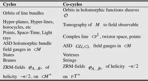
We can establish the following Table 1, using dualities.
Table 1. Some Dualities in Field Theory
Cycles Co-cycles
Orbits of line bundles Orbits in holomorphic functions sheaves
O
Hyper-planes, Hyper-lines,
horocycles, etc Tomography of M to field observable Points, Space-Time, Light
rays Complex line CP1, twistor space, points ASD holomorphic bundle
field gauges in CM ASD GL(,C), field gauges in M
C
States Vertexes Branes Strings ZRM-fields ϕA…B, of
helicity −n/2, on CM+
ZRM-fields ,
B A…
ϕ of helicity −n/2 on PT+
A duality that extends these applications to string theory and generalizes the dualities in Hecke categories context to their geometrical Langlands program is (Table 1 [17]):
M ( , Y)
G∧≅ χ ɶ
H g , (3. 3)
which was studied in [18]. Here the Lie algebra g,ɶ is the
loop extension of the loop algebra g( ).t
4. Conclusions
We want give the principles to obtain a hyper-cohomology based in extensions and generalizations of the ∂− cohomology to the space-time study, as well as give a theory of geometrical analsys and complex function theory to solve all cases of field equations as one resolution “seemed” to a Mayer-Vietoris sequence:
, ) , (
)) ( , / ( ) , ( 0
C
C →
− Π →
→ →
→
ℓ r
s D
d
H
O L G H V M
H L
(4.1)
is exact.
One possible demonstration of (4. 1) is considering the demonstration of the unitary leader representations to
), 2 , 2 (
SU through of orbits, and extended to SU(2,2)⊗G, where, is non-compact [19-21]. The orbit integrals are calculated in hyperbolic surfaces with corresponding characters to asymptotic behavior of matrix coefficients [20], of the endomorphism related with the vector bundle of Riemannian space M. The functional, of the evaluating of the twistor transform on orbits of the space SU(2,2), is a indicator of the unitary nature of the leader representations of the group SU(2,2) [6, 19]. Then the extension of the centre of the Lie algebra gC, will determine a finite number of
connected components and will can calculate the integral in
the cohomology Hs(G/L,O(L)), being =C
Q
δ
[4, 16].For other way, as has been mentioned to the equivalences (3. 3) the development that is obtained through equivalences is discovery of twistor string theory given by Witten a re-formulated by many mathematicians as Drinfeld, and other
in the geometrical Langlands program. Certain
super-symmetric scattering amplitudes with particularly neat forms in twistor space continue to be explored. The twistor methods in integral geometry admit generalizations to different space-time signatures, although all with the several versions of ∂− cohomology. This has yielded various applications in Riemannian geometry where some studies result more relevant as the study of minimal surfaces [22, 23]
References
[1] F. Bulnes, “Radon Transform, Generalizations and Penrose Transform,” Proc. 4th Appliedmath, Special Section in Functional Analysis and Differential Equations, Mexico, 2009, pp63-76.
[2] F. Bulnes, M. Shapiro, On general theory of integral operators to analysis and geometry, IM-UNAM, SEPI-IPN, Monograph in Mathematics, 1st ed., J. P. Cladwell, Ed. Mexico: 2007. [3] F. Bulnes, “Integral Theory of the Universe,” Internal. Proc.
2nd Appliedmath, IM-UNAM, SEPI-IPN, Mexico, 2006, pp73-121.
[4] F. Bulnes, “Doctoral Course of Mathematical Electrodynamics,” Internal. Proc. 2nd Appliedmath: Conferences and Advances Courses, IM-UNAM, SEPI-IPN, Mexico, 2006, pp398-447.
[5] F. Bulnes, “On the Last Progress of Cohomological Induction in the Problem of Classification of Lie Groups Representations,” Internal. Conf. of Infinite Dimensional Analysis and Topology, Book of Plenary Conferences, Precarpathian National University, Ukraine, 2009.
[6] F. Bulnes, Conferences of Lie groups (representation theory of reductive Lie groups), Monograph in Pure Mathematics, IM-UNAM, SEPI-IPN, 2nd Ed., Paul Cladwell, Mexico, 2005. [7] H. Bateman, “The Solution of Partial Differential Equations by
Means of Definite Integrals,” Proc. Lon. Math. Soc. 1 (2) (1904) 451-458.
[8] R. J. Baston, “Local Cohomology Elementary States and Evaluation Twistor,” Newsletter (Oxford Preprint) 22 8-13, 1986.
[9] R. Baston, M. Eastwood, “The Penrose Transform its Interaction with Representation Theory,” Oxford University Press, 1989.
[10] S. Helgason, The Radon transform, Prog. Math. Vol. 5, Birkhäuser, 1980.
[11] S. Gindikin, “The Penrose Transform and Complex Integral Geometry Problems,” Modern Problems of Mathematics (Moscow), Vol. 17, 1981, pp. 57-112.
[12] S. Gindikin, Between integral geometry and twistors, Twistors in Mthematics and Physics, Cmbridge University Press, 1990. [13] S. Gindikin, Generalized conformal structures, Twistors in
Mthematics and Physics, Cmbridge University Press, 1990. [14] Z. Mebkhout, Sur le problème de Hilbert–Riemann, Lecture
notes in physics 129 (1980) 99–110.
[15] M. Kashiwara, Faisceaux constructibles et systèmes holonomes d'équations aux dérivées partielles linéaires à points singuliers réguliers, Séminaire Goulaouic-Schwartz, 1979–80, exp. 19.
[16] E. Dunne, M. G. Eastwood, A twistor transform for the discrete series: the case of SU(2), Twistor Newsletter, Twistor Newsletter 26 (March 1988), pp26-30.
[17] Y. Stropovsvky, “Functors on ∞- Categories and the Yoneda Embedding,” Pure and Applied Mathematics Journal. Vol. 3, No. 2, 2014, pp. 20-25. doi: 10.11648/j.pamj.s.20140302.14 [18] F. Bulnes, Penrose Transform on Induced DG/H-Modules and
Their Moduli Stacks in the Field Theory, Advances in Pure Mathematics 3 (2) (2013) 246-253. doi: 10.4236/apm.2013.32035.
[19] I. M. Gelfand, Generalized functions, Vol. 5. Academic Press, N. Y., 1952.
[20] V. Bargmann, E. P. Wigner, “Group Theoretical Discussion of Relativistic Wave Equations,” PNAS, 34, 1948.
[21] I. Bialynicki-Birula, E. T. Newman, J. Porter, J. Winicour, B. Lukacs, Z. Perjes, A. Sebestyen, “A Note on Helicity,” J. Math. Phys., 22. 1981.
[22] F. Burstall, J. Rawnsley, Twistor theory for Riemannian symmetric space, Springer, 1990.