Bootstrap Confidence Interval for Model Based Sampling

http://www.sciencepublishinggroup.com/j/ajtas doi: 10.11648/j.ajtas.20180704.13

ISSN: 2326-8999 (Print); ISSN: 2326-9006 (Online)

Bootstrap Confidence Interval for Model Based Sampling

Thomas Mageto, John Motubwa

Department of Statistics and Actuarial Sciences, Jomo Kenyatta University of Agriculture and Technology, Nairobi, Kenya

Email address:

To cite this article:

Thomas Mageto, John Motubwa. Bootstrap Confidence Interval for Model Based Sampling. American Journal of Theoretical and Applied Statistics. Vol. 7, No. 4, 2018, pp. 147-155. doi: 10.11648/j.ajtas.20180704.13

Received: March 23, 2018; Accepted: April 15, 2018; Published: May 18, 2018

Abstract:

The bootstrap approach to statistical inference in sample surveys is an area which has seen considerable development in the recent past. In model based approach to sample survey theory the main interest has been to overcome the problem of robustness under misspecifications. The bootstrap method under restrictive model specifications has been suggested by some authors as a way of achieving this. In this study, bootstrap and conventional confidence intervals for the population total in model based surveys using the simple random sampling without replacement are constructed. This is to provide a better measure of uncertainty associated with estimates of population total as compared to the corresponding rival confidence intervals under restrictive model. In order to achieve this, generated bootstrap simulations for the population of interest in assumed general model are used. The bootstrap method is less cumbersome to apply and in terms of coverage performance in 95% confidence interval, the bootstrap method is better compared to corresponding one under conventional methods. In terms of length, the confidences generated by the bootstrap method are much smaller as compared to the conventional counterparts. It is noted that the best performing confidence interval is one whose coverage rate is close to the true population total and its length small. The study research results provides great insight in constructing better confidence interval for the finite population total estimators.

Keywords:

Bootstrap, Model Based, Confidence Interval, Sample Surveys

1. Introduction

Sample survey theory is concerned with methods of sampling from finite population of N identifiable units and then making inferences about finite population quantities on the basis of sample data. A method of sampling together with a method of estimation given the sample data is commonly known as sampling strategy which is set of rules that define how to obtain sample units from the finite population and later how to manipulate the resulting sample data to estimate the value of the population quantity. There are different approaches to specifying sampling strategy and these include, design based, model assisted and model based approaches. In considering all these approaches [1] has suggested that the model-based approach performs better than the other two approaches although no one single approach gives both efficiency and robustness.

1.1. Statement of the Problem

The major concern in model based approach to statistical

survey inference is finding robust estimators for the population parameters of interest under model misspecifications so as to make robust inference in finite populations. The authors [2] used restrictive super population model to construct confidence interval for the population mean for the case of the ratio estimator. In this study, a more general super population model to construct bootstrap confidence interval for the population total under simple random sampling without replacement is considered.

1.2. Significance of the Study

The use of general super population model, Yi =m (xi) + ei,

(i =1, 2,…, N), give rise to confidence interval of population total which is robust since all the population values Yi, (i =1,

1.3. Objectives of the Study

1.3.1. General Objective

Construct bootstrap confidence intervals for finite population total under general super population model in simple random sampling without replacement.

1.3.2. Specific Objectives

(i) Construct confidence intervals for the population total based on simple random sampling without replacement.

(ii) Simulate and determine the confidence intervals for finite population estimators using bootstrap and conventional methods.

(iii) Compare the confidence intervals for bootstrap and conventional methods.

1.4. Study Hypothesis

The 95% confidence interval for bootstrap method is better compared to corresponding conventional method.

1.5. Basic Assumptions

Given finite population P of size N, let Y denote variable of interest having values Yi, (i =1, 2… N), and X denote

auxiliary variable with corresponding population values Xi (i

=1, 2… N). It is assumed that Xi values are all known but the

characteristic values Yiare known for only the sample of n ≤

N of the population elements. A way of characterizing the sample selection of the survey variable of interest is to assume that for every unit i on the list of N units making the finite population, also known as the frame, a new variable si

takes a value equivalent to the number of times that particular population unit’s Y value is observed. The distribution of these si values defines the design of the sample survey. Once

the sample has been chosen, the values {Yj, jϵ s} are known.

The problem is how to use the sample values together with the known values of X to make an inference about unknown

population total T =

∑

=

N

1 i

i

Y . Discussion of the three

approaches of dealing with this problem, that is, the design-based approach, model assisted approach and the model based approach are presented.

2. Literature Review

2.1. Introduction

The model based approach to statistical survey has been described in [3] and [4]. The idea of non-parametric regression smoothing has been discussed in [5] and [6]. The use of non-parametric regression in estimating population parameters under conditions of missing data has been discussed in [7]. The author [8] considered a non-parametric regression model estimating population totals in finite populations. In the study, non-parametric regression based estimators for the population total and compared performance corresponding to design based and linear

regression estimators were considered.

The authors [9] assumed non-parametric regression model and developed new class of model assisted estimators for T based on local polynomial regression. In the simulation study, their estimate performs better than the Horvitz-Thompson estimator. In sample survey theory, it is important to construct confidence interval for the population parameter under investigation. One way of achieving this is through the conventional method. As noted earlier, the conventional method assumes that the sample size is large enough for the central limit theorem to be applicable. However, this is not always true, as consequence of this, [2] proposed the bootstrap methodology as way of addressing this problem.

The bootstrap approach to statistical inference is described in [10] and in the study it has been demonstrated how to apply the bootstrap in design based survey sampling under different sampling designs including stratified cluster sampling with replacement, stratified simple random sampling without replacement, unequal probability sampling without replacement and two stage cluster sampling with equal probabilities and without replacement. The use of the bootstrap in model-based surveys was first suggested by [11] and developed by [2]. The latter work forms the basis of this research work. The method of constructing confidence intervals as suggested by [2] involved the use of the mean and the variance. The authors made use of linear unbiased estimator obtained from the ratio between the mean of the y-sample and the x-y-sample together with the ratio estimator. The model based approach to the above problem is based on the assumption that the values of Y can be assumed to be realizations of random variables whose distribution conditional on the known values of X may be specified through a convenient probability model, [2] proposed modifications of their procedure to take account of misspecifications in the working model. They noted that there was greater efficiency in the use of successive model refinements estimators obtained using the bootstrap approach as opposed to rival estimators obtained by other methods. However, the evidence of the extended simulation study showed that the achievement of their research did not precisely attain its goal. The recommended construction of confidence interval using the bootstrap approach thus requires further investigation.

2.2. Design-Based Inference

randomization. In probability sampling designs, it is assumed that each Y_i (i=1, 2, ..., N) in the population has definite probability of being included in the sample. This approach however requires infinite sequence of sample values so as to apply the central limit theorem, consequently, it is best suited for large scale surveys.

The main concept under this approach in solving the above problem is that of design unbiasedness, that is, for any choice of sampling process S, the weighted average value of Tˆ over all possible samples generated under S is the actual value of T. Thus this approach restricts consideration to those weights W which ensure that irrespective of the sample selection chosen (that is, S),

ˆ

E(T T|X,Y)

−

= 0, for all values of X and Y.

However, as noted by [1] no uniform optimal sampling strategy exists under the design based approach, for example, consider the population defined by Yi > 0 and Yj > 0, i ≠ 1

and use the weighting scheme W1-1 = E (S1|X), then;

ˆ

Var(T T|X,Y)

−

=0

If the is chosen so that,P(S₁−1|X−1), such that E (S1|X) =

1. However, this restricted strategy is no longer optimal if we apply it to another population where Yi > 2 and Yj = 0, j ≠ 2.

2.3. Model Based Inference

The model based approach to statistical survey sampling has been described and developed in [3] and [4]. The idea of non-parametric regression goes back to [5] and [6]. The model based approach to the above problem is based on the assumption that the values of Y can be assumed to be realization of random variables whose distribution conditional on the known values of X may be specified through a convenient probability model. For example, consider a linear regression model in which;

i

Y =α+βxi+σ(x )ei i i =1, 2, …, N (1)

Where α and β are unknown, σ(x_i)is known and {ei} is a

sequence of independently and identically distributed random variables with zero and unknown variance.

In estimating the population total T, consider the relation;

T= _i

s

y

∑

+ _j

r

y

∑

(2)

Where

∑

s i

y and

∑

r j

y denote summations over sample

and non-sample values respectively. Hence the problem of estimating T is the problem of predicting sum of unobserved random variables

∑

r j

y . The sample is used to infer about the

model and also used to predict, j r

y

∑

. Thus the estimate of the population total T is the minimum variance unbiased linear estimator.

lin

T = i j

i s j r

ˆ ˆ y (α βx )

∈ ∈

+ +

∑

∑

(3)

Where ˆα and ˆβ are the best predictors of α and β respectively.

The problem in the model-based approach to survey sample is finding robust estimators for the population parameters of interest. Suppose the population value Y is assumed to be generated by the following linear regression model;

i i i

E(Y |X =x ) =βxi

i i i

Var(Y |X =x ) =

σ (x )

2 i

i j i i j j

Cov(Y , Y |X =x , X =x ) =0, i≠ j (4)

Where β and σ2(x_i) are unknown positive constants. The

best linear unbiased estimator of β is βˆ=

s s

x y

while the best

linear unbiased predictor of T is the ratio estimator TˆR =

X βˆ

N where y_s and x_s are the means of the sample values of Y and X respectively and Xis the population mean of X. It is noted that model (4) states that the regression line of Y on X passes through the origin and that Yi, are independent.

Suppose some of these conditions or all are not true, will the ratio estimator still be unbiased? Will it still be optimal? Such problems are known as robustness problems. Thus robustness problems are those that point out the weaknesses of the estimator under application. An estimator which is optimal under the assumed model and remains optimal or approximately so when there are errors in the model is considered and is commonly referred to as robust estimator.

The non-parametric regression model for estimating population totals in finite populations was considered by [8]. The non-parametric regression based estimator for population total was proposed and in developing estimator, it was assumed that population values are generated by model given by;

Yi =m(xi)+ei, i =1, 2, …, N (5)

Where m (·) is a smooth function, {ei} is a sequence of

independent random variables with mean zero and variance, )

σ(x_i , (i =1, 2, ..., N )

The non-parametric population total estimator due to [8] is given by;

TD = i j

s r

Y+ m(x )

∑

∑

(6)

Where m(xj) = i j i

i s

w (x )y

∈

∑

and w_i =

i j i j i s

x x x x

k k

h _∈ h

− −

   

÷

   

ith unit of sample for selected bandwidth h. The error variance of (6) is given by Var(T_D−T|X )_p =

2 2 2 i i i s s

w σ (x )+ σ (x )

∑

∑

due to [8]. In the empirical study,

[8] illustrates that the estimate TˆD performs well compared to the corresponding design based and linear regression estimators. Author [7] also discussed the use of non-parametric regression estimating population parameters under conditions of missing data. However, the work by [8] has yet to be extended to more complex designs such as two stage cluster sampling.

2.4. Model Assisted Inference

Consider a general linear estimator of T of the form;

Tˆ =

∑

=

n

1 i

i i(S,X)S Y

W (7)

In this model W (S, X) is the weight of the sample _i associated with population unit j when unit is selected into the sample. Hence the sampling strategy consists of;

(i) Given X, choosing an appropriate distribution of S. (ii) Given S and the distribution generated under (i),

choosing an appropriate specification for W.

In order to estimate T, the model assisted approach assumes that the resulting estimator Tˆ is design unbiased, or approximately. The distribution for S is sought which minimizes the expected value of the design mean squared error;

ˆ

MSE(T|X,Y)

=

Var(T|X,Y) E (T-T|X,Y)

ˆ

+

2

ˆ

If Y values are consistent with the known values in X. The author [1] argues that there are many other design unbiased strategies which also satisfy the average design unbiasedness condition;

ˆ

E(T-T|X)

=

E(E(T-T|X, Y)|X)

ˆ

=0

However this condition is weak, [9] assumed model (6) and developed new of model-assisted estimators for T based on local polynomial regression. The estimator is given by;

LP

Tˆ =

∑

∑

∈ ∈ +         ₋ u i i s i i i i _m π m y

, i =1, 2, …, N

Where πi = P(i∈s) , mi = w_s−1y_s , wsi =

            − i π 1 h xj xi k h 1

diag ,j∈s

In simulation study, TLP performs better than the

Horvitz-Thompson estimator

HT

ˆ

T

= i

i i s y π ∈

∑

The work by [9] was recently extended to two stage sampling by [13] and [1] has considered a uniformed framework for survey design and estimation, that is, design-based approach, the design-based approach and the model-assisted approach. In contrasting them on the basis of their concepts of efficiency and robustness based on the assumptions about the characteristics of the finite population, it is concluded that, although no any of these approaches gives both efficiency and robustness, the model based approach performs better than design and model assisted approaches. The authors [2] have proposed the bootstrap to overcome the above problem and assumed a restrictive non-parametric model to construct bootstrap confidence interval even when the sample is not large for the central limit theorem to hold. In order to obtain robust confidence interval they subjected their model to multiple modifications. The empirical results showed that their objective which was to construct a sound confidence interval was not attained. In this study, the application of bootstrap method to construct a confidence interval for the population total T assuming a general supper-population model as a working model is considered. This consideration will lead to avoiding multiple modifications undertaken by [2].

3. Methodology

3.1. Sample Size

The sample size for the finite population is obtained using [14] formula given by

n = P) P(1 X 1) (N d P) NP(1 χ 2 2 2 α 1 − + − −

− ₍₈₎

Where n –sample size, N – Population size, d – The degree of accuracy expressed as proportion, P – Population

proportion, χ2_1−α – tabulated value of chi-square for 1 degree of freedom at desired confidence level.

3.2. Selection of Bandwidth for Gaussian Kernels

The optimal bandwidth is selected based on results from various techniques [15] that include considering common variation using factor 1.06 denoted (nrd), rule-of-thumb for choosing bandwidth of Gaussian kernel density estimator (nrd0), implementing unbiased cross-validation (ucv), implementing biased cross-validation (bcv) and determination of bandwidth that minimizes estimation (mcv)

of finite population total error

2 n -N r i i n s i i i

j(x )y y

w _

      −

∑

∑

∈ ∈ .

3.3. Confidence Intervals

population total T. The conventional method to achieving this is to calculate the model unbiased point estimator V of the model variance of the estimation error, Tˆ-T. Researchers have suggested some model variance estimators, for instance the heteroscedasticity robust estimator investigated by [16] and [17] for the population mean Yof the ratio estimator YR.

This is given by;

p V = 1 2 s s 2 D n C 1 X X NX N n 1 n σ −         −       −

Where σ_D2 =

∑

∈

− − _{i s}

2 i i βˆx ) (y 1 n

1

, C_s2 =

∑

∈ − − s j 2 s j X )

(X X 1) n

1

, X

and Xs denote the population mean of X and sample

respectively. The authors [11] have considered application of the bootstrap to estimate the model variance. There estimator under general conditions is given as;

MB

V = _

       + −

∑

∑

∉

i i s i i 2 i

2 _{(w 1) Ω Ω}

σ

Where wi correspond to the ridge weight I and

Ω

is an

N*N diagonal matrix of known constants, Ω_i, i =1, 2, …, N independent of Y,

2 σ =

∑

∑

∈ ∈ − − s i i i s i 2 i i 1)Ω (w 1)ε (w

, ε_i = Y_i−XT_iβ , β =

Y W X X) W X U UC

(λ −1 + T −1 −1 T −1 , C is a diagonal matrix, λ

is a ridge parameter and U =diag (u1, u2, …, ub). Using

conventional method, 100 (1-α) % confidence interval for the population total T [18] and [19] is given by;

1) n α/2, t(1 V

T± 1/2 − −

Where t(1−α/2, n-1) is the (1−α/2) quartile of the t-distribution with n-1 degree of freedom, of the estimation error Tˆ-T. However, the conventional method is based on the assumption that the sample size is large enough for the central limit theorem to apply but this is not always true in practice.

3.4. Bootstrap Confidence Intervals

The model assumed is;

i

Y =m(xi)+σ(xi)ei i=1, 2, ..., N (9)

Where m ( ) is a smooth function, e_i is an independent random variable with mean zero constant variance, σ(⋅) is a smooth and non-negative function. The bootstrap simulations for the population Y by use of the model are generated;

D

Tˆ =

∑

∑

∈ ∈ + r j j s i

i mˆ(x )

Y (10)

Where mˆ(x_j) =

∑

∈s i

i j i(x )y

w , w_i(x_j) is the weight

associated with the ith unit of the sample.

This is the mean function with bandwidth h. In this study, the expected value and variance of the residuals R_i =

) m(x

Y_i− _i , i=1,2,..., n are obtained. This will help in obtaining a properly scaled residue to estimate e_i in model (2). Let this scaled residual be R*_i, i=1,2,..., n and obtain a bootstrap simulation of the population values sampled

without replacement for R*_i, i=1,2,..., n and calculate Yj* = *

j i i) σ(x )R

m(x + , (i, j∈s), i≠j. This is done N times to obtain

bootstrap valuesY₁* ,Y₂*, ...,Y_N* . Then TD given in (10) is

calculated to obtainTD*i. The above procedure is repeated a large number, B, of times to obtain TD*1, TD*2, ..., TD*B. Lastly the lower and upper percentiles are calculated [20].

3.5. Conventional Confidence Intervals

In obtaining conventional confidence interval, the model unbiased point estimate of the variance σ(x_j) (j=1,2,...,n) is calculated as given by [8] such that;

1 , 1) n α/2, )t(1 (x σˆ

Tˆ± 2 _j − − α< (11)

Where

) (x σ2 _j

=m (x )-m (xj)

2 h j

21 ₍₁₂₎

) (x m_{21 j} =

∑

∑

∈ ∈       −       − s i s i 2 i h xj xi k y h xj xi k (13) ) (x mh j =

∑

∑

∈ ∈       −       − s i s i i h xj xi k y h xj xi k (14)

Where h is the bandwidth and mh(xj) is a pilot estimator

based on the scaling factor h. It is noted that the estimator (12) can be negative, the suggestion by [8] is adopted in which the negative values are ignored since negative values offer no significance in the study.

4. Statistical Analysis

4.1. Introduction

values while 1930 values are taken to be the Y values. The regression of Y on X is approximately linear and hence the population total for any state in 1930 largely depends on corresponding size in 1920 as shown in Table 1 based on parametric linear regression test [22] on testing hypothesis H0: β1 =0 against Ha: β1 ≠ 0 at α =0.05 level of significance.

The test statistic t =35.383 equivalent to p-value less than 0 is an indication of linear regression such that β1 ≠ 0 at α =0.05

level of significance.

Table 1. Linear regression analysis of variance.

Coefficients Estimated Std. Error t-value p-value

β0 8.38396 4.77716 1.755 0.0858

β1 1.15773 0.03272 35.383 0.0000

In each sample randomly selected from the population, both the bootstrap confidence interval and the conventional confidence intervals are calculated and the results given in tabulated form. Later, the coverage rates for the two methods are obtained to compare the performance.

4.2. Procedure

The survey variable of interest is Yi (i =1, 2, …, 49) is

considered and that these values are known only for the sample while the auxiliary variable Xi (i =1, 2, …, 49) in the

population are known. Independent 1000 samples of size 44 from population are drawn by simple random sampling without replacement using sample size determination relationship considered in [14]. Now considering sample values of Y selected from the population and the corresponding known values of X the non-sample values are estimated so as to obtain TD. In achieving this, the following

assumptions are made:

(i) K (u) is a standard normal density function and since this function is symmetric, it meets the required criterion.

(ii) An optimal bandwidth would be to select h such that it minimizes the mean average squared error TD – T,

where TD is given in equation (10).

In obtaining bootstrap simulation for the population values, samples without replacement are selected, further, using the above assumptions, the bootstrap value for Yi is

calculated denoted as Yi* =m(xi)+Ri*, (i, j∈s, i≠j). Then TD in (10) is calculated to obtain T*D. This is repeated 1, 000

times to obtain, T∗ _{, T}∗ _{, …, T}∗ _{for samples.}

In order to obtain the 95% bootstrap confidence interval for population total, the data is arranged in order of size from the least to the largest then the 2.5 percentile and the 97.5 percentile bootstrap population values for population total for samples are determined. This is repeated for 1,000 iterations to obtain 1,000 lower and upper confidence interval for the population total T. In evaluating the corresponding conventional confidence interval for the same sample the model unbiased point estimate σ (xi) for the population total

given by (12) is considered and lower and upper conventional confidence limits are calculated using the formula;

1) n α/2, t(1 N ) (x σˆ

Tˆ± _i − −

The above procedure is repeated for 1,000 iterations for subsequent samples drawn from population without replacement. Further, number of times each method covered true population total, T = 6, 262 are counted in order to obtain the coverage rates under considered methods. That is,

Coverage rate =

100 s iteration of Number

total population true

the contains interval the times of Number

×

4.3. Empirical Results

The methods of estimating the finite population are compared using the mean square criterion given asMSE =

∑

= −

1000

1 i

2

T) Tˆ ( 1000

1

for twenty sample groups, that is, for each

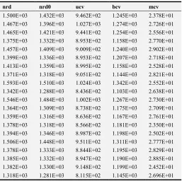
technique determine the mean square for the 1st 1000 samples, 2nd 1000 samples till the 20th 1000 samples group and results recorded in Table 2. It is observed that minimizing cross validation (mcv) procedure has least mean square error followed by unbiased cross validation (ucv) and biased cross validation procedures while rule of thumb (nrd0) using factor 1.34 and rule of thumb using factor 1.06 have higher mean square error. The procedures with less mean square error are considered better compared to the ones with higher mean square values in estimating finite population total.

Table 2. Mean square error of various finite population total estimating methods.

nrd nrd0 ucv bcv mcv

1.500E+03 1.432E+03 9.462E+02 1.245E+03 2.378E+01

1.467E+03 1.396E+03 1.027E+03 1.274E+03 2.726E+01

1.465E+03 1.421E+03 9.441E+02 1.254E+03 2.556E+01

1.375E+03 1.332E+03 8.953E+02 1.158E+03 2.770E+01

1.457E+03 1.409E+03 9.009E+02 1.240E+03 2.902E+01

1.399E+03 1.336E+03 8.953E+02 1.207E+03 2.718E+01

1.413E+03 1.359E+03 8.995E+02 1.158E+03 2.528E+01

1.371E+03 1.318E+03 9.051E+02 1.144E+03 2.821E+01

1.593E+03 1.510E+03 1.024E+03 1.342E+03 2.552E+01

1.342E+03 1.288E+03 8.436E+02 1.103E+03 2.638E+01

1.546E+03 1.484E+03 1.002E+03 1.267E+03 2.730E+01

1.364E+03 1.309E+03 8.738E+02 1.175E+03 2.709E+01

1.359E+03 1.316E+03 8.636E+02 1.167E+03 2.761E+01

1.378E+03 1.318E+03 8.566E+02 1.181E+03 2.350E+01

1.394E+03 1.346E+03 8.987E+02 1.198E+03 2.502E+01

1.506E+03 1.448E+03 9.511E+02 1.311E+03 2.777E+01

1.378E+03 1.333E+03 8.844E+02 1.195E+03 2.829E+01

1.385E+03 1.332E+03 8.947E+02 1.190E+03 2.885E+01

1.382E+03 1.330E+03 9.148E+02 1.199E+03 2.452E+01

1.318E+03 1.281E+03 8.115E+02 1.145E+03 2.696E+01

Figure 1. Chart of mean square error for finite population total estimating methods.

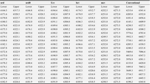
The results of corresponding confidence intervals for the population totals are presented in Table 3. In terms of coverage performance the 95% confidence interval, results of

conventional method indicates that it has higher coverage compared to family of nonparametric methods as shown in Figure 2.

Table 3. Confidence intervals for family of nonparametric and conventional methods.

nrd nrd0 Ucv bcv mcv Conventional

Lower Upper Lower Upper Lower Upper Lower Upper Lower Upper Lower Upper

6164.3 6317.3 6166.8 6316.1 6184.4 6302.1 6174.3 6312.7 6252.5 6271.5 6215.6 6341.4

6171.6 6320.5 6173.6 6320.5 6182.4 6307.9 6178.9 6317.7 6251.0 6272.0 6205.0 6352.0

6170.8 6323.7 6171.0 6322.6 6188.4 6303.6 6176.2 6318.5 6252.0 6272.0 6101.4 6456.6

6180.3 6322.6 6182.0 6323.9 6191.1 6304.0 6186.3 6319.2 6251.0 6272.0 6145.1 6409.9

6176.0 6321.8 6176.9 6322.5 6189.4 6303.1 6180.2 6314.6 6252.0 6273.5 6230.5 6327.5

6175.3 6322.1 6176.1 6323.9 6190.0 6305.2 6183.9 6313.9 6252.0 6272.0 6260.8 6300.2

6175.0 6320.1 6175.0 6322.0 6188.2 6301.9 6182.2 6315.6 6252.0 6271.5 5774.6 6783.4

6179.1 6323.1 6180.2 6323.4 6191.5 6306.0 6185.8 6316.1 6249.5 6272.0 5952.3 6602.7

6168.6 6324.3 6170.4 6318.6 6185.8 6306.8 6178.8 6317.2 6252.0 6272.5 5710.1 6851.0

6182.1 6325.0 6182.9 6322.9 6190.2 6303.2 6186.6 6317.1 6252.0 6272.0 6205.5 6350.5

6167.8 6324.8 6170.7 6323.0 6180.4 6304.4 6178.8 6313.5 6252.0 6272.0 6240.2 6321.8

6172.4 6322.9 6175.0 6322.9 6189.8 6307.9 6178.8 6317.2 6251.0 6272.0 5469.6 7086.4

6175.0 6319.1 6175.6 6319.3 6190.9 6305.7 6179.1 6316.2 6250.5 6272.0 6013.8 6547.3

6177.9 6321.4 6179.7 6319.5 6192.0 6304.0 6178.6 6317.2 6252.0 6272.0 5976.9 6581.1

6178.2 6322.8 6180.4 6322.2 6189.8 6305.4 6184.2 6318.5 6251.5 6272.0 6133.0 6428.0

6174.1 6323.0 6173.0 6321.2 6187.7 6305.6 6174.2 6314.9 6251.0 6273.0 5495.8 7065.2

6175.2 6322.5 6178.6 6321.3 6190.0 6305.1 6182.3 6320.6 6252.0 6273.0 5649.3 6911.7

6177.0 6323.6 6177.9 6325.1 6188.8 6304.9 6182.1 6318.9 6251.5 6273.0 5718.5 6837.5

6174.4 6322.3 6172.4 6321.4 6188.1 6306.2 6177.1 6316.4 6252.0 6272.0 6109.7 6445.3

6182.5 6324.4 6181.9 6325.6 6191.9 6303.9 6185.0 6318.5 6250.5 6271.5 6190.2 6365.8

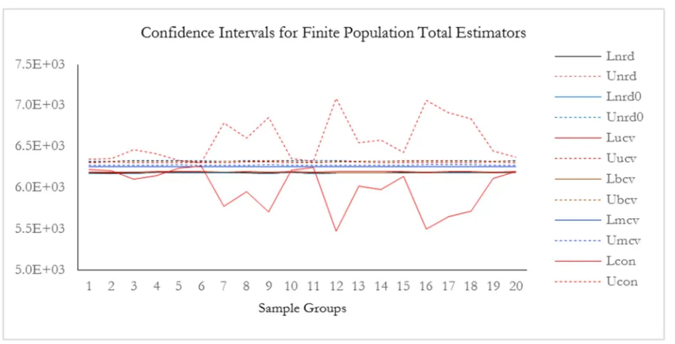
In terms of length, confidences generated by family of nonparametric methods are much smaller compared to conventional counterpart. It is noted that best performing confidence interval is one whose coverage rate is close to

cross validation and biased cross validation techniques perform better compared to rest of bootstrap confidence

interval methods as shown in Figure 2.

Figure 2. Confidence intervals for finite population total estimators.

5. Conclusions and Recommendations

5.1. Conclusion

The main objective of the study is constructing confidence intervals for the population total based on simple random sampling without replacement. The investigation focused on application of a general super population model. The evidence of the extended simulation study has shown that there is greater coverage rate using the bootstrap method as opposed to the conventional method, thus, the result is consistent with research objective. The results of this study could be used in any statistical data containing bivariate data X and Y, where values Y1, Y2, …, YN are independent

whereas values for auxiliary variables X1, X2, …, XN are well

known and those for the survey variable Y are known only for the sample.

5.2. Recommendations

(i) This study is computer intensive where simulations of the population values using 1,000 samples in simple random sampling without replacement was considered. There is need to extend study to larger or very large sample simulations given appropriate application package or computer program.

(ii) The study work could be extended to two stage sampling and model assisted approach.

(iii) Further research on the comparison of these research results with the one under a restrictive model can be considered as part of extension on this study.

References

[1] Chambers, R. L. (2011). Which Sample Strategy? A Review of Three Different Approaches, Centre for Statistical and Survey Methodology. University of Wollongong, Working Paper 09-11, 2011.

[2] Chambers, R. L., and Dorfman, A. H. (2003). Robust Sample Survey Inference via Bootstrapping and Bias Correction: The

Case of the Ratio Estimator. Southampton: Southampton

Statistical Sciences Research Institute 21pp. (S3RI Methodology Working papers, M03/13).

[3] Smith, T. M. (1976). The Foundations of Survey Sampling: A Review. Journal of the Royal Statistical Society, A 139, 183-204. [4] Smith, T. M. (1984). Sample Surveys: Present Position and

Potential Development: Some Personal Views. Journal of the Royal Statistical Society, A 147, 208-221.

[5] Nadaraya, E. (1964). On Estimating Regression. Theory Probability and Applications, 9 141-142.

[6] Watson, G. S. (1964). Smooth Regression Analysis. Sankhya, A 359-372.

[7] Cheng, P. E. (1994). Non-parametric Estimation of Mean Function with Data Missing at Random. Journal of the American Statistical Association, 89, 81-87.

[8] Dorfman, A. H. (1992). Nonparametric Regression for Estimating Totals in Finite Populations. Proceedings of the Section on Survey Research Methods. American Statistical Association, 88, 622-625.

[9] Opsomer, D. J., & Breidt, F. J. (2000). The Application of Local Polynomial Regression to Survey Sampling Estimation.

[10] Rao, J. N., & Wu, C. F. (1988). Resampling Inference with Complex Survey Data. Journal of American Statistical Association, 83, 231-241.

[11] Do, K. A., & Kokie, P. (2001). Bootstrap Variance and Confidence Interval Estimation for Model-Based Surveys.

Technical Report, ustralia National University.

[12] Godambe, V. P. (1955). A Unified Theory of Sampling from Finite Populations. Journal of the Royal Statistical Society, Series B (Methodological), Vol. 17. No. 2 pp. 269-278. [13] Kim, T. H., & Christopher, M. (2003). Two Stage Quartile

Regression when the First Stage is Based on Quartile Regression. Journal Statistical Association, 7, 218-231. [14] Mageto, T., & Zablon, A. (2018). Modeling Self Medication

Risk Factors (A Case Study of Kiambu County, Kenya).

American Journal of Theoretical and Applied Statistics, 7(2), 58-66.

[15] Venables, W. N., & Ripley, B. D. (2002). Modern Applied Statistics with S. Springer.

[16] Royall, M. R., & Cumberland, G. W. (2012). Variance Estimation in Finite Population Sampling. Journal of the American Statistical Association, 73:362, 351-358.

[17] Royall, R. M., & Cumberland, W. G. (1981a). An Empirical Study of the Ratio Estimator and Estimators of its Variance.

Journal of the American Statistical Association, 76, 66-77. [18] Helwig, E. N. (2017). Bootstrap Confidence Intervals.

Minneapolis and Saint Paul: University of Minnesota (Twin Cities).

[19] Puth, M.-T., Neuhauser, M., & Ruxton, D. G. (2015). On the Variety of Methods for Calculating Confidence Intervals by Bootstrapping. Journal of Animal Ecology, 84, 892-897. [20] Fox, J., & Sanford, W. (2017). Bootstrapping Regression

Models in R. An Appendix to An R Companion to Applied Regression, pp. 1-20.

[21] Cochran, G. W. (1992). Sampling Techniques. New Delhi: Wiley Eastern Limited.