Identification of Structural Parameters Using Combined Power Flow
and Acceleration Approach in a Substructure
Cibu K. Varghese
1, K. Shankar
2,*Machine Design Section, Department of Mechanical Engineering, IIT Madras, Chennai, India.
Received 23 July 2011; received in revised form 21 August 2011; accepted 27 September 2011
Abstract
This paper presents the application of a power flow parameter to improve system identification results when used along with conventional acceleration matching techniques. In this paper the power balance concept is implemented in a substructure to estimate the stiffness and damping coefficients from time domain responses. Power flows are calculated using the time averaged product of force and velocity at the input and substructure interfaces of a substructure. The concept of power flow balance through the substructures is to equate the input power against the dissipated and transmitted powers and by reducing any imbalance to zero using optimization methods. No extra sensors are needed to include criteria of power flow balance along with acceleration matching. Numerical simulations are performed for substructures from a 10 degree-of-freedom (DOF) lumped mass system, a planar truss of 55 elements with 44 DOF and a cantilever beam of 20 elements to evaluate the feasibility of the proposed method. In numerical simulations, noise free and noise contaminated response measurements are considered. The Particle Swarm approach is used as the Optimization algorithm, and the fitness function is defined to minimize the error with weighted aggregation multi-objective optimization (MO) technique. The results demonstrate that the proposed combined method is more accurate in identifying the structural parameters of a system compared to conventional acceleration based matching methods.
Keywords: power flow, substructure, system identification, structural response, time domain
1.
Introduction
Structural parameters can be identified with the inverse analysis of input and output of the structural system. The term inverse problem is used to denote a class of problems in which it is required to construct a system from specified system behavior. Input and output data of dynamically excited structures are measured and numerically processed to identify the structural parameters. System identification from measured input/output data has gained great importance due to the availability of powerful identification algorithms. Study of power flow balance in practical structures subjected to various excitations can improve structural identification when combined with conventional acceleration matching method.
Lyon and Maidanik [1] calculated power flows between two independently and randomly excited harmonic oscillators assuming small linear coupling and using power flow model computed steady state partition of energy between the two systems and the parameters which govern the partition. Bishop and Johnson [2] proposed the method of receptances to predict
*Corresponding author. E-mail address: [email protected]
the vibrations of a combined system from the subsystem receptances, an approach that is extensively used in frequency domain power flow calculations. Shankar and Keane presented a model of complex cantilever structure for evaluating the energy flows at the free end when excited near the base based on receptance theory [3]. The receptance method has the ability to directly calculate substructure energy transfers, as it deals with the junction forces and displacements.
A finite element analysis model was presented in [4], for substructuring using free-free interface conditions to evaluate eigenvalues and eigenvectors. In the above work the time averaged substructure vibrational energy levels are calculated by balancing the input and dissipated energies along with the energy transferred through the coupling nodes. Wang et al. [5] determined power flow between the interfaces of substructures using free-free interface conditions deducing displacement contribution of the external and boundary coupling forces. The method formulated is used in the power flow analysis of a simple rod truss system and in a more complex system. Time averaged vibrational power input to a structure is defined as the product of harmonic excitation and resultant velocity at the driving point [6].The concept of power flows through the structure was used to determine the time averaged energy levels of each member in the structure fitted with tuned vibration absorbers [7]. The method used in the aforementioned study calculates power flows using the time averaged product of force and velocity at the input and coupling points of a general structure made of axially vibrating rods. Fahy pointed out some of the advantages of studying power flows as, various components of power flow can be summed up and power flows between various members obey the law of conservation of energy [8].
Koh et al. [9] decomposed structures into subsystems using the method of extended Kalman filter with a weighted global iteration algorithm, to solve the state and observation equations for improved convergence and efficient computation of structural parameters. A non classical approach of genetic algorithms (GA) as a search tool to identify unknown structural parameters was employed with substructural and progressive identification methods [10]. Substructuring will reduce the number of unknown structural parameters to be identified, so that the identification effort and difficulty can be reduced. The requirement of interface measurement, which is difficult to get in certain cases like beam or frame rotational response are eliminated on the basis of receptance theory, which requires different sets of measurements in the substructure under dynamic excitation [11]. Sandesh and Shankar identified simultaneously the structural parameters and input time history of the applied excitation based on substructural approach [12]. The unknown interface forces at the end of the substructure are also identified iteratively using the substructure method. The substructure based structural analysis techniques show that the convergence conditions of the identification procedure are improved significantly along with reduction in computational time.
In the present study, MO (Multi-objective Optimization) of combined power flow balance and conventional acceleration matching has been used for the identification of structural parameters in the time domain. It may be noted that power flow parameter can be also introduced in the frequency domain knowing the input and interface receptances. A search of literature shows that this concept of power flow balance for structural identification has not been investigated yet and the authors believe it is a novel contribution. In this paper, the proposed method is applied on various types of substructures, and the improvement in accuracy shown. The heuristic Particle Swarm algorithm has been used for optimization because of its ability to attain the global minima in a search space dominated by many local solutions.
2.
Substructure Method
identification because of numerical difficulty in convergence. It is therefore makes sense to divide the structure into smaller substructures, for which DOFs will be small, require fewer sensor measurements and no need to know responses outside substructure. The equation of motion for a complete linear structure comprising of spring mass damper system can be written as
( ) ( ) ( ) ( )
Mx t +Cx t +Kx t =P t (1)
Where M, C and K are the mass, damping and stiffness matrices, respectively x is the displacement vector, the over dot denotes differentiation with respect to time t and P(t) is the excitation force vector. The equation of motion (2) for complete structural system can be written as explained by the method described in [10] and [13].
u u u f u u u u f u u u u f
f u f f f r f f u f f f r f f u f f f r
r f r r r g r f r r r g r r f r r r g
g r g g g d g g r g g g d g
d g d d d d g d d d
M M C C K K
M M M C C C K K K
M M M C C C K K K
M M M C C C K
M M C C
r x x x x x x x x x x + + u u f f r
g r g g g d g g
d g d d d d P
P
P
K K P
K K P
r x x x x x = (2)
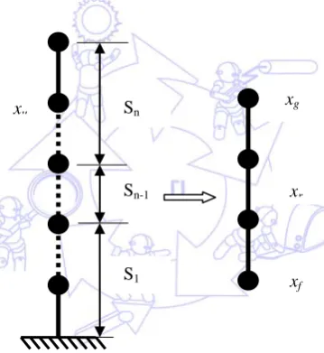
Where the subscript r denotes internal DOFs of the concerned substructure, subscripts f and g represents the interface DOFs, u and d represents the DOFs of the remaining structure on either side, as shown in Fig. 1.
Fig. 1 Multiple DOF system and substructure
In dynamic structural analysis damping plays an important role, among the various damping models, the modal damping and Rayleigh damping models are most frequently used to model the structural damping [12]. The current formulation employs Rayleigh damping for SI. In Rayleigh damping, a damping matrix is represented by a linear combination of the mass and stiffness matrix.
C=αM+ βK (3)
Where α and β are Rayleigh damping coefficients decided from modal information of two modes. The equations of motion for the substructure considered may be extracted from the system of partitioned equations following the method described in [10].
{ ( )}
f f f
r r r g r r r g r r r rg r r
rf rf rf
g g g
r
x x x
M M M x C C C x K K K x P t
x x x
+ + = (4)
{ ( )}
j j j
rr rr r r r
rj rj rj
r r
r
x x x
M M C C K K P t
x x x
+ + =
(5)
Where subscript j represents combined DOFs f and g at interface for concise representation. Equation (5) can be rearranged to bring the interior partitions to the left and interface effects in the form of a force on to the right as,
( ) ( ) ( ) ( ) ( ) ( ) ( )
rr r rr r rr r r rj j rj j rj j
M x t +C x t +K x t =P t −M x t −C x t −K x t
(6)
Pr(t) is the force applied on the interior node(s). If there is no excitation within the substructure, Pr(t) is set to zero and in
that case force is applied outside the substructure. The left side of the (6) represents the inertia force, damping force and restoring force components acting in the substructure which is treated as output from the substructure. The right side of the (6) is treated as input to the substructure. Excluding Pr(t) term represents forces induced by motion relating to interface DOFs and
may be referred to as interface motion forces. To compute the interface motion forces (coupling forces) the substructure interface displacements, velocities and accelerations are required. These interface accelerations x double dot j has to be obtained experimentally, and thereafter integrated to obtain the velocities x dot j and displacements xj.
2
1 , ,
1 1
( )
N L
m e
ij ij i j
f x x
= = =
∑∑
−A few experimentally measured acceleration response x double dot m at N points inside the substructure are also required. The estimated accelerations x double dot e at N points are obtained from the mathematical model from the left hand side of (6). For correct identification, x double dot e has to match with the experimentally measured response x double dot m. Here experiments are numerically simulated from responses generated from a known numerical model and polluted with Gaussian noise of zero mean and a certain percentage of standard deviation for realism. Using Particle Swarm optimization algorithm the following fitness function is minimized, for single objective acceleration matching which is the first goal of the proposed method.
(7)
The superscripts m and e denote measured and estimated responses for fitness evaluation. L is the number of time steps and N is the number of measurement sensors used. Ideally it must be minimized to zero, but usually it approaches a value close to zero.
3.
Power flow Calculations
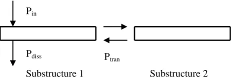
The concept of time averaged power flow is illustrated in Fig. 2, which shows the power flow between substructure1 and substructure2 when the former is excited by a force, F(t). The applied excitation introduces input power (Pin) into the
substructure1 which depends on the time averaged product of force and velocity at the forcing point of the substructure1. The output power (Pout) is made up of two components as discussed below. A portion of (Pout) is dissipated in substructure1 itself
(Pdiss) due to damping effects in that substructure, whereas the other portion (Ptra n) is transmitted across the interface to
adjacent substructures.
Fig. 2 Components of power flow in substructure 1 Substructure 1 Substructure 2
Ptran
Pin
When both substructures are excited it is possible for net power transmission across the interface to occur from substructure1 to substructure2 or vice-versa, depending on which substructure is subjected to stronger excitation and other factors. The time averaged power at any point in terms of force, F(t) and velocity, V(t) over a period, T is given by,
0
( ) ( ) TF t V t
P dt
T
=
∫
(8)The steady state time averaged power balance equation of substructure is given by,
. . 0
in out
P +P = (9)
. . . 0
in tran diss
P +P +P = (10)
The power input to the substructure can be represented as,
. 0
( ) ( ) T
r r
in
P t x t
P dt
T
=
∫
(11)Pr(t) is the applied force inside the substructure node(s) and x dot r is the respective nodal velocity inside the substructure
where the applied force acts. The substructure interior velocity x dot r is not explicitly measured at any sensor. It is calculated by the optimization algorithm by trying various values of x dot r. At the right value of stiffness and damping coefficients correct values of x dot r
Power transmitted across the substructure interface can be represented as, are obtained.
. 0
[ ( ) ( ) ( )] ( )
T rj j j j r
tran
rj rj
M x t C x t K x t x t
P dt
T
+
+
=
∫
(12)The term inside the square bracket represents interface motion forces (coupling force) acting at the substructure interface and is evaluated as explained in (6). The interface accelerations x double dot j has to be obtained experimentally, and thereafter integrated to obtain the velocities x dot j and displacements xj
The power dissipated in the substructure due to damping is given by
to evaluate power transmitted.
. 0
[ ( )] ( ) T
rr r r
diss
C x t x t
P dt
T
=
∫
(13)The term inside the square bracket represents damping force acting at substructure interior and the interior velocities x dot r are obtained as explained in (11) to calculate the power damped inside the substructure.
. . .
b
in tran diss
P =P +P +P (14)
Where Pb
2 0
b
f = P =
is the steady state time averaged power balance of the substructure obtained by using (11), (12) and (13) with respective velocities obtained iteratively from the search space (as velocities inside the substructure are not measured at any sensor). It may be noted that no additional sensors are needed for evaluating power flow balance.
The absolute error has to be ideally minimized to zero, or a value close to zero. Thus (7) and (15) are the two objective functions to be minimized using different weighting factors using multi-objective optimization. It may be noted that time averaged power flow alone is not a sufficiently unique criteria to correctly identify the property of the structure.
4.
Weighted Aggregation Approach
A multi-objective optimization (MO) problem is a problem in which there exists two or more objectives and the different objectives need to be optimized simultaneously. In the proposed method the two objectives which have to be minimized are acceleration matching and power flow balance matching. The weighted aggregation is the most common approach for solving MO problems. According to this approach, all the objectives are summed to a weighted combination as shown below
1 q
i i i
f w f
=
=
∑
(16)Where i = 1 to q are the number of objective functions and wi
1 .1 2 .2
. ( ) Norm Norm
Min f x =w f +w f
are non negative weights. To identify the structural parameters with combined MO of power flow and accelerations, the criteria is to use weighting factors, and the combined objective function can be represented as
(17)
Weighting factors w1 and w2 takes values between 0 and 1, such that Σw = 1 and can be either fixed or dynamically adapted during
the optimization. In the proposed method weights for acceleration matching and power flow balance matching are fixed and the search is repeated with different weights and the search is repeated to minimize the normalized objective functions fNorm.1
and fNorm.2. Normalized objective functions are obtained by individually maximizing and minimizing the ith
5.
Particle Swarm Optimization
objective function within the feasible region as explained in [14].
The technique of Particle swarm optimization (PSO) is used for minimizing the objective functions in the proposed method. PSO is a population based continuous optimization technique inspired by social behavior of bird flocking or fish schooling (behaviorally inspired) [15]. The system is initialized with a population of random solutions and searches for optima by updating generations. In PSO, the potential solutions,called particles, move through the problem space by following the current optimum particles. The basic PSO algorithm consists of the velocity and position equation as given below
1 1 2 2
( 1) ( ) ( ) [ ( ( ))] [ ( ( ))]
i i i i i i i
v k+ = ϕ k v k +α γ p −x k +α γ G−x k (18)
( 1) ( ) ( 1)
i i i
x k+ =x k +v k+ (19)
i - particle index k - discrete time index v - velocity of ith particle
x - position of the ith particle/ present solution pi
G - historically best position/solution found among all the particles. - historically best position/solution found by ith particle
An inertia term φ and acceleration constants α1, 2
6.
Illustrative Numerical Examples
are also included. The inertia function is commonly taken as either as a constant or as a linearly decreasing function from 0.9 to 0.4. The acceleration constants are most commonly set equal to 2 [16, 17]. There are some indications from previous studies of the superiority of PSO over GA. For flexible AC transmission system based controller design, PSO and GA techniques were compared and observed from an evolutionary point of view the performance of PSO is better than that of GA [18]. PSO seems to arrive at its final parameter values in fewer generations than the GA. A 10 DOF structural dynamic model was identified using frequency response functions by GA and PSO and found PSO is superior to GA in accuracy and computational efficiency [19].The particle swarm optimization approach is adopted as the identification tool for several advantages such as its ease of implementation, simplified social model and only there are a few parameters to adjust.
The substructure identification by the proposed method is demonstrated through numerical examples of a 10 DOF lumped mass model studied in [10] excited by random force, a planar truss model studied in [20] is then excited with harmonic force and finally a cantilever beam taken from [21] with harmonic excitation. Here experiments are numerically simulated using response generated from a known model. Numerically simulated responses of all DOFs of the numerical models are calculated in terms of displacement, velocity and acceleration using Newmark beta method [22]. The PSO parameters are set as 50 particles (swarm size), iterations of 200 for first example and 500 for second and third example, a linearly decreasing inertia function from 0.9 to 0.4, and acceleration constant is set to 2.All numerical simulations are done in MATLAB and all other calculations are also carried out in the same hardware plat form of Core 2 Quad 2.66 GHz with 2 GB RAM.
The performance of the proposed method is carried out by comparing the accuracy of identified structural parameters obtained with single objective (only acceleration matching represented by A), and multi-objective (acceleration and power flow matching represented by AP) for each model. The effect of variation in weighting factors for multi-objective optimization (MO) of acceleration and power flow balance matching is also studied in the first example. Finally, the extent to which the accuracy of identified parameters is affected by number of sensors is also studied for the first example. For realistic simulation (experimental errors) 3% noise is also considered in all the examples to test the robustness of the proposed method by polluting the time signals of responses and excitations with noise.
6.1. Example 1: 10 DOFs linear lumped mass divided into two substructures under random excitation
The substructure identification of 10 DOFs known mass system studied in [10] is used here. Approximately (ζ) 3% damping ratio for the first two modes of vibration are given and investigated with the proposed method. Masses are assumed to be known and the stiffness and damping have to be identified. The natural frequencies for first two modes of vibration are 1.004 Hz and 2.516 Hz respectively and the highest is 12.019Hz. The exact structural parameters are given in Table I.
Table 1 Exact Structural Parameters For 10 DOFs Linear System Mass of each level (kg) Level Stiffness (kN/m)
m1 6×10² k1 7×10²
m2 to m5 4×10² k2, k3 6.5×10²
m6 to m10 3×10² k4, k5 6×10²
Rayleigh damping k6 to k8 4×10²
α 2.71×10⁻¹ k9, k10 3×10²
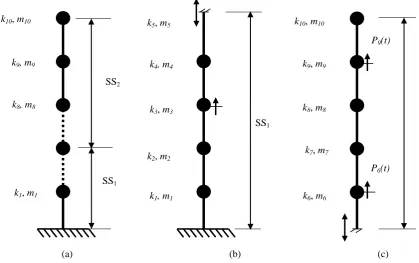
(a) (b) (c) Fig. 3 (a) Full structure (b) substructure SS1 and (c) substructure SS
As shown in Fig. 3 the mass of the structure is lumped at each floor level with masses m
2
1 to m10 and springs of stiffness
k1 to k10. The first substructure (SS1) includes levels up to 5, but the mass at node 5 is not included in the substructure
formation. The second substructure (SS2
Other acceleration sensors are assumed to be placed to obtain response measurements (output) at the second level in first substructure (SS
) starts from level 5 to 10. The substructure interface acceleration at DOF 5 is necessary to be measured as an input to enforce substructure compatibility condition as discussed in section 2.
1) and at seventh and tenth levels in second substructure (SS2) for defining the fitness function (i.e., to
minimize the difference between predicted and measured accelerations at these points). The reason for using one output sensor in SS1 and two output sensors in SS2
In the identification procedure, stiffness k
is to compare the effect of number of sensors on the accuracy of identification.
1 to k5 are the unknown parameters in SS1; similarly k6 to k10 are the unknown
parameters in SS2. The damping parameters α and β are also evaluated using measurements from SS2
To analyze the effect of weighting factor variation in MO, three different weighting factors cases were analyzed in detail for the search. The first case (AP
. The structure is excited with random Gaussian white noise of lower frequency limit of 6 Hz and upper frequency limit of 15 Hz with maximum magnitude 31.5N at third, sixth and ninth levels to excite higher modes,with same damping coefficients of Rayleigh damping model. The responses from 10 to 15 seconds are considered with 0.002 seconds time interval.
1) considers weights of {0.75,0.25}, where first weight represents acceleration matching
(75%) and second weight represents power flow balance matching (25%) respectively. The second case (AP2) considers
weights of {0.5, 0.5} and last case (AP3
Responses and excitations with and without noise contamination are considered first to identify the structural stiffness parameters for each level and damping coefficients of the lumped mass system. For simulation of experimental errors, Gaussian noise with zero mean and 3% standard deviation is added to the time signals of numerically simulated responses.
) considers weights of {0.25, 0.75} respectively. Later a graph (Fig. 5) is shown with data from intermediate weights {0.6, 0.4} and {0.4, 0.6} to show the range of variation.
k1, m1
k9, m9
k10, m10
k8, m8
SS1
SS2
k1, m1
k2, m2
k3, m3
k4, m4
k5, m5
SS1
P9(t)
P6(t)
k6, m6
k7, m7
k8, m8
k9, m9
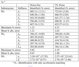
Table 2 Identified Substructure Parameters Using Acceleration Matching A1*
Noise free 3% Noise
Substructure Stiffness Identified (% error) Identified (% error)
SS1 k1 685.11 (-2.13 ) 723.01 (3.29)
k2 640.28 (-1.50) 668.55 (2.85) k3 654.39 (0.685) 641.27 (-1.34) k4 596.88 (-0.52) 608.82 (1.47) k5 607.24 (1.21) 625.27 (4.21)
Maximum % errror 1.21 4.21
Mean % abs. error 1.21 2.63
SS2 k6 396.43 (-0.89) 398.88 (-0.28)
k7 403.30 (0.82) 407.75 (1.94) k8 400.88 (0.22) 416.76 (4.19) k9 297.78 (-0.74) 296.36 (-1.21) k10 302.08 (0.69) 304.14 (1.38)
Maximum % errror 0.82 4.19
Mean % abs. error 0.67 1.80
SS2 α 3.18×10⁻¹ (17.55) 3.57×10⁻¹ (23.61)
β 2.72×10⁻³ (0.37) 2.76×10⁻³ (1.66) *A1
The identified results from only acceleration matching in Table II is compared with the results obtained from multi-objective optimization (MO) of combined acceleration and power flow balance matching in Table III. Table II gives the identified 10 stiffness values and two damping constants for substructures (SS
: Identification with only acceleration matching
1 and SS2
Table III compares the effect of weight factor variation with and without noise contamination for substructural identification. Comparing Table II with Table III it is evident that MO with weighted aggregation technique improves the accuracy of the identified parameters. It may be noted that SS
) with and without noise contamination for only acceleration matching.
1 uses only one sensor whereas SS2 uses two measurement
sensors, which is the reason for obtaining more accurate identified parameters from SS2
The mean absolute error for SS
.
1 and SS2 are 1.21% and 0.67% respectively for only acceleration matching with zero
noise. For the same cases, the respective errors when using combined acceleration and power flow matching, with a weighting factor of {0.5, 0.5} are 0.78% and 0.24% respectively i.e., there is a reduction in mean absolute error of 35.53% and 64.18% for the two substructures. For the 3% noise polluted case the reduction is 36.88% for SS1 and 31.11% for SS2
Now the effect of using different weighting factors is discussed from Table III. For SS
respectively.
1
The mean absolute error corresponding to weight factors {0.5,0.5} for SS
the mean absolute error corresponding to weight factors {0.5, 0.5} is 0.78%, which is less than the errors corresponding to weight factors {0.25,0.75} and {0.75,0.25} for noise free case.
2 is 0.24%, which is again less than the mean
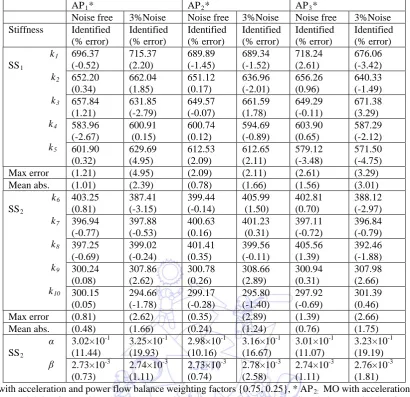
Table 3 Substructure Identification Of Lumped Mass System With Acceleration And Power Flow Balance Matching
AP1* AP2* AP3*
Noise free 3%Noise Noise free 3%Noise Noise free 3%Noise Stiffness Identified
(% error) Identified (% error) Identified (% error) Identified (% error) Identified (% error) Identified (% error) k SS 1 k 1 2 k3 k 4 k5 696.37 (-0.52) 715.37 (2.20) 689.89 (-1.45) 689.34 (-1.52) 718.24 (2.61) 676.06 (-3.42) 652.20 (0.34) 662.04 (1.85) 651.12 (0.17) 636.96 (-2.01) 656.26 (0.96) 640.33 (-1.49) 657.84 (1.21) 631.85 (-2.79) 649.57 (-0.07) 661.59 (1.78) 649.29 (-0.11) 671.38 (3.29) 583.96 (-2.67) 600.91 (0.15) 600.74 (0.12) 594.69 (-0.89) 603.90 (0.65) 587.29 (-2.12) 601.90 (0.32) 629.69 (4.95) 612.53 (2.09) 612.65 (2.11) 579.12 (-3.48) 571.50 (-4.75)
Max error (1.21) (4.95) (2.09) (2.11) (2.61) (3.29)
Mean abs. (1.01) (2.39) (0.78) (1.66) (1.56) (3.01)
k SS 6 k 2 7 k 8 k9 k10 403.25 (0.81) 387.41 (-3.15) 399.44 (-0.14) 405.99 (1.50) 402.81 (0.70) 388.12 (-2.97) 396.94 (-0.77) 397.88 (-0.53) 400.63 (0.16) 401.23 (0.31) 397.11 (-0.72) 396.84 (-0.79) 397.25 (-0.69) 399.02 (-0.24) 401.41 (0.35) 399.56 (-0.11) 405.56 (1.39) 392.46 (-1.88) 300.24 (0.08) 307.86 (2.62) 300.78 (0.26) 308.66 (2.89) 300.94 (0.31) 307.98 (2.66) 300.15 (0.05) 294.66 (-1.78) 299.17 (-0.28) 295.80 (-1.40) 297.92 (-0.69) 301.39 (0.46)
Max error (0.81) (2.62) (0.35) (2.89) (1.39) (2.66)
Mean abs. (0.48) (1.66) (0.24) (1.24) (0.76) (1.75)
α SS β 2 3.02×10 (11.44) -1 3.25×10 (19.93) -1 2.98×10 (10.16) -1 3.16×10 (16.67) -1 3.01×10 (11.07) -1 3.23×10 (19.19) -1 2.73×10 (0.73) -3 2.74×10 (1.11) -3 2.73×10 (0.74) -3 2.78×10 (2.58) -3 2.74×10 (1.11) -3 2.76×10 (1.81) -3
*AP1: MO with acceleration and power flow balance weighting factors {0.75, 0.25}, * AP2: MO with acceleration and power
flow balance weighting factors {0.5, 0.5}, * AP3: MO with acceleration and power flow balance weighting factors {0.25,
0.75}
Fig. 4 Ratio of identified to exact stiffness noise free case (Example 1)
As an illustration, the identified normalized stiffnesses (expressed as the ratio of identified to exact stiffness), without noise contamination are presented in Fig. 4. It shows normalized stiffnesses for k1 to k10, from both substructures with only
acceleration matching (A1) and with combined acceleration and power flow balance matching AP2 (with weight (0.5, 0.5)) for
noise free case. It may be noted that stiffness k1 to k5 are obtained from SS1 and k6 to k10 from SS2. It is seen that results for
stiffnesses k6 to k10 are identified with better accuracy than k1 to k5 because the former comes from SS2 which has 2 output
sensors to match the predicted and measured accelerations whereas SS1
Fig. 5 explains graphically the accuracy of using various combinations of weighting factors. Weighting factors {0.25, 0.75}, {0.4, 0.6}, {0.5, 0.5}, {0.6, 0.4} and {0.75, 0.25} are shown along with mean absolute errors. It is evident that, weight factor corresponding to {0.5, 0.5} gives the least error.
has only one sensor. The same trend is seen for the 3% noisy case from the data in Table III and for brevity is not shown again as a graph.
Fig. 5 Mean absolute errors with different weight factors for SS1
Now the result is compared with those from the original paper [10] from which this example is taken. There the average mean absolute error of 4.0% was noted with only acceleration matching using Genetic Algorithm (for SS
(Example 1)
1 for 3% noisy case).
In the present study (using PSO) the mean absolute error with only acceleration matching in the case of SS1 is 2.63% and with
combined acceleration and power flow balance matching (AP2
6.2. Example 2: 44 DOF planar truss structure divided into four substructures with harmonic excitation ), the respective error reduces to 1.66%.
In this case, the two span planar truss which contains 55 truss elements, 24 nodes and 44 DOFs as shown in Fig. 6, taken from [12,20], is considered for the identification of axial rigidity of the substructure members and Rayleigh damping coefficients. The material and geometric properties of the structure are as follows, the Elastic modulus = 200GPa, the cross-sectional area = 0.03m2 and the mass density = 8000kg/m3 respectively. As the first step of identification purpose the planar truss structure is divided into four substructures (SS1, SS2, SS3 and SS4)as shown Fig. 7. The second substructure (SS3)
from the right end of the full planar truss structure is taken for identification using the proposed method. The substructure to be identified is excited within and outside the substructure by a harmonic force (F1(t) and F2(t)), 15000sin (2 60t) in vertical
direction as per the original papers. The elemental axial rigidity, EA (where E and A represent Young’s modulus and cross-sectional area respectively) of each element (1-16) and damping coefficients α and β are assumed to be unknown for substructure SS3 is presented here.
Fig. 6 Two span planar truss structure (Example 2) F2(t
F1(t
Y
X
12x 10 m
SS1 SS2 SS3 SS4
Numerically simulated responses from 2 to 4 seconds are considered with 0.002 seconds time interval. The natural frequencies of first two global modes of vibration are 5.9037 Hz and 8.3866 Hz respectively. Rayleigh damping model with damping coefficients α = 1.3062 and β = 6.6823×10-04, providing approximately (ζ) 3% damping ratio for the first two modes of vibration are assumed to be known. Numerically simulated response measurement (output acceleration) is assumed to be available at only one node (between elements 2 and 3) inside the substructure from a sensor M, for defining fitness function. The interface response measurements (I1, I2 and I3) are measured using sensors, are also available for evaluating interface
motion forces as shown in Fig. 7. Similar to the first example, both noise free and noisy case of 3% Gaussian noise is considered.
Fig. 7 Two span planar truss structure (Example 2)
Fig. 8 Ratio of identified to exact stiffness with noise free case (Example 2)
The 16 identified normalized axial rigidities of SS3 (expressed as the ratio of identified to exact axial rigidity), without
noise contamination are presented in Fig. 8. Results for only acceleration matching (A1) and combined acceleration and power
flow balance matching (AP2
The identified results of EA for 16 elements and two damping coefficients for acceleration alone matching (A ) are graphically shown, and the improvement in results of the latter case can be observed. The noisy case shows a similar trend as can be seen from the data in Table IV and is not repeated as a graph for brevity.
1) and
combined acceleration and power flow balance matching (AP2) are presented in Table IV for noise free condition and 3%
noise condition. Identification using combined acceleration and power flow balance matching is done only with weight factors {0.5,0.5}, as weighting factors corresponding to AP2 case was found superior to other cases, when compared for the first
example. For the noise free case, the identified mean absolute error for SS3 is 0.62% for only acceleration matching. The
respective error for MO with weight factors {0.5, 0.5} reduces to 0.18%. Thus there is a reduction of 70.96% in mean absolute error. For the noisy case the reduction is 50.80% for SS3. The Rayleigh’s damping parameters are also identified accurately.
SS1
F1(t)
SS2 SS
3
M
16 F2(t)
I1
I2
I3
1 2
3
4 5
6
7 8
9 10
11 12
13
14 15
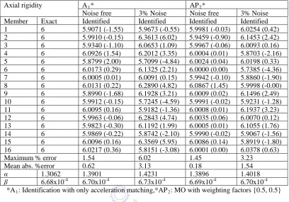
Table 4 Substructure Identification Of Planar Truss With Acceleration Matching And Mo With Weight Factors {0.5, 0.5} Axial rigidity A1* AP2*
Noise free 3% Noise Noise free 3% Noise Member Exact
Identified Identified Identified Identified 1 6 5.9071 (-1.55) 5.9673 (-0.55) 5.9981 (-0.03) 6.0254 (0.42) 2 6 5.9910 (-0.15) 6.3613 (6.02) 5.9459 (-0.90) 6.1453 (2.42) 3 6 5.9340 (-1.10) 6.0653 (1.09) 5.9967 (-0.06) 6.0093 (0.16) 4 6 6.0926 (1.54) 6.2012 (3.35) 6.0004 (0.01) 5.8703 (-2.16) 5 6 5.8799 (2.00) 5.7099 (-4.84) 6.0024 (0.04) 6.0198 (0.33) 6 6 6.0173 (0.29) 6.1325 (2.21) 6.0000 (0.00) 5.7385 (-4.36) 7 6 6.0005 (0.01) 6.0091 (0.15) 5.9942 (-0.10) 5.8860 (-1.90) 8 6 6.0131 (0.22) 6.2890 (4.82) 6.0867 (1.45) 5.9998 (-0.00) 9 6 5.8990 (-1.68) 6.1928 (3.21) 6.0009 (0.02) 6.1496 (2.49) 10 6 5.9912 (-0.15) 5.7245 (-4.59) 5.9991 (-0.02) 5.9231 (-1.28) 11 6 6.0095 (0.16) 5.9182 (-1.36) 6.0008 (0.01) 6.1937 (3.23) 12 6 5.9963 (-0.06) 6.2843 (4.74) 6.0035 (0.06) 6.0070 (0.12) 13 6 5.9823 (-0.30) 6.1192 (1.99) 6.0005 (0.01) 6.1055 (1.76) 14 6 5.9869 (-0.22) 5.8742 (-2.10) 5.9990 (-0.02) 5.9067 (-1.56) 15 6 6.0096 (0.16) 6.3569 (5.95) 6.0086 (0.14) 5.8919 (-1.80) 16 6 6.0217 (0.36) 5.8151 (-3.08) 6.0001 (0.00) 6.0378 (0.63)
Maximum % error 1.54 6.02 1.45 3.23
Mean abs. %error 0.62 3.13 0.18 1.54
α 1.3062 1.3901 1.4231 1.3896 1.4018
β 6.68x10⁻⁴ 6.70x10⁻⁴ 6.73x10⁻⁴ 6.69x10⁻⁴ 6.70x10⁻⁴ *A1: Identification with only acceleration matching,*AP2
Now the result is compared with those of the original paper [12]. There, with 3% noise pollution the mean absolute error for SS
: MO with weighting factors {0.5, 0.5}
3 was 3.08% (it was a least square method based on displacements). In the present study, the respective error with only
acceleration matching is 3.13% and for combined acceleration and power flow balance matching (AP2
6.3. Example 3:A Cantilever beam
) is 1.54%. The results shows that the proposed method of combined acceleration and power flow balance matching can be applied for complex structures with large number of DOFs
The proposed methodis next appliedto a cantilever beam model taken from [12, 21]. The aluminum cantilever beam is 495.3 mm long, 25.4 mm wide and 6.35 mm thickness as shown in Fig. 9 with Young’s modulus 7.1 × 10¹⁰ N/m2 and the mass density is 2.21 × 10³kg/m3. The cantilever beam is modeled with 20 Euler beam elements and divided into four substructures. The second substructure from the right end of the beam is taken for identification using the proposed method. The substructure to be identified is excited within the substructure by a harmonic force (P5(t)), 1.5sin (2 50t) in vertical direction. The
substructure under consideration consist of 5 elements, whose bending stiffness EI (where E and I represent Young’s modulus and Area Moment of Inertia of the cross section respectively) and Rayleigh damping coefficients are treated as unknown. Numerically simulated responses from 2 to 5 seconds are considered with 0.002 seconds time interval. Natural frequencies for first two global modes of vibration are 23.7340 Hz and 148.7386 Hz respectively. Rayleigh damping model with damping coefficients α = 7.7162 and β = 5.5367×10-05
As shown in Fig. 9, interface accelerations are measured at A and B using sensors. Output acceleration measurements are available from a sensor at location M for defining fitness function. In keeping with [12, 21] cases of noise contamination with 1% and 3% Gaussian noise are considered to identify bending stiffness and damping coefficients. The identified results of EI for 5 elements and damping coefficients are presented in Table V.
Fig. 9 Cantilever beam with proposed substructure.
For only acceleration matching, the respective errors are 2.09%, 2.53% and 3.75% for noise free, 1% noise and 3% noise cases. When using MO with weighting factor {0.5, 0.5} these errors are respectively 1.39%, 1.58% and 1.78%. The reductions are respectively 33.49%, 37.55% and 52.53%. However some errors are incurred in the identification of damping coefficients, with the value of α being somewhat fairly identified, but the value of β having more errors.
Now the mean absolute error is compared with the original paper [12] with 3% noise pollution for the same substructure. The observed error in [12] was 4.51% and in the present study the error with only acceleration matching (A1) is 3.75% and for
combined acceleration and power flow balance matching (AP2
Table 5 Substructure Identification Of Cantilever Beam With Acceleration Matching And Mo With Weight Factors {0.5, 0.5} ) is 1.78%.
*A1: Identification with only acceleration matching,*AP2
The above results consistently show that the proposed method of multi-objective optimization with combined power flow balancing and acceleration matching gives more accurate results than pure acceleration matching. In general for all the cases studied the largest errors are observed in the damping coefficients perhaps due to the fact that the damping representations are approximate, so its value is poorly estimated.
: MO with weighting factors {0.5, 0.5}
7.
Conclusions
In this paper, structural parameter identification using a multi-objective optimization (MO) approach with combined acceleration as well as power flow balance matching is studied and compared to only acceleration matching. No extra sensors
Element Number
Exact EI
A1* AP2*
Noise free 1% Noise 3%Noise Noise free 1% Noise 3% Noise Identified Identified Identified Identified Identified Identified
1 38.64 39.02 (0.98) 40.04 39.23 38.16 38.01 37.45
2 38.64 39.80 (2.99) 38.03 37.20 39.37 38.18 39.30
3 38.64 39.81 (3.03) 37.51 37.12 39.16 38.15 39.32
4 38.64 38.46 (-0.48) 37.65 40.90 38.42 39.64 38.90
5 38.64 39.80 (2.99) 37.89 37.21 39.37 38.18 39.30
Maximum % error 3.03 3.62 5.85 1.89 2.59 1.75
Mean abs. % error 2.09 2.53 3.75 1.39 1.58 1.78
α 7.72 10.25 11.57 11.46 11.57 11.57 11.39
β 5.54x10-05 5.58x10-05 5.56x10-05 5.54x10-05 5.69x10-05 5.60x10-05 7.17x10-05
123.83 mm P5(t)
Interface Interface B
25.4 6.35
Substructure 495.3 mm
are required to estimate power flows. This concept of power flow balance is applied to the parameter identification of substructures in the time domain. This combined approach identifies structural parameters with more accuracy compared to conventional acceleration only matching methods. The performance of MO approach with the effect of various weighting factors are studied and results corresponding to weight factors {0.5, 0.5} are found better than other weight combinations. Typically in the large truss example, results of axial rigidity identification of a substructure using MO is superior in accuracy to acceleration based results by 71% and 51% respectively for noise free and noisy cases. The results show that acceleration matching and power flow balance matching concepts can be combined to get improved results in structural identification without any extra effort of using additional sensors.
References
[1] R. H. Lyon and G. Maidanik, “Power flow between two linearly coupled oscillators,” The journal of the Acoustical Society of America, vol. 34, pp. 623-639, 1962.
[2] R. E. D. Bishop and D. C. Johnson, The mechanics of vibration. New York: Cambridge University Press, 1960. [3] K. Shankar and A. J. Keane, “Energy flow predictions in a structure of rigidly joined beams using receptance theory,”
Journal of Sound and Vibration, vol. 185, pp. 867-890, 1995.
[4] K. Shankar and A. J. Keane, “Vibrational energy flow analysis using a substructure approach: The application of receptance theory to FEA and SEA,” Journal of Sound and Vibration, vol. 201, pp. 491-513, 1997.
[5] Z. H. Wang, J. T. Xing and G. Price, “Power flow analysis of intermediate rod/beam systems using a substructure method,” Journal of Sound and Vibration, vol. 249, pp. 3-22, January 2002.
[6] Rajendra Singh and Seungbo Kim, “Examination of multi-dimensional vibration isolation measures and their correlation to sound radiation over a broad frequency range,” Journal of Sound and Vibration, vol. 262, pp. 419-455, May 2003. [7] S. K. George and K. Shankar, “Vibrational energies of members in structural networks fitted with tuned vibration
absorbers,” International Journal of Structural Stability and Dynamics, vol. 9, pp. 269-284, Jun. 2006.
[8] Frank J. Fahy, “Statistical energy analysis: a critical overview,” Proc. Roy. Soc. London, vol. A346, pp. 431–447, 1994. [9] C. G. Koh, L. M. See and T. Balendra, “Estimation of structural parameters in time domain: a substructure approach,”
Earthquake Engineering and Structural Dynamics, vol. 20, pp. 787-801, 1991.
[10]C. G. Koh, B. Hong and C. Y. Liaw, “Substructural and progressive structural identification methods,” Engineering Structures, vol. 25, pp. 1551-1563, Oct. 2003.
[11]C. G. Koh and K. Shankar, “Structural identification method without interface measurement,” Journal of Engineering Mechanics, vol. 129, pp. 769-776, 2003.
[12]S. Sandesh and K. Shankar, “Time domain identification of structural parameters and input time history using a substructural approach,” International Journal of Structural Stability and Dynamics, vol. 9, pp. 243-265, 2009. [13]Ray W. Clough and Joseph Penzien, Dynamics of structures, 2nd ed. New York: McGraw-Hill, 1993.
[14]Kalyanmy Deb, Multi-objective optimization using evolutionary algorithms. Singapore: John Wiley & Sons, 2005. [15]James Kennedy and Russell Elberhart, “Particle swarm optimization,” Proc. IEEE International Conference on Neural
Networks, 1995, pp. 1942-1948.
[16]M. Pant, T. Radha and V. P. Singh, “A simple diversity guided particle swarm optimization,” Proc. IEEE Congress. Evolutionary Computation (CEC 2007), Sep. 2007, pp. 3294-3299.
[17]Qie He and Ling Wang, “An effective co-evolutionary particle swarm optimization for constrained engineering design problems,” Engineering Applications of Artificial Intelligence, vol. 20, pp. 89-99, May 2006.
[18]Sidhartha Panda and Narayana Prasad Padhy, “Comparison of particle swarm optimization and genetic algorithm for FACTS- based controller design, ” Applied Soft Computing, vol. 8, pp. 1418-1427, 2008.
[19]C. R. Mouser and S. A. Dunn, “Comparing genetic algorithm and particle swarm optimization for inverse problem,” ANZIAM Journal, vol. 46, pp. 89-101, 2005.
[20]Chung-Bang Yun and Eun Young Bahng, “Substructural identification using neural networks,” Computers and Structures, vol. 77, pp. 41-52, Apr.2000.
[21]Hong Hao and Yong Xia, “Vibration based damage detection of structures by genetic algorithm,” Journal of Computing in Civil Engineering, vol. 16, pp. 222-229, July 2002.