Development of a Prototype Smart City System for Refuse Disposal Management

(1)

http://www.sciencepublishinggroup.com/j/mcs doi: 10.11648/j.mcs.20190401.12

ISSN: 2575-6036 (Print); ISSN: 2575-6028 (Online)

Development of a Prototype Smart City System for Refuse

Disposal Management

Joke O. Adeyemo

*

, Oludayo O. Olugbara, Emmanuel Adetiba

ICT and Society Research Group, Durban University of Technology, Durban, South Africa

Email address:

*_{Corresponding author}

To cite this article:

Joke O. Adeyemo, Oludayo O. Olugbara, Emmanuel Adetiba. Development of a Prototype Smart City System for Refuse Disposal Management. Mathematics and Computer Science. Vol. 4, No. 1, 2019, pp. 6-23. doi: 10.11648/j.mcs.20190401.12

Received: August 20, 2018; Accepted: October 6, 2018; Published: May 15, 2019

Abstract:

The future of modern cities largely depends on how well they can tackle problems that confront them by embracing the next era of digital revolution. A vital element of such revolution is the creation of smart cities. Smart city is an evolving paradigm that involves the deployment of information communication technology wares into public or private infrastructure to provide intelligent data gathering and analysis. To align concretely with the smart city revolution in the area of environmental cleanliness, this paper involves the development of a smart city system for refuse disposal management. The architecture of the proposed system is an adaptation of the Jalali reference smart city architecture. It features four essential layers, which are signal sensing and processing, network, intelligent user application and Internet of Things (IoT) web application layers. A proof of concept prototype was implemented based on the designed architecture of the proposed system. The signal sensing and processing layer was implemented to produce a smart refuse bin that contains the Arduino microcontroller board, Wi-Fi/GSM transceiver, proximity sensor, gas sensor, temperature sensor and other relevant electronic components. The network layer provides interconnectivity among the layers via the internet. The intelligent user application layer was realized with non-browser client application, statistical feature extraction method and pattern classifiers. Whereas the IoT web application layer was realised with ThingSpeak, which is an online web application for IoT based projects. The sensors in the smart refuse bin generate multivariate dataset that corresponds to the status of refuse in the bin. Training and testing features were extracted from the dataset using first order statistical feature extraction method. Afterward, multilayer perceptron artificial neural network and support vector machine were trained and compared experimentally. The multilayer perceptron artificial neural network model gave the overall best accuracy of 98.0% and the least mean square error of 0.0036.

Keywords:

Disposal, Embedded, Feature Extraction, IoT, Pattern Classifier, Smart City

1. Introduction

The International Telecommunications Union (ITU) describes a smart city as an innovative city that uses Information Communication Technology (ICT) and other means to improve the quality of life of the citizens [1]. There have been various initiatives and studies about smart cities by multinational companies and research institutes with the aim of making cities smarter through effective utilization of available resources [2]. Smart city projects primarily rely on data gathering from the city infrastructure. Such data include weather information, electrical energy consumption pattern and refuse disposal infrastructure usage to mention just a few

[3, 9].

Most communities across the globe are experiencing serious budgetary challenges on refuse disposal [4, 5]. Despite the provision of refuse bin within most municipalities, the fundamental responsibility to maintain a culture of environmental sanitation is left in the hands of individuals. There are also challenges with respect to collection services. Consequently, refuse bins often spill over into accumulation. An environmental cleanliness solution is therefore mandatory for any community seeking progress in the well-being of its populace [5].

(2)

refuse accumulation problems [6-8]. Collection services can therefore be more effective through an automated alert procedure that readily indicates refuse bin status and prompt response for refuse collection based on such alert can help to promote long term communal sanitation.

The requirements of a smart refuse disposal system include system simplicity, cost effectiveness, easy management, flexibility and portability [9]. Smart refuse disposal systems should also be able to make automatic decision with respect to the status of the refuse bin with little or no input from humans [10-11]. Hence, the aim of this study is to develop smart city technology based system architecture and prototype for refuse disposal management. Based on this overarching aim, the objectives of the study are: a) To provide timely and accurate information on the status of refuse bins to the relevant refuse disposal management agents. b) To enhance the ease with which full refuse bins are located by refuse collection agents.

Related Works

Refuse management is obviously a concern in modern cities because of service cost and storage problem that are associated with disposing refuse in landfills. Published works from researchers have indicated different ways that technology have been applied in an attempt to achieve smart refuse disposal management.

The Wireless Sensor Networks (WSN), Global System for Mobile Communications (GSM) and Radio Frequency Identification (RFID) technologies have been employed by authors to develop smart refuse disposal management systems. For instance, real time activity monitoring system for waste bins was developed by Chowdhury and Chowdhury [13]. The systems is based on multi-tier platform of wireless sensors and RFID technology. The authors utilised knowledge driven database to filter sample datasets and an extensible graphical user interface for user friendliness. Bashir et al. [14] designed a vehicular smart transport using Infra-Red sensor, radio frequency encoder along with decoder base station nodes for smart bin monitoring. The system ensures that refuse collection service agents are accountable through data entry for bin status and location. Longhi et al. [15] proposed a method to determine smart bin position via a wireless sensor unique received signal strength information. According to the authors, the work was aimed at improving the accuracy in bin activity monitoring by means of a public open sensor innovation. Glouche et al. [16] proposed a new approach by using RFID on smart bin. The refuse items were configured as self-describing objects as a quick option for easy recycling.

Moreover, pattern recognition algorithms have also been recently employed to realise refuse disposal management. Abbasi et al. [17] developed a method for forecasting Municipal Solid Waste (MSW) generation. The researchers combined the Support Vector Machine (SVM) classifier and Partial Least Square (PLS) for feature selection to determine the quantity of MSW that are generated on a weekly basis in Tehran, Iran. Comparing SVM and PLS-SVM models, the authors reported that PLS-SVM gave superior performance

to the SVM model with respect to predictive ability and computational time. Livani et al. [18] developed a prediction method in which the weighted K-means clustering algorithm was utilized for clustering refuse dataset of 63,000 records. Afterwards, linear regression model was used to build the prediction models from each of the clusters. They submitted that the combination of the two methods gave better performance than using each of the methods individually. Additionally, the authors produced a hybrid of the prediction model to develop a decision support system for refuse collection and recycling services.

Essentially, Nuortio et al. [19] and Zanella et al. [20] are of the opinion that through the use of smart bin that can detect load level and allow collector truck route optimization, cost reduction and improved quality of the refuse management service can be achieved.

2. Materials and Methods

The various smart city architectures in the literature contains Radio Frequency (RF) components and sensors, liaison networks as well as service-oriented information systems as the first, second and third layers respectively [20-23]. A vital gap in those earlier architectures is the lack of specific intelligent data processing in the service–oriented information system layer. The topologies of most of the architectures are also cumbersome, which may impose some difficulties for practitioners that desire to implement them. These gaps provide the motivation to develop a system architecture in this study, which is an adaptation of the Jalali et al. (2015) smart city reference architecture for refuse disposal management.

The proposed architecture (Figure 1) is more compact than the reference architecture Jalali et al. [25] and it incorporates pattern recognition methods for bin status decision making. The compactness provides ease of implementation for the architecture while the pattern recognition methods provide better decision by processing multivariate dataset extracted from the internal state of the refuse bin. The four layers in the proposed architecture are the Signal Sensing and Processing Layer (SSPL), Intelligent User Application Layer (IUAL), IoT Web Application Layer (IWAL) and the Network Layer (NL). The NL provides wide area wireless communication channel for the other three layers using the Internet technology. However, each of the other three layers (SSPL, IUAL and IWAL) offers a template for the design of the functional hardware and software units of the prototype in this paper.

2.1. Signal Sensing and Processing Layer of the Proposed Architecture

(3)

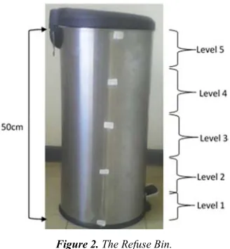
is calibrated into five different levels as shown in Figure 2. Level1, level2, level3, level4 and level5 represent empty, quarter-full, half-full, three-quarter-full and full statuses respectively. The PSU contains rectification circuits to convert Alternating Current (AC) from the main supply to Direct Current (5V DC), which powers the SSPL. The electronic sensors capture raw information from the RB and

transduce them into electronic signals. Such signals include: The distance from the lid to the level of refuse in the RB using proximity sensor.

The gaseous emission from the decomposing refuse using gas sensor.

The temperature of the refuse in the RB using temperature sensor.

Figure 1. The proposed smart refuse disposal system architecture.

Figure 2. The Refuse Bin.

The microcontroller in the SSPL was realised with an Arduino microcontroller board. The Arduino board contains

an ATmega328 microprocessor, memory interface

controllers, timers, interrupt controller and General Purpose Input/Output (GPIO) pins. Six electronic sensors were

utilised in the SSPL. These include two Sharp

GP2Y0A02YK0F proximity sensors, two MQ 135 gas sensors and two LM35 temperature sensors (GP2Y0A02YK0F Datasheet, MQ135 Datasheet, and LM35 Datasheet). The six sensors have three pins - Vcc, GND and Vo, which are connected using male and female jumper wires to the 5V, GND and Analog pins 0, 1, 2, 3, 4 and 5 respectively on the microcontroller board. The duplication of each of the sensors is to incorporate redundancy into the SSPL circuitry, eliminate data sparsity and provide holistic coverage of the entire RB.

(4)

is produced from refuse is methane [26]. The LM35 temperature sensor operates from 4V to 30V. This implies that the sensor can be powered conveniently from any of the microcontroller’s power pins. It is calibrated directly in Celsius with linear +10-mV/°C scale factor and rated for full −55°C to 150°C. The characteristic curve in the datasheet [27] shows that the functioning of the temperature sensors exhibit a positive exponential behavior over time. While the refuse get decomposed in the RB, microorganisms consume the organic matter and generate both heat and other gases. Once the temperature sensors are powered, they read the internal heat within the RB. Because the RB was located in the laboratory for this work (being a prototyping phase), the heat will largely depend on the quantity of refuse in the bin.

The GSM/GPRS or Wi-Fi transceiver in Figure 1 provides optional internet access for the SSPL to transmit data stream to the IoT web application (which will be discussed later in this section). The transmitted data stream contains information concerning the status of the refuse in the RB. Nevertheless, the Wi-Fi interface card on the development PC was used to emulate a Wi-Fi transceiver for connecting the microcontroller board to the internet wirelessly. The Wi-Fi option became paramount because using a GSM/GPRS transceiver is too cost intensive for a work of this nature, since the mobile operators require the GSM/GPRS transceiver to always have data subscription in order to gain connection to the internet. However, the GSM/GPRS transceiver option will be very handy for real-time deployment, which is beyond the scope of the current study. The SSPL circuitry is incorporated into the RB shown in Figure 2 to produce the Smart Refuse Bin (SRB). The pictorial view of the SRB is presented in Section 3.

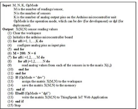
The ATmega328 microprocessor translates the electrical signals from the sensors into digital data streams using the embedded program in the memory of the microcontroller. The algorithm of the embedded program is shown in Algorithm 1. The algorithm was implemented using the Arduino hardware support package in MATLAB R2015a and loaded into the microcontroller for full functionality.

Figure 3. Embedded program of the microcontroller unit.

2.2. IoT Web Application Layer of the Proposed Architecture

The IoT Web Application Layer (IWAL) shown in Figure 1 is primarily made up of IoT based web application services and protocols. Internet of Things (IoT) is a technological scenario in which connected systems acquire, process, store or communicate data gathered by electronic sensors from machines, objects, environments, infrastructure and other physical entities. The data is thus processed into beneficial information that can be applied to “command and control” things to improve human lives on the planet [29-30]. Some examples of IoT web applications are ThingsSpeak, Carriots, SmartObject, Skynet Sensorthings, Nimbits, SensorCloud, Exosite, iDi, EVRYTHNG, Paraimpu, Manybots and Pachube [31-32]. ThingSpeak is selected for this work out of these numerous IoT web applications because of its notable advantages and strengths.

ThingSpeak is an open source IoT web application which uses Phusion Passenger Enterprise web application server. It provides Application Programming Interfaces (APIs) for storing and retrieving data from sensors and devices over the internet. According to Maureira et al. [32], the servers being used by some of the other IoT applications are not clearly documented. Another clear advantage of ThingSpeak that motivates its selection for this work is that its APIs provide support for programming languages such as Ruby, Python, MATLAB and Node.js.

Furthermore, ThingSpeak also provides free hosting for data channels. Each channel in ThingSpeak support data entries of 8 data fields, latitude, longitude, elevation, description and status. Incoming data from sensors into the channels are communicated via Hyper Text Transport Protocol (HTTP) POSTs through plaintext, JASON or XML formats. The channels are set to private by default and machines or users need read or write key, which is generated by ThingSpeak to access the data [31-32].

Given the above mentioned strengths of ThingSpeak over its rivals, the writing/reading of sensors’ data to/from ThingSpeak were implemented in this study with functions in the ThingSpeak Support Toolbox for MATLAB R2015a. The results obtained are presented in Section 3.

2.3. Intelligent User Application Layer of the Proposed Architecture

(5)

2.3.1. Dataset and First Order Statistical Feature Extraction

To obtain the training and testing data sets for this work, the authors collected wastes from refuse containers that are located within the Ritson Campus at the Durban University of Technology, South Africa. The refuse containers contain decomposing materials, papers and different varieties of solid wastes that were dumped by students, staff as well as visitors within the University. The embedded program within the microcontroller of the SRB extract data in 200 iterations from each of the 6 sensors to produce a 200x6 dataset for each level of the SRB. The procedure for generating the data sets using the embedded program has been presented in Algorithm 1. Data were extracted in 200 iterations to cater for any possible electrical variation within the sensors.

Irrefutably, pattern classification using original sensor measurements is often inefficient and may even hinder proper interpretation [34]. Feature extraction therefore reduces the dimensionality of raw dataset by keeping the

most discriminatory information. In addition, the

performance of the feature extraction stage sturdily impacts the design and performance of pattern classifiers. If the best features are selected from the raw data, the task of the subsequent pattern classifiers becomes trivial. Conversely, if the features with little discriminatory ability are chosen, a more complex pattern classifier may be required [35].

Principal Component Analysis (PCA) is one of the most commonly used algorithms for features extraction and dimensionality reduction in fields like image processing, pattern recognition, bioinformatics, telecommunications and etcetera. It is an optimal linear transformation algorithm for keeping the subspace of a dataset that has the largest variance. However, the computational requirement for PCA is high [34] [36-37]. First Order Statistical Features (FOSF) is another strategy being employed for discriminatory features extraction with lower computational requirements (Indonesia 2011). The computational advantage of the FOSF over PCA motivate its selection as the feature extraction method for this research work.

The FOSF utilised include the mean, standard deviation, kurtosis and skewness values computed from each of the 200 values generated for each of the 6 sensors per SRB level [34, 37-38]. The computed mean, standard deviation, skewness and kurtosis for the six sensors were concatenated to obtain FOSF vectors in 24- dimensional space for each level of the smart refuse bin. The procedure for computing the FOSF was

implemented in MATLAB R2015a programming

environment.

2.3.2. Pattern Classification

The feature vectors obtained with the FOSF extraction method discussed in the preceding sub section is transmitted to train the selected pattern classifiers. A trained pattern classifier will thus be able to categorise an incoming raw data stream from the SSPL, which have been processed with the FOSF into one of empty, quarter full, half full, three quarter full and full bin status.

Two state-of-the-art pattern classifiers investigated for the classification of the features in this work are the Multilayer Perceptron Artificial Neural Network (MLP-ANN) and Support Vector Machine (SVM). They are extensively engaged in the literature to solve pattern classification problems [42]. Nevertheless, each of the classifiers have inherent merits and demerits. MLP neural networks have the capability to detect complex non-linear associations between variables, they are very fast to use for classification problems and generally achieve good performance. However, because MLP is based on the traditional empirical risk minimization principle, it often suffers from overfitting and multiple local minimal. Conversely, SVM has the advantage of good generalization performance because it is based on the structural risk minimization principle. It has a modest geometric interpretation, its computational involvedness do not depend on the dimensionality of the input space and its solution is global and unique. SVM is however a shallow model and its performance result rely heavily on the selected kernel function. The joint strength of both MLP and SVM is that they yield good performance in high-dimensional classification problems. Generally, the best classifier for a given problem depends on the problem domain, the number of classes to be classified and the number of example(s) available per class. Furthermore, experimentation becomes handy to compare the performances of the selected classifiers for this work [39-41].

2.3.3. Configuration of the Pattern Classifiers

The MLP-ANN and SVM were tuned in this study through established parameters in the literature as well as via experimentations to determine the configuration that gives the most optimal performance [33, 42].

(6)

performance record [33] [44-45]. The FOSF were partitioned based on a data partitioning ratio of 70% training, 15% validation and 15% testing. The MLP-ANN contains additional configurations as follows:

Training epochs = 10,000, Learning rate = 0.1,

Maximum training time = 180sec, Minimum performance gradient = 1e-6, Validation checks = 10,000

SVM possesses the ability to capture both linear and nonlinear patterns in feature space by employing a mapping function which transforms the feature space into a higher domain that exhibits multiple dimensionalities [46]. The mapping function is usually implemented by using specialised kernels. Minh et al. (2006) opined that SVM kernels must satisfy Mercer condition for it to be effective. Examples of kernels that satisfy the Mercer condition are linear, polynomial, radial basis function and perceptron kernels [48]. Since the performance of the SVM is determined by the choice of kernel selected for the experiment, the four listed kernels were tested using 10 fold cross validation and their performances were compared. The multi-class SVM techniques that was employed for this study is the One-Against-All (1AA) because it is acclaimed to be simple and highly efficient [48]. The same data partitioning strategy for MLP-ANN was used for training the SVM.

Implementation, training as well as all the experimental configurations of the MLP-ANN and SVM pattern classifiers in this work were carried out in MATLAB R2015a. The computer system for the implementation and experiments contains Intel Core i5-2540MCPU @2.60GHz speed with 4.00GB RAM and 64-bit Windows 8 operating system.

2.3.4. Client Application Design

In this study, the client application, which is a graphical user interface (non-browser-based) web client, was designed with the Universal Modelling Language (UML). UML2 defines 13 basic diagram types that are divided into two generic groups, namely behavioral and structural modeling diagrams. Behavioral diagrams are used to capture the interactions and state instantiations within a model over its execution time. On the other hand, structural diagrams are used to emphasize the things that must be present in the software application being modeled. These include classes, objects and interfaces. Structural diagrams are also used to represent the relationships and dependencies between the various elements of the modeled software [49]. According to Bell [50], the most useful standard UML diagrams are use case, class, sequence, statechart, activity, component and deployment diagrams. However, four of these diagrams sufficiently captures the different views of the IUAL client application as well as the prototype of the proposed architecture (Figure 1). Hence, in this study, use case diagram was used to model the behavioral view while class diagram was used to model the structural view of the client application. Furthermore, activity diagram was adopted to model the operational step-by-step workflow of the hardware

and software components of the full prototype. Deployment diagram was also adopted to model how the entire prototype can be deployed, even though, the deployment of the prototype is beyond the scope of the current study. Nevertheless, due to space constraint, only the activity diagram is described in this paper.

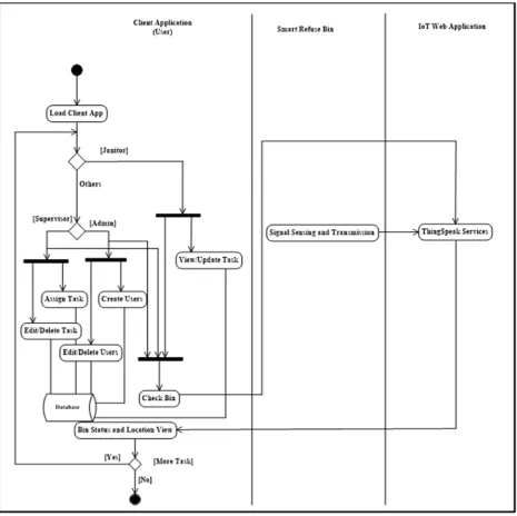
Activity diagram illustrates the flow of signal across the different aspects of a system. It usually consist of shapes such as round-cornered rectangle, diamond, circle, can and interconnection lines, which symbolise action state, decision, start or stop, database and association respectively [49]. Figure 3 shows the activity diagram of the proposed architecture’s prototype. The diagram consists of 10 action states, 3 decisions, 3 forks, 1 database, 1 start and 1 stop symbols. The operation of the entire activity diagram starts with the loading of the client application in the Load Client App action state. A decision on the appropriate user group is taken, which branches out to Janitor and Others. The Janitor user group branches out to 2 action states namely, View/Update Task, and Check Bin. The second decision symbol splits into the Administrator and Supervisor user groups. The Administrator user group links to action states, which are Create Users and Edit/Delete Users. The Supervisor also links to 2 action states, namely Assign Task and Edit/Delete Tasks. Similar to Janitor, both the Administrator and Supervisor also link to the Check Bin action state. The Smart Refuse Bin section has only 1 Signal Sensing and Transmission action state which sends refuse status and location data into the ThingSpeak Services action state at the IoT Web Application section. The ThingSpeak Services action state transmits the data it receives to the Bin Status and Location View action state for the Administrator, Supervisor and Janitor to view the status and location of the SRB. The last decision symbol is for the different user group to determine if more tasks should be performed or all activities should end. If more tasks are desired by any of the user group, a link is returned back to the first decision symbol and there is a link to end the activities if otherwise.

2.4. Performance Evaluation

In order to compare pattern classifiers, it is important to define and specify the evaluation metrics. The performance evaluation metrics of accuracy and Mean Square Error (MSE) were adopted in this work for the MLP-ANN and SVM because they are commonly used in the literature. The accuracy is the degree of closeness of the measurements of a quantity to its true value. Whereas MSE is the mean of the square of the difference between the expected output and the actual output [42, 51].

(7)

are the developers in the context of this work. Unit testing is mostly engaged to test the functionality and quality of software components or a collection of components because it allows easy identification of bugs within the code [54]. Unit testing was realized in this work using the xUnit-style

MATLAB unit testing framework in MATLAB R2015a. Although the researcher is aware of other unit testing frameworks such as MS Test, JUnit and NUnit, the xUnit-style framework becomes handy because all the codes in this work were implemented using MATLAB R2015a.

Figure 4. Activity diagram of the system prototype.

3. Results

3.1. Hardware Unit

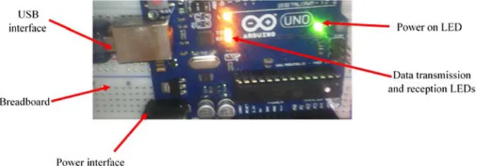
The testing results of the electronic sensors and the arduino microcontroller development board while the prototype is being developed in the laboratory are presented in this sub-section. The Arduino Uno development board, which contains the ATmega 328 microcontroller was connected through USB 2.0 cable to the development PC to evaluate its functionality. The board gets powered up by the

5V voltage that is supplied to it from the PC via the USB 2.0 cable. The On LED situated on the board emits a steady green light to indicate the device is in good and proper working conditions as shown in Figure 4.

(8)

application at the operational phase are deemed successful once the amber coloured LED are on. It is noteworthy that

the pins on the Arduino Uno board connect directly to the corresponding pin on the ATmega 328 microcontroller.

Figure 5. Arduino development board at ready state and TX/RX states.

The functionality of the proximity, gas and temperature sensors were evaluated by connecting them to the appropriate pins on the Arduino board and capturing the sensors’ readings at different levels of the SRB. The plots of the mean voltages obtained from each of the sensors against the distances marked on the SRB are shown in Figure 5. The graph of the proximity sensor is highly similar to the characteristics curve of the sensor in the datasheet, in which

the voltage output was plotted against distance

(GP2Y0A02YK0F Datasheet). The graph of the gas sensor indicates an initial spike at level 1 but reduces drastically and almost remains constant thereafter. The spike is obviously due to high gaseous concentration at that level. This behaviour may also be obtained in real life scenario if the initial refuse that was dumped in the bin contains

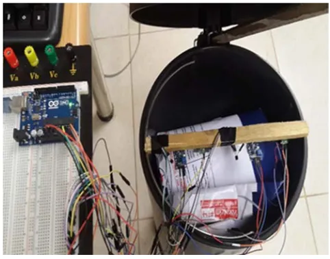
decomposing waste while those that were dumped afterwards until the bin is full have minimal decomposing refuse. The temperature sensor graph also peaked at level 1 but reduces steadily to lower values at level 2 and beyond. With this graph, it can be deduced that the initial refuse in the bin generated more heat since more gaseous emission was also indicated by the gas sensor. As the concentration of the gas reduced, the heat also reduced up to level 2 and afterwards. The test results that were obtained from the three sensors apparently illustrate that they are all suitable for acquiring the appropriate signals, which represent the status of the refuse in the SRB. The SRB picture, showing the refuse bin, microcontroller board, sensor array and connection wires, as it was been constructed in the laboratory is shown in Figure 6.

Figure 6. Mean voltage against the bin levels.

3.2. Software Units

This sub-section presents the configuration, experimental evaluation, implementation and unit testing of the prototype’s software units.

3.2.1. ThingSpeak Configuration

In order for the ThingSpeak web application to be ready for use, a user account was first of all created with username and password. Thereafter, a channel of six fields was created and configured to accept data from each of the six sensors in

1 1.5 2 2.5 3 3.5 4 4.5 5

0 0.5 1 1.5 2 2.5

Bin level

Me

a

n

v

o

lta

g

e

o

f

th

e

s

e

n

s

o

rs

Proximity sensor Gas sensor

(9)

the SRB. Figure 7 shows the home page of a fully configured and customized ThingSpeak web application for this work. The page contains a generic menu bar at the top, which contains the commands that were used for the configuration. After the menu bar, there are labels such as Page title, ChannelID, Author and Access. It also contains link tabs in the middle with labels; Private View, Public View, Channel Settings, API Keys, Data Import/Export. After this, there are clickable buttons such as Add Visualization, Data Export, MATLAB Analysis and MATLAB Visualization. The bottom of the page contains the Channel Stats. There are 200 entries indicated under the Channel Stats for each of the six fields. This clearly illustrates that the data from the SRB were successfully streamed to the ThingSpeak web application. The Access option was initially set to public in order to test the functionality of the application. However, it was eventually set to private in order to secure the data and settings for this research on the ThingSpeak web application

domain on the internet.

Figure 7. SRB construction in the laboratory.

Figure 8. The customised home page on ThingSpeak web application.

The streamed data from the SRB to each of the data fields are graphically captured as shown in Figure 8. Each graph shows the real-time streaming of data from each of the sensors with values on the Y axis and the date/time stamps on the X axis. The data from each sensor were fully available in the ThingSpeak web application within 90 seconds. This

(10)

(11)

Figure 10. Dataset histogram of the first instance of each SRB level.

3.2.2. Acquired Dataset from the Smart Refuse Bin

The SRB is configured to generate 200 values for each of the six sensors so as to produce a 200x6 dataset. However, to acquire sufficient data that caters for possible variations in the electronic sensors while taking the measurement, the researcher deemed it necessary to run several trials for the data acquisition. Overall, there were 15 different data acquisition trials for each of the 5 levels in the SRB (i.e. empty, quarter full, half full, three quarter full and full). This implies that for each bin level, there were 15 different instances of the 200x6 dataset. The entire dataset cannot be presented here because of the huge size. However, to grasp a graphical view of a portion of the data, the histogram plots of the first training instance for each level is presented in Figure 9. The histogram plots, which represent the distribution of the dataset, clearly show that the acquired data are different for each of the levels. For instance, the distribution of the data with high frequencies are concentrated at the middle for level 1 and it contains unique values from 0.1 up to 2.3 with 0.5 having the highest frequency of about 320. Even though the distribution of the data with the highest frequencies are majorly skewed to the left for level 2, level 3, level 4 and

level 5, the range of the data distributions and the frequencies within the range are uniquely different. However, the raw dataset could not be used to train the pattern classifiers directly so as to avoid structural complexity, high computational time, overfitting as well as the curse of dimensionality [34, 42].

3.2.3. First Order Statistical Features

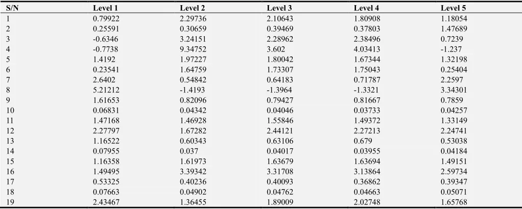
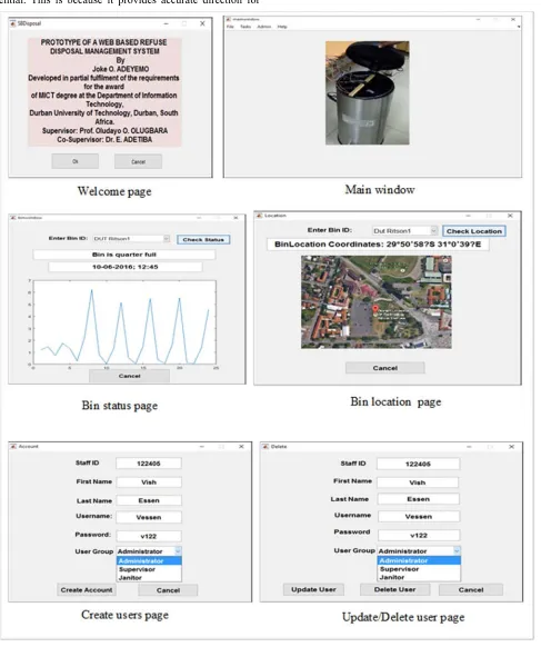
The first order statistics which include mean, standard deviation, skewness and kurtosis were employed to compute discriminatory features from the extracted dataset in this work. These values were computed for each level of the SRB and for all the 15 instances. Due to space constraint, the computed values for the first instances of all the levels are shown in Tables 1. The 4 statistical values were concatenated for all the 6 sensors, which culminated in a feature vector of 24 elements per level. Meanwhile, 10 instances of the feature vectors for each level were earmarked to train the pattern classifiers. The remaining 5 instances were reserved to test the pattern classifiers after they were successfully trained. This strategy helped to examine the generalization ability of the selected pattern classifiers.

Table 1. First order statistical features for the first training instance of each level.

S/N Level 1 Level 2 Level 3 Level 4 Level 5

1 0.79922 2.29736 2.10643 1.80908 1.18054

2 0.25591 0.30659 0.39469 0.37803 1.47689

3 -0.6346 3.24151 2.28962 2.38496 0.7239

4 -0.7738 9.34752 3.602 4.03413 -1.237

5 1.4192 1.97227 1.80042 1.67344 1.32198

6 0.23541 1.64759 1.73307 1.75043 0.25404

7 2.6402 0.54842 0.64183 0.71787 2.2597

8 5.21212 -1.4193 -1.3964 -1.3321 3.34301

9 1.61653 0.82096 0.79427 0.81667 0.7859

10 0.06831 0.04342 0.04046 0.03733 0.04257

11 1.47168 1.46928 1.55846 1.49372 1.33149

12 2.27797 1.67282 2.44121 2.27213 2.24741

13 1.16522 0.60343 0.63106 0.679 0.53038

14 0.07955 0.037 0.04017 0.03955 0.04184

15 1.16358 1.61973 1.63679 1.63694 1.49151

16 1.49495 3.39342 3.31708 3.13864 2.59734

17 0.53325 0.40236 0.40093 0.36862 0.39347

18 0.07663 0.04902 0.04762 0.04663 0.05071

(12)

S/N Level 1 Level 2 Level 3 Level 4 Level 5

20 4.85811 1.74582 4.58913 4.74427 2.66225

21 0.53723 0.1368 0.13356 0.11932 0.12775

22 0.07701 0.05264 0.05377 0.05118 0.05825

23 2.30185 1.59718 1.57779 1.33749 1.38151

24 4.29572 3.28227 4.18363 2.07824 1.66323

3.2.4. Pattern Classifiers Training

The basic configurations of the classifiers as well as the motivation for the choice of the evaluation metrics have been presented in Section 2. As shown in Table 2, the

one-per-class coding method was used to encode the MLP-ANN target output while decimal values were used for the SVM target output [48, 53].

Table 2. Target output of the MLP-ANN and SVM classifiers.

Level Bin Status MLP-ANN Target Output SVM Target Output

1. Empty 1 0 0 0 0 1

2. Quarter Full 0 1 0 0 0 2

3. Half Full 0 0 1 0 0 3

4. Three Quarter Full 0 0 0 1 0 4

5. Full 0 0 0 0 1 5

The first order statistical features earlier computed were used to train the MLP-ANN and SVM classifiers and the outcome of the trainings were evaluated using the accuracy and Mean Square Error (MSE) metrics. The performance results of the trained MLP-ANN for 20, 40, 60, 80 and 100 neurons in the hidden layers are reported in Table 3, while the results of SVM for polynomial, linear, RBF and perceptron kernels are shown in Table 4.

Table 3 shows that the MLP-ANN with 60 neurons in the hidden layers produced the best result among other MLP-ANN configurations with an accuracy of 98% and a MSE of 0.0036. Table 4 also shows that the SVM classifier with polynomial kernel functions gave the highest accuracy among the other SVM kernel functions, with an accuracy of 88.89% and MSE of 0.1558. The MLP-ANN with 60 neurons in the hidden layers is therefore nominated as the pattern classifier for this work based on its superior performance over the others.

Table 3. Performance result of the MLP- ANN pattern classifier.

ANN Type Number of Hidden

layer neurons Accuracy (%) MSE

ANN1 20 94 0.0322

ANN2 40 96 0.0171

ANN3 60 98 0.0036

ANN4 80 98 0.0168

ANN5 100 98 0.0191

Table 4. Performance result of the SVM pattern classifier.

Kernel Accuracy MSE

Polynomial 88.89 0.1558

Linear 77.78 0.1519

RBF 22.22 0.1920

Perceptron 44.44 0.1557

The confusion matrix of the nominated MLP-ANN pattern classifier is shown in Figure 10 to illustrate its performance for each class in the training dataset. The 10 training instances in each of the 1st, 2nd, 4th and 5th classes were correctly classified. However, 9 of the training instances in

the 3rd class were correctly classified while 1 instance was wrongly classified as belonging to the 2nd class. The sum of the percentages of correctly classified classes across the diagonal culminated in the 98% accuracy earlier reported in Table 3.

Figure 11. Confusion matrix of the best MLP-ANN in Table 3.

3.2.5. Testing of the Best Pattern Classifier

(13)

Notably, level 4 was wrongly classified as level 3 in all cases. Assuming the decision for refuse collection is taken when the classification output produces level 5 (full status), it can therefore be stated that the wrong classification of level 4 (three quarter full) as level 3 (half full) does not have any major negative implication. For example, wrongly classifying level 4 (three quarter full) as level 5 (full status) would have

resulted in more adverse effects like wasted effort, time and resources by the refuse collection agents. Essentially, since only one level was wrongly classified for all the testing instances, it can be inferred that the nominated MLP-ANN generalizes well on unseen dataset. The performance of the nominated pattern classifier for this work is therefore adequate and acceptable.

Table 5. Testing result of the best MLP-ANN using the first testing instance.

Level Bin status Expected output Actual output Remark

Level 1 Empty 1 0 0 0 0 1 0 0 0 0 Correct

Level 2 Quarter Full 0 1 0 0 0 0 1 0 0 0 Correct

Level 3 Half Full 0 0 1 0 0 0 0 1 0 0 Correct

Level 4 Three Quarter Full 0 0 0 1 0 0 0 1 0 0 Incorrect

Level 5 Full 0 0 0 0 1 0 0 0 0 1 Correct

Table 6. Testing result of the best MLP-ANN using the second testing instance.

Table 7. Testing result of the best MLP-ANN using the third testing instance.

Table 8. Testing result of the best MLP-ANN using the fourth testing instance.

Table 9. Testing result of the best MLP-ANN using the fifth testing instance.

3.2.6. Client Application Implementation and Unit Testing

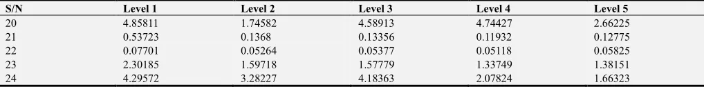
The non-browser client application was implemented in a prototype form using the GUIDE in MATLAB R2015a. The implementation is based on the UML design described in Section 2. Some of the key pages in the implemented application are shown in Figure 11. These include Welcome page, Main window, Bin status page, Bin location page, Create user page and Update/Delete user page. Appropriate codes were written to ensure that all the interfaces perform the functions in the requirement specifications. The manual testing of the functionality of the different commands in all the interfaces to ensure the integrity of the codes was

successful.

(14)

bin status information, the location information is also very essential. This is because it provides accurate direction for

the Janitor to locate bins that are ready for collection.

Figure 12. Client application implementation interfaces.

The output of the unit test carried out for the components of the client application is shown in Figure 12. All the modules in the client application passed the test successfully as shown and the average execution time for any of the tested module is 225.52ms. This clearly illustrates that the

(15)

Figure 13. The client application’s unit testing result.

In summary, Figure 13 provides an overview of the different parts of the prototype and illustrates the communication of signals among them to produce a functional system. The SRB sends data on its current status to the ThingSpeak web application periodically via the internet. This provides ubiquitous data availability. A user

sends relevant queries to the ThingSpeak web application to retrieve the SRB data. Applicable functions (methods) on the client application process the retrieved data and display the bin status as well as the location information for the user to view and take necessary actions.

(16)

4. Discussion

The research objectives of this study have been succinctly achieved. The objectives are hereby restated along with how they have been realised.

a) To provide timely and accurate information on the status of refuse bins to the relevant refuse disposal agents. This objective was realised through the hardware and software components of the prototype that was developed based on the proposed architecture. SRB sends regular updates on the bin status to the ThingSpeak web application and through the client application, any of the user groups can send a query to ThingSpeak for the latest data. The data is processed in the pattern recognition module (FOSF and MLP-ANN) to return the status of the bin via a user interface on the client application. The time to achieve this procedure based on the evaluation is about 90.05s and the accuracy of the status detection is 98%. Hence, the objective to provide timely and accurate information on the status of refuse bins has been achieved.

b) To enhance the ease with which full refuse bins are located by refuse collection agents.

This objective was also realised through the prototype. The user can query the location of any refuse bin via the client application once the status has been obtained. The ThingSpeak web application returns the coordinates of the SRB location as well as the corresponding google earth image. This helps refuse collection officials to easily find the route for disposing the refuses in the bin.

ilar to the development of the proposed architecture for refuse disposal management in the current study, previous authors have also developed multi-tier architectures of five layers in response to the general demand for refuse disposal in a smarter way [12]. Furthermore, refuse management process which implements an on-site handling and transfer optimization has been previously studied using sensor nodes and browser based remote monitoring solutions. Even though the authors did not implement decision support system, they projected it as a future feature that could boost the performance of the developed solution [6]. In codicil, pattern recognition techniques such as Partial Least Square with SVM [16] and linear regression with weighted k-means clustering [17] have been recently employed for forecasting the quantity of municipal refuse generation. Based on the results obtained in the current work, it has become more apparent that pattern recognition techniques like multi-layer perceptron neural networks are viable for accurate detection of refuse bin status. This fulfils the expectation of a boost in the performance of refuse disposal systems through decision support and pattern recognition techniques.

Energy efficiency cannot be over emphasised when it comes to the development of initiatives for smart environment. In this light, a previous work was presented on the development of an energy efficient sensing algorithm for measuring the parameters of bin status [10]. The current work inherently caters for energy efficiency through the

choice of the hardware components that was used for implementing the prototype. The microcontroller board as well as all the electronic components require only 5V DC to function accurately and optimally. The location vis-à-vis the bin status detection in this work also provide energy saving medium for operators of refuse disposal management.

The accuracy achieved through the use of first order statistical features and MLP-ANN in this work strongly corroborates the position of other authors, who reported improved performance when feature selection algorithm is implemented alongside pattern classifiers [16-17]. Adetiba and Olugbara [42] have also previously reported that MLP- ANN is often used as a pattern classifier because of its accuracy and effectiveness.

5. Conclusion

Thus far, we have been able to realise the research objectives in this study. Electronic principles, IoT technological paradigm and pattern recognition techniques provided a rich set of theoretical toolkits for the realisation of these objectives. The results obtained in this paper have proven the efficacy of the prototype and its readiness for upgrade into a full system. Such a system can be deployed within communities in any country. The system also has huge commercial prospects for government authorities and business organisations. Normally, citizens pay for waste disposal services to the municipal authorities through taxation or levies. The value addition that will derive from the system will encourage citizens to make payment on a promptly basis. Electronics and plastic companies may also leverage on the prototype to manufacture smart refuse bins. The client application with the associated IoT web application may be deployed using the Software-as-a-Service (SaaS) cloud computing model. Apart from the heathier environment that will be derived through the deployment of the system, more jobs can be created for the citizens at large.

Acknowledgements

E. Adetiba is on a postdoctoral fellowship at the ICT and Society (ICTAS) Research Group, Durban University of Technology, South Africa. He is on postdoctoral research leave from the Department of Electrical & Information Engineering, College of Engineering, Covenant University, Ota, Ogun State, Nigeria.

References

[1] I. T., Union. 2014. International Telecommunication Union 2014. Measuring the Information Society Report 2014, ISBN 978-92-61-15291-8, pp. 1-270

(17)

[2] T. Nam, T. A. Pardo, Conceptualizing smart city with dimensions of technology, people, and institutions, in: Proceedings of the 12th Annual International Digital Government Research Conference: Digital Government Innovation in Challenging Times, ACM, 2011, pp. 282-291.

[3] M. Roscia, M. Longo, and G. C, Lazaroiu, Smart city by multi-agent systems, in: Proceedings of International Conference on Renewable Energy Research and Applications (ICRERA), IEEE, 2013, pp. 371-376.

[4] A. Ohri, P. Singh, Development of decision support system for municipal solid waste management in India: a review. International Journal of Environmental Sciences, 2010, 1 (4): 440.

[5] E. Muzenda, F. Ntuli, T. J. Pilusa, Waste management, strategies and situation in South Africa: an overview. World Academy of Science, Engineering and Technology, 2012, pp. 1-5.

[6] S. Longhi, D. Marzioni, E. Alidori, G. Di Buo, M. Prist, M. Grisostomi, M. Pirro, Solid waste management architecture using wireless sensor network technology, in: 5th International Conference on New Technologies, Mobility and Security (NTMS), IEEE, 2012, pp. 1-5.

[7] A. Patsakis, R. Venanzio, P. Bellavista, A. Solanas, M. Bouroche, Personalized medical services using smart cities' infrastructures, in: Medical Measurements and Applications (MeMeA), IEEE International Symposium on, IEEE, 2014, pp. 1-5.

[8] A. Domingo, B. Bellalta, M. Palacin, M. Oliver, E. Almirall, Public open sensor data: Revolutionizing smart cities, Technology and Society Magazine, IEEE, 2013, 32 (4): pp.50-56.

[9] W. A. Arbab, F. Ijaz, T. M. Yoon, C. Lee, A USN based Automatic waste collection system, in: Advanced Communication Technology (ICACT), 2012 14th International Conference on, IEEE, 2012, pp. 936-941.

[10] M. A. Al Mamun, M. Hannan, A. Hussain, H. Basri, Wireless sensor network prototype for solid waste bin monitoring with energy efficient sensing algorithm, in: 16th International Conference on Computational Science and Engineering (CSE), IEEE, 2013, pp. 382-387.

[11] M. Jiménez, A. Jiménez, P. Lozada, S. Jiménez, C. Jimenez, Using a Wireless Sensors Network in the Sustainable Management of African Palm Oil Solid Waste, in: Tenth International Conference on Information Technology: New Generations (ITNG), IEEE, 2013, pp. 133-137.

[12] A. Chowdhury, M. U. Chowdhury, RFID-based real-time smart waste management system, in: Telecommunication Networks and Applications Conference, ATNAC Australasian, IEEE, 2007, pp. 175-180.

[13] A. Bashir, S. A. Banday, A. R. Khan, M. Shafi, Concept, Design and Implementation of Automatic Waste Management System, International Journal on Recent and Innovation Trends in Computing and Communication, 2013, 1(7): pp. 604–609.

[14] S. Longhi, D. Marzioni, E. Alidori, G. D. Buò, M. Prist, M. Grisostomi, M. Pirro, Solid waste management architecture using wireless sensor network technology. in: Proceedings of 2012 5th International Conference on New Technologies, Mobility and Security (NTMS), IEEE 2012, pp.1-5.

[15] Y. Glouche, A. Sinha, P. Couderc, A Smart Waste Management with Self-Describing Complex Objects, Publisher, City, 2015. International Journal on Advances in Intelligent Systems, 2013, 8 (1-2): pp1-16.

[16] M. Abbasi, M. Abduli, B. Omidvar, A. Baghvand, Forecasting municipal solid waste generation by hybrid support vector machine and partial least square model. International Journal of Environmental Research, 2012, 7 (1): pp.27-38.

[17] E. Livani, R. Nguyen, J. Denzinger, G. Ruhe, S. Banack, A hybrid machine learning method and its application in municipal waste prediction, in: Industrial Conference on Data Mining, Springer, 2013, pp. 166-180.

[18] T. Nuortio, J. Kytöjoki, H. Niska, O. Bräysy, Improved route planning and scheduling of waste collection and transport, Expert systems with applications 2006, 30 (2): pp.223-232.

[19] A. Zanella, N. Bui, A. Castellani, L. Vangelista, M. Zorzi, Internet of things for smart cities, Internet of Things Journal, IEEE, 2014, 1 (1): 22-32.

[20] L. Filipponi, A. Vitaletti, G. Landi, V. Memeo, G. Laura, P. Pucci, Smart city: An event driven architecture for monitoring public spaces with heterogeneous sensors, in: Sensor Technologies and Applications (SENSORCOMM), 2010 Fourth International Conference on, IEEE, 2010, pp. 281-286.

[21] Z. Khan, S. L. Kiani, A cloud-based architecture for citizen services in smart cities, in: Proceedings of the 2012 IEEE/ACM fifth international conference on utility and cloud computing, IEEE Computer Society, 2012, pp. 315-320.

[22] P. Bellini, M. Benigni, R. Billero, P. Nesi, N. Rauch, Km4City ontology building vs data harvesting and cleaning for smart-city services, Journal of Visual Languages & Computing, 201425 (6): pp.827-839.

[23] Arduino Uno Datasheet specification 2012. <https://www.arduino.cc/en/Main/ArduinoBoardUno> (accessed 17.07.2016).

[24] ATMega 328 Processor Datasheet.

<http://www.atmel.com/devices/atmega328.aspx> (accessed 17.07.2016).

[25] R. Jalali, K. El-Khatib, C. McGregor, Smart city architecture for community level services through the internet of things, in: Intelligence in Next Generation Networks (ICIN), 2015 18th International Conference on, IEEE, 2015, pp. 108-113.

[26] K. Spokas, J. Bogner, J. Chanton, M. Morcet, C. Aran, C. Graff, Y. Moreau-Le Golvan, I. Hebe, Methane mass balance at three landfill sites: What is the efficiency of capture by gas collection systems?, Waste Management, 2006, 26 (5): pp.516-525.

[27] LM 35 Precision centigrade temperature sensor datasheet. Texas Instrument.

<http://www.ti.com/lit/ds/symlink/lm35.pdf> (accessed 17.07.2016).

[28] J. S. Atkinson, O. Adetoye, M. Rio, J. E. Mitchell, G. Matich, Your WiFi is leaking: Inferring user behaviour, encryption irrelevant, in: Wireless Communications and Networking Conference (WCNC), IEEE, 2013, pp. 1097-1102.

(18)

[30] J. O. Adeyemo, E. Adetiba, O. Olugbara. Smart City Technology based Architecture for Refuse Disposal Management. In: IST-Africa 2016 Conference Proceedings, 2016, pp. 1-8.

[31] A. Doukas, Building Internet of Things with the ARDUINO, CreateSpace Independent, in Proceedling of Sixth International Conference on Innovative Mobile and Internet Services (IMIS) in Ubiquitous Computing, IEEE, 2012, pp. 922-926.

[32] Maureira MA, Oldenhof D, Teernstra L. ThingSpeak–an API and Web Service for the Internet of Things, 2014. <https://staas.home.xs4all.nl/t/swtr/documents/wt2014_things peak.pdf> (accessed 17.07.2016)

[33] A. Abayomi, O. O. Olugbara, E. Adetiba, D. Heukelman, Training Pattern Classifiers with Physiological Cepstral Features to Recognise Human Emotion, in: Advances in Nature and Biologically Inspired Computing, Springer, 2016, pp. 271-280.

[34] Y. Indonesia, Principal component analysis combined with first order statistical method for breast thermal images classification, IJCST 2011, 2(2).

[35] H. Cevikalp, Feature extraction techniques in high-dimensional spaces: in: Linear and nonlinear approaches, 2005, Vanderbilt University.

[36] IT. Jolliffe, Rotation of principal components: some comment, Journal of Climatology 1986, 7(5), pp.507-510.

[37] S. Kalkan, F. Wörgötter, N. Krüger, First-order and second-order statistical analysis of 3d and 2d image structure, Network: Computation in Neural Systems, 2007, 18(2), pp.129-160.

[38] N. Aggarwal, R. Agrawal, First and second order statistics features for classification of magnetic resonance brain images, 2012, pp1-8.

[39] R. Plamondon, S. N. Srihari, Online and off-line handwriting recognition: a comprehensive survey, IEEE Transactions. Pattern Analysis and Machine Intelligence, 2000 22, pp. 63– 84.

[40] N. Cristianini, J. Shawe-Taylor, An introduction to support vector machines and other kernel-based learning methods, Cambridge university press, 2000.

[41] Lippmann, R. P., 1987. An introduction to computing with neural nets. IEEE ASSP Magazine,

<http://viveksingh.in/softcomp/Lippmann%20neural%20com puting-intro.pdf > (accessed 17.07.2016 ).

[42] E. Adetiba, O. O. Olugbara, Lung cancer prediction using neural network ensemble with histogram of oriented gradient genomic features, in: Advances in Nature and Biologically Inspired Computing, Springer, 2016, pp. 271-280.

[43] M.-C. Popescu, V. E. Balas, L. Perescu-Popescu, N. Mastorakis, Multilayer perceptron and neural networks, WSEAS Transactions on Circuits and Systems, 2009, 8 (7): 579-588.

[44] D. E. Rumelhart, G. E. Hinton, R. J. Williams, Learning representations by back-propagating errors, 1986, Nature, 323, pp. 533–536

[45] G. Cybenko, Approximation by superpositions of a sigmoidal function, Mathematics of control, signals and systems, 1992, 2 (4): 303-314.

[46] E. E. Jordaan, Development of robust inferential sensors: industrial applications of support vector machines for regression, in, Technische Universiteit Eindhoven, 2002.

[47] H. Q. Minh, P. Niyogi, Y. Yao, Mercer’s theorem, feature maps, and smoothing, in: International Conference on Computational Learning Theory, Springer, 2006, pp. 154-168.

[48] S. Oyewole, O. Olugbara, E. Adetiba, T. Nepal, Classification of Product Images in Different Color Models with Customized Kernel for Support Vector Machine, Third International Conference on Artificial Intelligence, Modelling and Simulation, 2015, pp. 153 -157.

[49] B. Padmanabhan, 2012. Unified Modeling Language (UML)

Overview. Available:

http://people.eecs.ku.edu/~saiedian/Teaching/Fa13/810/Readi ngs/UML-diagrams.pdf (Accessed 4 July 2016)

[50] D. Bell, 2003. UML basics: An introduction to the Unified Modeling Language. The Rational Edge.

[51] Z. Lu, D. Szafron, R. Greiner, P. Lu, D. S. Wishart, B. Poulin, J. Anvik, C. Macdonell, R. Eisner, Predicting subcellular localization of proteins using machine-learned classifiers, Bioinformatics, 2004, 20(4): 547–556. PMID: 1499045.

[52] T. Koomen, M. Pol, Test process improvement: a practical step-by-step guide to structured testing, Addison-Wesley Longman Publishing Co., Inc., 1999.

[53] T. G. Dietterich, G. Bakiri, Solving multiclass learning problems via error-correcting output codes, Journal of artificial intelligence research, 1995, 2, pp.263-286.