Sparse Activity and Sparse Connectivity in Supervised Learning
Markus Thom [email protected]
driveU / Institute of Measurement, Control and Microtechnology Ulm University
89081 Ulm, Germany
Günther Palm [email protected]
Institute of Neural Information Processing Ulm University
89081 Ulm, Germany
Editor:Aapo Hyvärinen
Abstract
Sparseness is a useful regularizer for learning in a wide range of applications, in particular in neural networks. This paper proposes a model targeted at classification tasks, where sparse activity and sparse connectivity are used to enhance classification capabilities. The tool for achieving this is a sparseness-enforcing projection operator which finds the closest vector with a pre-defined sparse-ness for any given vector. In the theoretical part of this paper, a comprehensive theory for such a projection is developed. In conclusion, it is shown that the projection is differentiable almost every-where and can thus be implemented as a smooth neuronal transfer function. The entire model can hence be tuned end-to-end using gradient-based methods. Experiments on the MNIST database of handwritten digits show that classification performance can be boosted by sparse activity or sparse connectivity. With a combination of both, performance can be significantly better compared to classical non-sparse approaches.
Keywords: supervised learning, sparseness projection, sparse activity, sparse connectivity
1. Introduction
The L0pseudo-norm is a natural sparseness measure. Its computation consists of counting the number of non-vanishing entries in a vector. Using it rather than other sparseness measures has been shown to induce biologically more plausible properties (Rehn and Sommer, 2007). However, finding of optimal solutions subject to the L0 pseudo-norm turns out to be NP-hard (Natarajan, 1995; Weston et al., 2003). Analytical properties of this counting measure are very poor, for it is non-continuous, rendering the localization of approximate solutions difficult. The Manhattan norm of a vector is a convex relaxation of theL0pseudo-norm (Donoho, 2006), and has been employed in a vast range of applications. This sparseness measure has the significant disadvantage of not being scale-invariant, so that an intuitive notion of sparseness cannot be derived from it.
1.1 Hoyer’s Normalized Sparseness Measure
A normalized sparseness measureσbased on the ratio of theL1or Manhattan norm and theL2or Euclidean norm of a vector has been proposed by Hoyer (2004),
σ:Rn\ {0} →[0,1], x7→
√
n−kxk1/kxk2 √
n−1 ,
where higher values indicate more sparse vectors.σis well-defined becausekxk2≤ kxk1≤√nkxk2 holds for allx∈Rn (Laub, 2004). Asσ(αx) =σ(x)for all α,0 and all x∈Rn\ {0}, σis also scale-invariant. As composition of differentiable functions,σis differentiable on its entire domain.
This sparseness measure fulfills all criteria of Hurley and Rickard (2009) except for Dalton’s fourth law, which states that the sparseness of a vector should be identical to the sparseness of the vector resulting from multiple concatenation of the original vector. This property, however, is not crucial for a proper sparseness measure. For example, sparseness of connectivity in a biological brain increases quickly with its volume, so that connectivity in a human brain is about 170 times more sparse than in a rat brain (Karbowski, 2003). It follows thatσfeatures all desirable properties of a proper sparseness measure.
A sparseness-enforcing projection operator, suitable for projected gradient descent algorithms, was proposed by Hoyer (2004) for optimization with respect toσ. For a pre-defined target degree of sparsenessσ∗∈(0,1), the operator finds the closest vector of a given scale that has sparseness σ∗given an arbitrary vector. This can be expressed formally as Euclidean projection onto parame-terizations of the sets
S(λ1,λ2):={s∈Rn| ksk
1=λ1andksk2=λ2} andS(≥λ01,λ2):=S(λ1,λ2)∩Rn≥0.
The first set is for achieving unrestricted projections, whereas the latter set is useful in situations where only non-negative solutions are feasible, for example in non-negative matrix factorization problems. The constants λ1,λ2>0 are target norms and can be chosen such that all points in these sets achieve a sparseness ofσ∗. For example, if λ2was set to unity for yielding normalized projections, thenλ1can be easily derived from the definition ofσ.
1.2 Contributions of this Paper
This paper improves upon previous work in the following ways. Section 2 proposes a simple algo-rithm for carrying out sparseness-enforcing projections with respect to Hoyer’s sparseness measure. Further, an improved algorithm is proposed and compared with Hoyer’s original algorithm. Because the projection itself is differentiable, it is the ideal tool for achieving sparseness in gradient-based learning. This is exploited in Section 3, where the sparseness projection is used to obtain a classifier that features both sparse activity and sparse connectivity in a natural way. The benefit of these two key properties is demonstrated on a real-world classification problem, proving that sparseness acts as regularizer and improves classification results. The final sections give an overview of related concepts and conclude this paper.
On the theoretical side, a first rigorous and mathematically satisfactory analysis of the properties of the sparseness-enforcing projection is provided. This is lengthy and technical and therefore deferred into several appendixes. Appendix A fixes the notation and gives an introduction to general projections. In Appendix B, certain symmetries of subsets of the Euclidean space and their effect on projections onto such sets is studied. The problem of finding projections onto sets where Hoyer’s sparseness measure attains a constant value is addressed in Appendix C. Ultimately, the algorithms proposed in Section 2 are proved to be correct. Appendix D investigates analytical properties of the sparseness projection and concludes with an efficient algorithm that computes its gradient. The gradients for optimization of the parameters of the architecture proposed in Section 3 are collected in the final Appendix E.
2. Algorithms for the Sparseness-Enforcing Projection Operator
The projection onto a set is a fundamental concept, for example see Deutsch (2001):
Definition 1 Let x∈Rnand∅,M⊆Rn. Then every point in
projM(x):={y∈M| ky−xk2≤ kz−xk2 for all z∈M}
is called Euclidean projectionof x onto M. When there is exactly one point y in projM(x), then y=projM(x)is used as an abbreviation.
BecauseRn is finite-dimensional, projM(x)is nonempty for allx∈Rn if and only ifMis closed, and projM(x)is a singleton for allx∈Rnif and only ifMis closed and convex (Deutsch, 2001). In the literature, the elements from projM(x)are also calledbest approximationstoxfromM.
Projections onto sets that fulfill certain symmetries are of special interest in this paper and are formalized and discussed in Appendix B in greater detail. It is notable that projections onto a permutation-invariant set M, that is a set where membership is stable upon coordinate permuta-tion, are order-preserving. This is proved in Lemma 9(a). As a consequence, when a vector is sorted in ascending or descending order, then its projection ontoM is sorted accordingly. IfMis reflection-invariant, that is when the signs of arbitrary coordinates can be swapped without violat-ing membership inM, then the projection ontoMisorthant-preserving, as shown in Lemma 9(b). This means that a point and its projection ontoMare located in the same orthant. By exploiting this property, projections ontoMcan be yielded by recording and discarding the signs of the coordinates of the argument, projecting ontoM∩Rn
As an example for these concepts, consider the set Z :={x∈Rn| kxk
0=κ} of all vectors with exactlyκ∈Nnon-vanishing entries. Z is clearly both permutation-invariant and reflection-invariant. Therefore, the projection with respect to an L0 pseudo-norm constraint must be both order-preserving and orthant-preserving. In fact, the projection ontoZ consists simply of zeroing out all entries but theκ that are greatest in absolute value (Blumensath and Davies, 2009). This trivially fulfills the aforementioned properties of order-preservation and orthant-preservation.
Permutation-invariance and reflection-invariance are closed under intersection and union oper-ations. Therefore, the unrestricted target set S(λ1,λ2)for the σprojection is permutation-invariant and reflection-invariant. It is hence enough to handle projections ontoS(λ1,λ2)
≥0 in the first place, as projections onto the unrestricted target set can easily be recovered.
In the remainder of this section, letn∈Nbe the problem dimensionality and letλ1,λ2>0 be the fixed target norms, which must fulfill λ2≤λ1≤ √nλ2 to avoid the existence of only trivial solutions. In the applications of the sparseness projection in this paper, λ2 is always set to unity to achieve normalized projections, and λ1 is adjusted as explained in Section 1.1 to achieve the target degree of sparsenessσ∗. The related problem of finding the best approximation to a pointx regardless of the concrete scaling, that is computing projections onto{s∈Rn\ {0} |σ(s) =σ∗}, can be solved by projectingxontoS(λ1,λ2)and rescaling the result psuch as to minimizekx−αpk
2 under variation of α∈R, which yields α=hx, pi/kpk22. This method is justified theoretically by
Remark 5.
2.1 Alternating Projections
First note that the target set can be written as an intersection of simpler sets. Lete1, . . . ,en∈Rnbe
the canonical basis of then-dimensional Euclidean spaceRn. Further, lete:=∑ni=1ei∈Rnbe the
vector where all entries are identical to unity. ThenH:={a∈Rn|eTa=λ1} denotes the target hyperplane where the coordinates of all points sum up toλ1. In the non-negative orthantRn≥0, this is equivalent to the L1 norm constraint. Further, define K :={q∈Rn| kqk2=λ2} as the target hypersphere of all points satisfying theL2norm constraint. This yields the following factorization:
S(λ1,λ2) ≥0 =R
n
≥0∩H∩K=:D.
For computation of projections onto an intersection of a finite number of closed and convex sets, it is enough to perform alternating projections onto the members of the intersection (Deutsch, 2001). AsKis clearly non-convex, this general approach has to be altered to work in this specific setup.
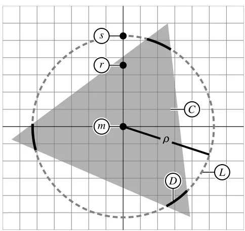
First, considerL:=H∩K, which denotes the intersection of theL1norm target hyperplane and theL2 norm target hypersphere. L essentially possesses the structure of a hypercircle, that is, all points inLlie also inH and there is a central pointm∈H and a real numberρ≥0 such that all points inLhave squared distanceρfromm. It will be shown in Appendix C thatm=λ1/n·e∈Rn andρ=λ2
2−λ 2
1/n. The intersection of the non-negative orthant with theL1norm hyperplane,C:=
Rn
≥0∩H, is a scaled canonical simplex. Its barycenter coincides with the barycentermofL. Finally, for an index setI⊆ {1, . . . ,n}letLI:={a∈L|ai=0 for alli<I}denote the subset of points from
L, where all coordinates with index not inIvanish. Its barycenter is given bymI=λ1/d·∑i
∈Iei∈Rn.
With these preparations, a simple algorithm can be proposed; it computes the sparseness-enforcing projection with respect to a constraint induced by Hoyer’s sparseness measureσ.
Theorem 2 For every x∈Rn, Algorithm 1 computes an element fromprojD(x). If r,m after line 1
Algorithm 1:Proposed algorithm for computing the sparseness-enforcing projection operator for Hoyer’s sparseness measureσ.
Input:x∈Rnandλ1,λ2∈R>0withλ2≤λ1≤ √nλ2.
Output:s∈projD(x)whereD=S(λ1,λ2) ≥0 .
// Project onto target hyperplane H and target hypercircle L.
1 r:=projH(x); 2 s∈projL(r);
// Perform alternating projections until feasible solution is found. 3 whiles<Rn
≥0do
// Project onto scaled canonical simplex C.
4 r:=projC(s);
// Project onto L keeping already vanished coordinates at zero.
5 s∈projL
I(r)whereI:={i∈ {1, . . . ,n} |ri,0};
6 end
As already pointed out, the idea of Algorithm 1 is that projections onto D can be computed by alternating projections onto the geometric structures just defined. The rigorous proof of correctness from Appendix C proceeds by showing that the set of solutions is not tampered by projection onto the intermediate structuresH,C,LandLI. Because of the non-convexity ofLandLI, the relation
between these sets and the simplexCis non-trivial and needs long arguments to be described further, see especially Lemma 26 and Corollary 27.
The projection onto the hyperplaneHis straightforward and discussed in Section C.1.1. AsLis essentially a hypersphere embedded in a subspaceHofRn, projections of points fromHontoLare achieved by shifting and scaling, see Section C.1.2. The alternating projection ontoHandLin the beginning of Algorithm 1 make the result of the projection ontoDinvariant to positive scaling and arbitrary shifting of the argument, as shown in Corollary 19. This is especially useful in practice, alleviating the need for certain pre-processing methods. The formula for projections ontoL can be generalized for projections ontoLIfor an index setI ⊆ {1, . . . ,n}, by keeping already vanished
coordinates at zero, see Section C.3.
Projections onto the simplexCare more involved and discussed at length in Section C.2. The most relevant result is that ifx∈Rn\C, then there exists a separator ˆt∈Rsuch thatp:=projC(x) = max(x−tˆ·e, 0), where the maximum is taken element-wise (Chen and Ye, 2011). In the cases considered in this paper it is always ˆt≥0 as shown in Lemma 28. This implies that all entries in x that are less than ˆt do not survive the projection, and hence theL0 pseudo-norm of xis strictly greater than that ofp. The simplex projection therefore enhances sparseness.
The separator ˆt and the number of nonzero entries in the projection ontoCcan be computed with Algorithm 2, which is an adapted version of the algorithm of Chen and Ye (2011). In line 1,Sn
denotes the symmetric group andPτdenotes the permutation matrix associated with a permutation τ∈Sn. The algorithm works by sorting its argumentxand then determining ˆtas the mean value of
Algorithm 2: Computation of information for performing projections onto C, which is a scaled canonical simplex. This is an adapted version of the algorithm of Chen and Ye (2011).
Input:x∈Rn\Candλ1∈R>0.
Output:(tˆ,d)∈R×Nsuch that projC(x) =max(x−tˆ·e, 0)andkprojC(x)k0=d.
// Sort the input vector in descending order. 1 Letτ∈Snsuch thatxτ(1)≥ ··· ≥xτ(n)andy:=Pτx∈Rn;
// Find the only feasible separator tˆ.
2 s:=0;
3 fori:=1ton−1do
4 s:=s+yi; t:= s−iλ1; 5 ift≥yi+1then return(t,i);
6 end
7 s:=s+yn; t:=s−nλ1; return(t, n);
Algorithm 3:Explicit and optimized variant of Algorithm 1.
Input:x∈Rnandλ1,λ2∈R>0withλ2≤λ1≤ √nλ2.
Output:s∈projD(x)whereD=S(λ1,λ2) ≥0 .
1 procedureproj_L(y∈Rd)
2 ρ:=λ22−λ21/d; // Compute squared radius of LI (Lemma 15).
3 ϕ:=∑di=1y2i −λ12/d; // ϕ:=ky−mIk22 (Remark 14).
4 ifϕ=0then
5 (y1, . . . , yd−1)T:=λ1/d+√ρ/√d(d−1); // y equals the barycenter of LI,
6 yd:=λ1/d−√ρ(d−1)/√d; // pick a sorted projection (Remark 18).
7 elsey:=λ1/d·e+pρ/ϕ·(y−λ1/d·e); // Pick unique projection (Lemma 17).
8 end
// Beginning of main body.
9 Letτ∈Snsuch thatxτ(1)≥ ··· ≥xτ(n)andy:=Pτx∈Rn; // Sort the input vector.
10 y:=y+1/n·(λ1−∑ni=1yi)e; // Project onto H (Lemma 13).
11 proj_L(y1, . . . ,yn); // Project in-place onto L.
// Perform alternating projections until feasible solution is found.
12 d:=n; // Store current number of relevant entries of y.
13 while(y1, . . . , yd)T <Rd≥0do
14 (tˆ,d):=proj_C(y1, . . . ,yd); // This is carried out by Algorithm 2.
15 (y1, . . . , yd)T:= (y1, . . . , yd)T−tˆ; // Project onto C (Proposition 24).
16 proj_L(y1, . . . ,yd); // Project onto LI where I={1, . . . ,d} (Lemma 30).
17 end
2.2 Optimized Variant
Because of the permutation-invariance of the sets involved in the projections, it is enough to sort the vector that is to be projected ontoDonce. This guarantees that the working vector that emerges from subsequent projections is sorted also. No additional sorting has then to be carried out when us-ing Algorithm 2 for projections ontoC. This additionally has the side effect that the non-vanishing entries of the working vector are always concentrated in its first entries. Hence all relevant infor-mation can always be stored in a small unit-stride array, to which access is more efficient than to a large sparse array. Further, the index setI of non-vanishing entries in the working vector is always of the formI={1, . . . ,d}, wheredis the number of nonzero entries.
Algorithm 3 is a variant of Algorithm 1 where these optimizations were applied, and where the explicit formulas for the intermediate projections were used. The following result, which is proved in Appendix C, states that both algorithms always compute the same result:
Theorem 3 Algorithm 1 is equivalent to Algorithm 3.
Projections ontoCincrease the amount of vanishing entries in the working vector, which is of finite dimensionn. Hence, at mostnalternating projections are carried out, and the algorithm terminates in finite time. Further, the complexity of each iteration is at most linear in theL0pseudo-norm of the working vector. The theoretic overall computational complexity is thus at most quadratic in problem dimensionalityn.
2.3 Comparison with Hoyer’s Original Algorithm
The original algorithm for the sparseness-enforcing projection operator proposed by Hoyer (2004) is hard to understand, and correctness has been proved by Theis et al. (2005) in a special case only. A simple alternative has been proposed with Algorithm 1 in this paper. Based on the symmetries induced by Hoyer’s sparseness measureσand by exploiting the projection onto a simplex, an im-proved method was given in Algorithm 3.
The improved algorithm proposed in this paper always requires at most the same number of iterations of alternating projections as the original algorithm. The original algorithm uses a pro-jection onto the non-negative orthantRn
≥0to achieve vanishing coordinates in the working vector. This operation can be written as projRn
≥0(x) =max(x, 0). In the improved algorithm, a simplex projection is used for this purpose, expressed formally as projC(x) =max(x−tˆ·e,0)with ˆt∈R
chosen accordingly. Due to the theoretical results on simplex geometry from Section C.2 and their application in Lemma 28 in Section C.3, the number ˆtis always non-negative. Therefore, at least the same amount of entries is set to zero in the simplex projection compared to the projection onto the non-negative orthant, see also Corollary 29. Hence with induction for the number of non-vanishing entries in the working vector, the number of iterations the proposed algorithm needs to terminate is bounded by the number of iterations the original method needs to terminate given the same input.
Original Algorithm Improved Algorithm
Dimensionality
N
u
m
b
e
r
o
f
It
e
ra
ti
o
n
s
2 4 6 8 10 12 14
10 10
10 10
10
101 2 3 4 5 6
Figure 1: Comparison of the number of iterations of the original algorithm for the projection ontoD with the improved version as proposed in this paper. The sparseness-enforcing projection with target sparseness 0.90 was carried out for input vectors of sparseness 0.15. The thick lines indicate the mean number of iterations required for the projection, and the thin lines indicate the minimum and maximum number of iterations, respectively. Even for input vectors with a million entries, less than 14 iterations are required to find the projection. With the improved algorithm, this reduces to at most 10 iterations.
recorded in each iteration. This was done for different dimensionalities, and for each dimensionality 1000 vectors were sampled.
Figure 1 shows statistics on the number of iterations the algorithms needed to terminate. As was already observed by Hoyer (2004), the number of required iterations grows very slowly with problem dimensionality. For n=106, only between 12 and 14 iterations were needed with the original algorithm to compute the result. With Algorithm 3, this can be improved to requiring 9 to 10 iterations, which amounts to roughly 30% less iterations. Due to the small slope in the number of required iterations, it can be conjectured that this quantity is at most logarithmic in problem dimensionalityn. If this applies, the complexity of Algorithm 3 is at most quasilinear. Because the input vector is sorted in the beginning, it is also not possible to fall below this complexity class.
The progress of working dimensionality reduction for problem dimensionalityn=1000 is de-picted in Figure 2, averaged over the 1000 input vectors from the experiment. After the first iteration, that is after projecting ontoHandL, the working dimensionality still matches the input dimension-ality. Starting with the second iteration, dimensions are discarded by projecting onto Rn
Original Algorithm Improved Algorithm
Number of Iteration
W o rk in g D im e n s io n a lit y [% ] 1 1
2 3 4 5 6 7 8 9 10
10
11 12
100
Figure 2: Comparison of the number of non-vanishing entries in the working vectors of the original algorithm and the improved algorithm during run-time. The algorithms were run with input vectors of dimensionality 1000 and initial sparseness 0.15 to compute projections with sparseness 0.90. Standard deviations were always less than 1%; they were omitted in the plot to avoid clutter. The algorithm proposed in this paper reduces dimensionality more quickly and terminates earlier than the original algorithm.
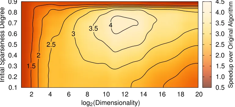
log2(Dimensionality)
In it ia l S p a rs e n e s s D e g re e S p e e d u p o ve r O ri g in a l A lg o ri th m
2 4 6 8 10 12 14 16 18 20
0.1 0.2 0.3 0.4 0.5 0.6 0.7 0.8 0.9 0.5 1.0 1.5 1.5 2.0 2.5 2.5 3.0 3.5 3.5 4.0 4.5 2 3 4
For determination of the relative speedup incorporated with both the simplex projection and the access to unit-stride arrays due to the permutation-invariance, both algorithms were implemented as C++ programs using an optimized implementation of the BLAS library for carrying out the vector operations. The employed processor was an Intel Core i7-990X. For a range of different dimension-alities, a set of vectors with varying initial sparseness were sampled. The number of the vectors for every pair of dimensionality and initial sparseness was chosen such that the processing time of the algorithms was several orders of magnitudes greater than the latency time of the operation system. Then the absolute time needed for the algorithms to compute the projections with a target sparseness of 0.90 were measured, and their ratio was taken to compute the relative speedup. The results of this experiment are depicted in Figure 3. It is evident that the maximum speedup is achieved for vectors with a dimensionality between 29 and 215, and an initial sparseness greater than 0.40. For low initial sparseness, as is achieved by randomly sampled vectors, a speedup of about 2.5 can be achieved for a broad spectrum of dimensionality between 24and 213.
The improvements to the original algorithm are thus not only theoretical, but also noticeable in practice. The speedup is especially useful when the projection is used as a neuronal transfer function in a classifier as proposed in Section 3, because then the computational complexity of the prediction of class membership of unknown samples can be reduced.
2.4 Function Definition and Differentiability
It is clear from Theorem 2 that the projection ontoDis unique almost everywhere. Therefore the setR:={x∈Rn| |projD(x)|,1}is a null set. However,R,∅as for example the projection is not unique for vectors where all entries are identical. In other words, forx:=ξe∈Rnfor someξ∈R
follows projH(x) =mand projL(m) =L. Ifn=2 a possible solution is given by(α,β)T ∈projD(x) withαandβgiven as stated in Remark 18, as in this caseαandβare positive. Additionally, another solution is given by(β,α)T ∈projD(x)which is unequal to the other solution because ofα,β. A similar argument can be used to show non-uniqueness for all n≥2. AsR is merely a small set, non-uniqueness is not an issue in practical applications.
The sparseness-enforcing projection operator that is restricted to non-negative solutions can thus be cast almost everywhere as a function
π≥0:Rn\R→D, x7→projD(x).
Exploiting reflection-invariance implies that the unrestricted variant of the projection
π:Rn\R→S(λ1,λ2), x7→s◦π
≥0(|x|),
is well-defined, wheres∈ {±1}nis given as described in Lemma 11. Note that computation ofπ≥0 is a crucial prerequisite to computation of the unrestricted variantπ. It will be used exclusively in Section 3 because non-negativity is not necessary in the application proposed there.
Ifπorπ≥0is employed in an objective function that is to be optimized, the information whether these functions are differentiable is crucial for selecting an optimization strategy. As an example, consider once more projections ontoZ:={x∈Rn| kxk0=κ}whereκ∈Nis a constant. It was already mentioned in Section 2 that the projection ontoZconsists simply of zeroing out the elements that are smallest in absolute value. Let x∈Rn be a point and let τ∈S
n be a permutation such
that xτ(1)
≥ ··· ≥ xτ(n)
. Clearly, if xτ(κ)
,
xτ(κ+1)
then projZ(x) =y where yi =xi for i∈
{τ(1), . . . ,τ(κ)} andyi=0 for i∈ {τ(κ+1), . . . ,τ(n)}. Moreover, when
xτ(κ)
,
xτ(κ+1)
there exists a neighborhoodUofxsuch that projZ(s) =∑κi=1sτ(i)eτ(i)for alls∈U. With this
closed-form expression,s7→projZ(s)is differentiable inxwith gradient∂projZ(x)/∂x=diag ∑κi=1eτ(i), that
is the identity matrix where the entries on the diagonal belonging to small absolute values ofxhave been zeroed out. If the requirement onxis not fulfilled, then a small distortion ofxis sufficient to find a point in which the projection ontoZis differentiable.
In contrast to theL0 projection, differentiability ofπandπ≥0 is non-trivial. A full-length dis-cussion is given in Appendix D, and concludes that bothπandπ≥0are differentiable almost every-where. It is more efficient when only the product of the gradient with an arbitrary vector needs to be computed, see Corollary 36. Such an expression emerges in a natural way by application of the chain rule to an objective function where the sparseness-enforcing projection is used. In practice this weaker form is thus mostly no restriction and preferable for efficiency reasons over the more general complete gradient as given in Theorem 35.
The derivative ofπ≥0is obtained by exploiting the structure of Algorithm 1. Because the projec-tion ontoDis essentially a composition of projections ontoH,C,LandLI, the overall gradient can
be computed using the chain rule. The gradients of the intermediate projections are simple expres-sions and can be combined to yield one matrix for each iteration of alternating projections. Since these iteration gradients are basically sums of dyadic products, their product with an arbitrary vector can be computed by primitive vector operations. With matrix product associativity, this process can be repeated to efficiently compute the product of the gradient ofπ≥0with an arbitrary vector. For this, it is sufficient to record some intermediate quantities during execution of Algorithm 3, which does not add any major overhead to the algorithm itself. The gradient of the unrestricted variantπ can be deduced in a straightforward way from the gradient ofπ≥0because of their close relationship. 3. Sparse Activity and Sparse Connectivity in Supervised Learning
The sparseness-enforcing projection operator can be cast almost everywhere as vector-valued func-tionπ, which is differentiable almost everywhere, see Section 2.4. This section proposes a hybrid of an auto-encoder network and a two-layer neural network, where the sparseness projection is employed as a neuronal transfer function. The proposed model is called supervised online auto-encoder (SOAE) and is intended for classification by means of a neural network that features sparse activity and sparse connectivity. Because of the analytical properties of the sparseness-enforcing projection operator, the model can be optimized end-to-end using gradient-based methods.
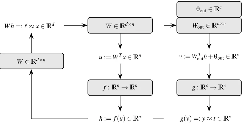
3.1 Architecture
Figure 4 depicts the data flow in the proposed model. There is one module for reconstruction ca-pabilities and one module for classification caca-pabilities. Thereconstruction module, depicted on the left of Figure 4, operates by converting an input samplex∈Rd into aninternal representation
h∈Rn, and then computing an approximation ˜x∈Rdto the original input sample. In doing so, the productu∈Rn of the input sample with amatrix of bases W ∈Rd×n is computed, and a transfer function f:Rn→Rnis applied. For sparse activity, f can be chosen to be the sparseness-enforcing
com-W∈Rd×n
θout∈Rc
Wout∈Rn×c
f:Rn→Rn g:Rc→Rc
W ∈Rd×n
W h=: ˜x≈x∈Rd
u:=WTx∈Rn v:=WoutT h+θout∈Rc
h:= f(u)∈Rn g(v) =:y≈t∈Rc
Figure 4: Architecture and data flow of supervised online auto-encoder (SOAE). The circle on the left, mapping from an input samplexto its approximation ˜xcomprises the reconstruction module. The classification module consists of the mapping fromxto the classification decisiony. The matrix of basesW shall be sparsely populated to account for the sparse connectivity property. If the transfer function f is set to the sparseness projection, the internal representationhwill be sparsely populated, fulfilling the sparse activity property.
ponent analysis (Hotelling, 1933), restricted Boltzmann machines for deep auto-encoder networks (Hinton et al., 2006) and to sparse encoding symmetric machine (Ranzato et al., 2008).
By enforcingW to be sparsely populated, the sparse connectivity property holds as well. More formally, the aim is thatσ(Wei) =σW holds for alli∈ {1, . . . ,n}, whereσW ∈(0,1)is the target
degree of connectivity sparseness andWei is thei-th column ofW. This condition was adopted
from non-negative matrix factorization with sparseness constraints (Hoyer, 2004). In the context of neural networks, the synaptic weights of individual neurons are stored in the columns of the weight matrixW. The interpretation of this formal sparseness constraint is then that each neuron is only allowed to be sparsely connected with the input layer.
The classification module is shown on the right-hand side of Figure 4. It computes a classi-fication decision y∈Rc by feedingh through a one-layer neural network. The network output y is yielded through computation of the product with a matrix of weightsWout∈Rn×c, addition of a threshold vectorθout∈Rc and application of a transfer function g:Rc→Rc. This module shares the inference of the internal representation with the reconstruction module, which can also be considered a one-layer neural network. Therefore the entire processing path fromxtoyforms a two-layer neural network (Rumelhart et al., 1986), whereW stores the synaptic weights of the hidden layer, andWoutandθoutare the parameters of the output layer.
The input samplex shall be approximated by ˜x, and the target vector for classificationt∈Rc
a differentiable similarity measuresR:Rd×Rd →R, and the approximationy≈tis assessed by
another similarity measuresC:Rc×Rc→R. For minimizing the deviation in both approximations,
the objective function
ESOAE(W,Wout,θout):= (1−α)·sR(x˜, x) +α·sC(y,t)
shall be optimized, whereα∈[0,1]controls the trade-off between reconstruction and classification capabilities. To incorporate sparse connectivity, feasible solutions are restricted to fulfillσ(Wei) =
σW for alli∈ {1, . . . ,n}. Ifα=0, then SOAE is identical to a symmetric auto-encoder network with
sparse activity and sparse connectivity. In the case ofα=1, SOAE forms a two-layer neural network for classification with a sparsely connected hidden layer and where the activity in the hidden layer is sparse. The parameterαcan also be used to blend continuously between these two extremes. Note that ˜x only depends onW but not onWout orθout, butydepends onW,Wout andθout. HenceWout andθoutare only relevant whenα>0, whereasWis essential for all choices ofα.
An appropriate choice forsR is the correlation coefficient (see for example Rodgers and
Nice-wander, 1988), because it is normed to values in the interval[−1,1], invariant to affine-linear trans-formations, and differentiable. If f is set toπ, then a model that is invariant to the concrete scaling and shifting of the occurring quantities can be yielded. This follows becauseπ is also invariant to such transformations, see Corollary 19. The similarity measure for classification capabilitiessC
is chosen to be the cross-entropy error function (Bishop, 1995), which was shown empirically by Simard et al. (2003) to induce better classification capabilities than the mean squared error func-tion. The softmax transfer function (Bishop, 1995) is used as transfer functiongof the output layer. It provides a natural pairing together with the cross-entropy error function (Dunne and Campbell, 1997) and supports multi-class classification.
3.2 Learning Algorithm
The proposed optimization algorithm for minimization of the objective functionESOAEis projected gradient descent (Bertsekas, 1999). Here, each update to the degrees of freedom is followed by ap-plication of the sparseness projection to the columns ofW to enforce sparse connectivity. There are theoretical results on the convergence of projected gradient methods when projections are carried out onto convex sets (Bertsekas, 1999), but here the target set for projection is non-convex. Never-theless, the experiments described below show that projected gradient descent is an adequate heuris-tic in the situation of the SOAE framework to tune the network parameters. For completeness, the gradients ofESOAEwith respect to the network parameters are given in Appendix E. Update steps are carried out after every presentation of a pair of an input sample and associated target vector. This online learning procedure results in faster learning and improves generalization capabilities over batch learning (Wilson and Martinez, 2003; Bottou and LeCun, 2004).
A learning set with samples from Rd and associated target vectors from {0,1}c as one-of-c -codes is input to the algorithm. The dimensionality of the internal representationnand the target degree of sparseness with respect to the connectivityσW ∈(0,1)are parameters of the algorithm.
Sparseness of connectivity increases for largerσW, as Hoyer’s sparseness measure is employed in
the definition of the set of feasible solutions.
operatorπwith respect to Hoyer’s sparseness measureσ, which can be carried out by Algorithm 3. In both cases, a target degree for sparse activity is a parameter of the learning algorithm. In case of theL0projection, this sparseness degree is denoted byκ∈ {1, . . . ,n}, and sparseness increases with smaller values of it. For the σprojection,σH ∈(0, 1)is used, where larger values indicate more
sparse activity.
Initialization of the columns ofW is achieved by selecting a random subset of the learning set, similar to the initialization of radial basis function networks (Bishop, 1995). This ensures significant activity of the hidden layer from the very start, resulting in strong gradients and therefore reducing training time. The parameters of the output layer, that isWoutandθout, are initialized by sampling from a zero-mean Gaussian distribution with a standard deviation of1/100.
In every epoch, a randomly selected subset of samples and associated target vectors from the learning set is used for stochastic gradient descent to updateW,Wout andθout. The results from Appendix E can be used to efficiently compute the gradient of the objective function. There, the gradient for the transfer function f only emerges as a product with a vector. The gradient for theL0 projection is trivial and was given as an example in Section 2.4. If fis Hoyer’s sparseness-enforcing projection operator, it is possible to exploit that only the product of the gradient with a vector is needed. In this case, it is more efficient to compute the result of the multiplication implicitly using Corollary 36 and thus avoid the computation of the entire gradient ofπ.
After every epoch, a sparseness projection is applied to the columns ofW. This guarantees that σ(Wei) =σW holds for alli∈ {1, . . . ,n}, and therefore the sparse connectivity property is fulfilled.
The trade-off variableαwhich controls the weight of the reconstruction and the classification term is adjusted according toα(ν):=1−exp(−ν/100), whereν∈Ndenotes the number of the current epoch. Thus α starts at zero, increases slowly and asymptotically reaches one. The emphasis at the beginning of the optimization is thus on reconstruction capabilities. Subsequently, classification capabilities are incorporated slowly, and in the final phase of training classification capabilities ex-clusively are optimized. This continuous variant of unsupervised pre-training (Hinton et al., 2006) leads to parameters in the vicinity of a good minimizer for classification capabilities before classi-fication is preferred over reconstruction through the trade-off parameterα. Compared to the choice α≡1 this strategy helps to stabilize the trajectory in parameter space and makes the objective function values settle down more quickly, such that the termination criterion is satisfied earlier.
3.3 Description of Experiments
To assess the classification capabilities and the impact of sparse activity and sparse connectivity, the MNIST database of handwritten digits (LeCun and Cortes, 1998) was employed. It is a popular benchmark data set for classification algorithms, and numerous results with respect to this data set are reported in the literature. The database consists of 70 000 samples, divided into a learning set of 60 000 samples and an evaluation set of 10 000 samples. Each sample represents a digit of size 28×28 pixels and has a class label from{0, . . . ,9}associated with it. Therefore the input and output dimensionalities ared:=282=784 andc:=10, respectively. The classification error is given in percent of all 10 000 evaluation samples, hence 0.01% corresponds to a single misclassified digit.
directions by one pixel, yielding 540 000 samples for learning in total. The evaluation set was left unchanged to yield results that can be compared to the literature. As noted by Hinton et al. (2006), the learning problem is no more permutation-invariant due to the jittering, as information on the neighborhood of the pixels is implicitly incorporated in the learning set.
However, classification results improve dramatically when such prior knowledge is used. This was demonstrated by Schölkopf (1997) using the virtual support vector method, which improved a support vector machine with polynomial kernel of degree five from an error of 1.4% to 1.0% by jittering the support vectors by one pixel in four principal directions. This result was extended by DeCoste and Schölkopf (2002), where a support vector machine with a polynomial kernel of degree nine was improved from an error of 1.22% to 0.68% by jittering in all possible eight directions. Further improvements can be achieved by generating artificial training samples using elastic distor-tions (Simard et al., 2003). This reduced the error of a two-layer neural network with 800 hidden units to 0.7%, compared to the 1.1% error yielded when training on samples created by affine dis-tortions. Very big and very deep neural networks possess a large number of adaptable weights. In conjunction with elastic and affine distortions such neural networks can yield errors as low as 0.35% (Cire¸san et al., 2010). The current record error of 0.23% is held by an approach that combines dis-torted samples with a committee of convolutional neural networks (Cire¸san et al., 2012). This is an architecture that has been optimized exclusively for input data that represents images, that is where the neighborhood of the pixels is hard-wired in the classifier. To allow for a plain evaluation that does not depend on additional parameters for creating artificial samples, the jittered learning set with 540 000 samples is used throughout this paper.
The experimental methodology was as follows. The number of hidden units was chosen to be n:=1000 in all experiments that are described below. This is an increased number compared to the 800 hidden units employed by Simard et al. (2003), but promises to yield better results when an adequate number of learning samples is used. As all tested learning algorithms are essentially gradient descent methods, an initial step size had to be chosen. For each candidate step size, five runs of a two-fold cross validation were carried out on the learning set. Then, for each step size the median of the ten resulting classification errors was computed. The winning step size was then determined to be the one that achieved a minimum median of classification errors.
In every epoch, 21 600 samples were randomly chosen from the learning set and presented to the network. This number of samples was chosen as it is 1/25-th of the jittered learning set. The step size was multiplicatively annealed using a factor of 0.999 after every epoch. Optimization was terminated once the relative change in the objective function became very small and no more significant progress on the learning set could be observed. The resulting classifiers were then applied to the evaluation set, and misclassifications were counted.
3.4 Experimental Results
Two variants of the supervised online auto-encoder architecture as proposed in this section were trained on the augmented learning set. In both variants, the target degree of sparse connectivity was set toσW :=0.75. This choice was made because 96% of all samples in the learning set possess
a sparseness which is less than 0.75. Therefore, the resulting bases are forced to be truly sparsely connected compared to the sparseness of the digits.
to Hoyer’s sparseness measureσwere chosen from the interval[0.20,0.95]in steps of size 0.05. This variant was then trained on the jittered learning set using the method described in Section 3.2. For every value ofσH, the resulting sparseness of activity was measured after training using the
L0 pseudo-norm. For this, each sample of the learning set was presented to the networks, and the number of active units in the hidden layer was counted. Figure 5 shows the resulting mean value and standard deviation of sparse activity. IfσH=0.20 is chosen, then in the mean about 800 of the total
1000 hidden units are active upon presentation of a sample from the learning set. ForσH=0.80 only
one hundred units are active at any one time, and forσH=0.95 there are only eleven active units.
The standard deviation of the activity decreases when sparseness increases, hence the mapping from σHto the resulting number of active units becomes more accurate.
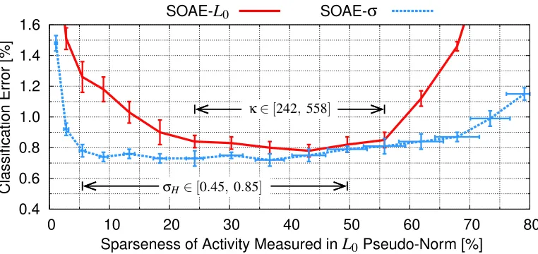
The second variant, denoted SOAE-L0, differs from SOAE-σin that the projection with respect to theL0pseudo-norm as transfer function f was used. The target sparseness of activity is given by a parameterκ∈ {1, . . . ,n}, which controls the exact number of units that are allowed to be active at any one time. For the experiments, the values forκwere chosen to match the mean activities from the SOAE-σexperiments. This way the results of both variants can be compared based on a unified value of activity sparseness. The results are depicted in Figure 6. Usage of theσprojection consequently outperforms theL0projection for all sparseness degrees. Even for high sparseness of activity, that is when only about ten percent of the units are allowed to be active at any one time, good classification capabilities can be obtained with SOAE-σ. For κ∈[242, 558], the classifica-tion results of SOAE-L0reach an optimum. SOAE-σis more robust, as classification capabilities first begin to collapse when sparseness is below 5%, whereas SOAE-L0 starts to degenerate when sparseness falls below 20%. For σH∈[0.45, 0.85], roughly translating to between 5% and 50%
activity, about equal classification performance is achieved using SOAE-σ.
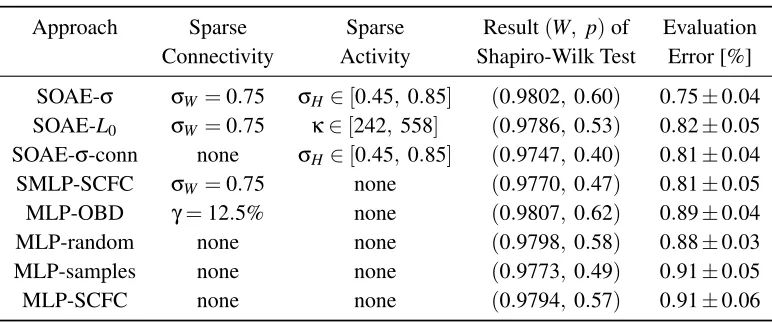
It can thus be concluded that using the sparseness-enforcing projection operator as described in this paper yields better results than when the simpleL0projection is used to achieve sparse activity. To assess the benefit more precisely and to investigate the effect of individual factors, several com-parative experiments have been carried out. A summary of these experiments and their outcome is given in Table 1. The variants SOAE-σand SOAE-L0 denote the entirety of the respective exper-iments where sparseness of activity lies in the intervals described above, that isσH∈[0.45,0.85]
andκ∈[242,558], respectively. Using these intervals, SOAE-σand SOAE-L0achieved a median error of 0.75% and 0.82% on the evaluation set, respectively. Variant SOAE-σ-conn is essentially equal to SOAE-σ, except for sparse connectivity not being incorporated. Sparseness of activity here was also chosen to beσH ∈[0.45,0.85], which resulted in about equal classification results over
the entire range. Dropping of sparse connectivity increases misclassifications, for the median error of SOAE-σ-conn is 0.81% and thereby greater than the median error of SOAE-σ.
The other five approaches included in the comparison are multi-layer perceptrons (MLPs) with the same topology and dynamics as the classification module of supervised online auto-encoder, with two exceptions. First, the transfer function of the hidden layerfwas set to a hyperbolic tangent, thus not including explicit sparse activity. Second, in all but one experiment sparse connectivity was either not incorporated, or achieved through other means than by performing aσprojection after each learning epoch. Besides the variation in sparseness of connectivity, the experiments differ in the initialization of the network parameters.
Sparseness Degree with Respect to Sparseness Measureσ L0
P
s
e
u
d
o
-N
o
rm
[%
]
0 20 40 60 80 100
0.2 0.3 0.4 0.5 0.6 0.7 0.8 0.9 1.0
Figure 5: Resulting amount of nonzero entries in an internal representation h with 1000 entries, depending on the target degree of sparseness for activity σH with respect to Hoyer’s
sparseness measure σ. For low values of σH, about 80% of the entries are nonzero,
whereas for very high sparseness degrees only 1% of the entries do not vanish. The error bars indicate±one standard deviation distance from the mean value. Standard deviation shrinks with increasing sparseness degree, making the mapping more accurate.
SOAE-L0 SOAE-σ
Sparseness of Activity Measured inL0Pseudo-Norm [%]
C
la
s
s
ifi
c
a
ti
o
n
E
rr
o
r
[%
]
κ∈[242,558]
σH∈[0.45,0.85]
0 10 20 30 40 50 60 70 80
0.4 0.6 0.8 1.0 1.2 1.4 1.6
Approach Sparse Sparse Result(W, p)of Evaluation Connectivity Activity Shapiro-Wilk Test Error [%]
SOAE-σ σW =0.75 σH∈[0.45,0.85] (0.9802,0.60) 0.75±0.04
SOAE-L0 σW =0.75 κ∈[242, 558] (0.9786,0.53) 0.82±0.05
SOAE-σ-conn none σH∈[0.45,0.85] (0.9747,0.40) 0.81±0.04
SMLP-SCFC σW =0.75 none (0.9770,0.47) 0.81±0.05
MLP-OBD γ=12.5% none (0.9807,0.62) 0.89±0.04 MLP-random none none (0.9798,0.58) 0.88±0.03 MLP-samples none none (0.9773,0.49) 0.91±0.05 MLP-SCFC none none (0.9794,0.57) 0.91±0.06
Table 1: Overview of comparative experiments. The second and third columns indicate whether sparse connectivity or sparse activity was incorporated, respectively. The fourth column reports the result of a statistical test for normality, which is interpreted in Section 3.5. The final column gives the median±one standard deviation of the achieved classification error on the MNIST evaluation set. The results for each experiment were trimmed to gain a sample of size 47, allowing for statistical robust estimates.
where 15% of the original data were trimmed away. This procedure was also applied to the results of SOAE-σ, SOAE-σ-conn, and SOAE-L0, to obtain a total of eight random samples of equal size for comparison with another.
The most basic variant, denoted the baseline in this discussion, is MLP-random, where all net-work parameters were initialized randomly. This achieved a median error of 0.88% on the evalua-tion set, being considerably worse than SOAE-σ. For variant MLP-samples, the hidden layer was initialized by replication ofn randomly chosen samples from the learning set. This did decrease the overall learning time. However, the median classification error was slightly worse with 0.91% compared to MLP-random.
For variant MLP-SCFC, the network parameters were initialized in an unsupervised manner us-ing the sparse codus-ing for fast classification (SCFC) algorithm (Thom et al., 2011a). This method is a precursor to the SOAE proposed in this paper. It also features sparse connectivity and sparse activity but differs in some essential parts. First, sparseness of activity is achieved through a latent variable that stores the optimal sparse code words of all samples simultaneously. Using this matrix of code words, the activity of individual units was enforced to be sparse over time on the entire learning set. SOAE achieves sparseness over space, as for each sample only a pre-defined fraction of units is allowed to be active at any one time. A second difference is that sparse activity is achieved only indirectly by approximation of the latent matrix of code words with a feed-forward represen-tation. With SOAE, sparseness of activity is guaranteed by construction. MLP-SCFC achieved a median classification error of 0.91% on the MNIST evaluation set, rendering it slightly worse than MLP-random and equivalent to MLP-samples.
every learning epoch. Hence the sparseness gained from unsupervised initialization was retained. MLP-SCFC features sparse connectivity only after initialization, but loses this property when train-ing proceeds. With this slight modification, the median error of SMLP-SCFC decreases to 0.81%, which is significantly better than the baseline result.
The effect of better generalization due to sparse connectivity has also been observed by LeCun et al. (1990) in the context of convolutional neural networks. It can be explained by the bias-variance decomposition of the generalization error (Geman et al., 1992). When the effective number of the degrees of freedom is constrained, overfitting will be less likely and hence classifiers produce better results on average. The same argument can be applied to SOAE-σ, where additional sparse activity further improves classification results.
The last variant is called MLP-OBD. Here, the optimal brain damage (OBD) algorithm (LeCun et al., 1990) was used to prune synaptic connections in the hidden layer that are irrelevant for the computation of the classification decision of the network. The parameters of the network were first initialized randomly and then optimized on the learning set. Then the impact for each synaptic connection on the objective function was estimated using the Taylor series of the objective function, where a diagonal approximation of the Hessian was employed and terms of cubic or higher order were neglected. Using this information, the number of connections was halved by setting the weight of connections with low impact to zero. The network was then retrained with weights of removed connections kept at zero. This procedure was repeated until a target percentageγof active synaptic connections in the hidden layer was achieved. For the results reported here,γ=12.5% was chosen as this reflects the sparse connectivityσW=0.75 of the other approaches best. MLP-OBD achieved
a median classification error of 0.89%, which is comparable to the baseline result.
3.5 Statistical Analysis and Conclusions
A statistical analysis was carried out to assess the significance of the differences in the performance of the eight algorithms. The procedure follows the proposals of Pizarro et al. (2002) and Demšar (2006) for hypothesis testing, and is concluded by effect size estimation as proposed by Grissom (1994) and Acion et al. (2006). For each algorithm, a sample of size 47 was available, allowing for robust analysis results.
First, all results were tested for normality using the test developed by Shapiro and Wilk (1965). The resulting test statisticsW andp-values are given in Table 1. As allp-values are large, it cannot be rejected that the samples came from normally distributed populations. Thus normality is assumed in the remainder of this discussion. Next, the test proposed by Levene (1960) was applied to deter-mine whether equality of variances of the groups holds. This resulted in a test statisticF=2.7979 with 7 and 368 degrees of freedom, and therefore a p-value of 0.0075. Hence the hypothesis that all group variances are equal can be rejected with very high significance. Consequently, parametric omnibus and post-hoc tests cannot be applied, as they require the groups to have equal variance.
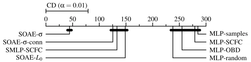
0 50 100 150 200 250 300 CD (α=0.01)
SOAE-σ MLP-samples
SOAE-σ-conn MLP-SCFC
SMLP-SCFC MLP-OBD
SOAE-L0 MLP-random
Figure 7: Diagram for multiple comparison of algorithms following Demšar (2006). For each algo-rithm, the mean rank was computed during the Kruskal-Wallis test. Then, a critical dif-ference (CD) was computed at theα=0.01 significance level. Two algorithms produce classification results that are statistically not equal if the difference between their mean ranks is greater than the critical difference. This induced three groups of algorithms that produced statistically equivalent results, which are marked with black bars.
test (Hochberg and Tamhane, 1987). Note that this approach is nevertheless similar to the post-hoc procedure proposed by Demšar (2006) for paired observations, such that the diagrams proposed there can be adapted to the case for unpaired observations. The result is depicted in Figure 7, where the critical difference for statistical significance at theα=0.01 level is given. This test induces a highly significant partitioning of the eight algorithms, namely three groupsA,BandCgiven by
A:={SOAE-σ}, B:={SOAE-σ-conn, SOAE-L0, SMLP-SCFC}, andC:={MLP-OBD,MLP-random, MLP-samples, MLP-SCFC}.
This partition in turn induces an equivalence relation. Statistical equivalence is hence unambiguous and well-defined atα=0.01. Moreover, thep-value for this partition is 0.007. If the significance levelαwould have been set lower than this, then groupsAandBwould blend together.
To assess the benefit when an algorithm from one group is chosen over an algorithm from another group, the probability of superior experiment outcome was estimated (Grissom, 1994; Acion et al., 2006). For this, the classification errors were pooled with respect to membership in the three groups. It was then tested whether these pooled results still come from normal distributions. As group A is a singleton, this is trivially fulfilled with the result from Table 1. For group B, the Shapiro-Wilk test statistic wasW =0.9845 and the p-value was 0.11. GroupC achieved a test statistic ofW=0.9882 and ap-value of 0.12. If a standard significance level ofα=0.01 is chosen, thenBandCcan be assumed to be normally distributed also.
LetEGbe the random variable modeling the classification results of the algorithms from group
G∈ {A,B,C}. It is assumed thatEGis normally distributed with unknown mean and unknown
can be estimated by 0.99. Therefore, the effect of choosing SOAE-σover any of the seven other algorithms is dramatic (Grissom, 1994).
These results can be interpreted as follows. When neither sparse activity nor sparse connectivity is incorporated, then the worst classification results are obtained regardless of the initialization of the network parameters. The exception is MLP-OBD which incorporates sparse connectivity, although, as its name says, in a destructive way. Once a synaptic connection has been removed, it cannot be recovered, as the measure for relevance of LeCun et al. (1990) vanishes for synaptic connections of zero strength. The statistics for SMLP-SCFC shows that when sparse connectivity is obtained using the sparseness-enforcing projection operator, then superior results can be achieved. Because of the nature of projected gradient descent, it is possible here to restore deleted connections if it helps to decrease the classification error during learning. For SOAE-σ-conn only sparse activity was used, and classification results were statistically equivalent to SMLP-SCFC.
Therefore, using either sparse activity or sparse connectivity improves classification capabilities. When both are used, then results improve even more as variant SOAE-σ shows. This does not hold for SOAE-L0 however, where the L0 projection was used as transfer function. As Hoyer’s sparseness measureσand the according projection possess desirable analytical properties, they can be considered smooth approximations to theL0pseudo-norm. It is this smoothness which seems to produce this benefit in practice.
4. Related Work
This section reviews work related with the contents of this paper. First, the theoretical foundations of the sparseness-enforcing projection operator are discussed. Next, its application as neuronal trans-fer function to achieve sparse activity in a classification scenario is put in context with alternative approaches, and possible advantages of sparse connectivity are described.
4.1 Sparseness-Enforcing Projection Operator
The first major part of this paper dealt with improvements to the work of Hoyer (2004) and Theis et al. (2005). Here, an algorithm for the sparseness-enforcing projection with respect to Hoyer’s sparseness measureσ was proposed. The technical proof of correctness is given in Appendix C. The set that should be projected onto is an intersection of a simplexCand a hypercircleL, which is a hypersphere lying in a hyperplane. The overall procedure can be described as performing alternating projections ontoC and certain subsets of L. This approach is common for handling projections onto intersections of individual sets. For example, von Neumann (1950) proposed essentially the same idea when the investigated sets are closed subspaces, and has shown that this converges to a solution. A similar approach can be carried out for intersections of closed, convex cones (Dykstra, 1983), which can be generalized to translated cones that can be used to approximate any convex set (Dykstra and Boyle, 1987). For these alternating methods, it is only necessary to know how projections onto individual members of the intersection can be achieved.
degree of sparseness can be obtained. This is because when the targetL1 norm λ1 is fixed, the sparseness measure σdecreases whenever the targetL2 norm decreases. In geometric terms, the method proposed in this paper performs a projection from within a circle onto its boundary to increase the sparseness of the working vector. This argument is given in more detail in Figure 11 and the proof of Lemma 28(f).
The second drawback of the general methods for projecting onto intersections is that a solution is only achieved asymptotically, even when the convexity requirements are fulfilled. Due to the special structure ofCandL, the number of alternating projections that have to be carried out to find a solution using Algorithm 3 is bounded from above by the problem dimensionality. Thus an exact projection is always found in finite time. Furthermore, the solution is guaranteed to be found in time that is at most quadratic in problem dimensionality.
A crucial point is the computation of the projection ontoC and certain subsets ofL. Due to the nature of theL2 norm, the latter is straightforward. For the former, efficient algorithms have been proposed recently (Duchi et al., 2008; Chen and Ye, 2011). When only independent solutions are required, the projection of a pointxonto a scaled canonical simplex ofL1normλ1can also be carried out in linear time (Liu and Ye, 2009), without having to sort the vector that is to be projected. This can be achieved by showing that the separator ˆtfor performing the simplex projection is the unique zero of the monotonically decreasing functiont7→ kmax(|x| −t·e, 0)k1−λ1. The zero of this function can be found efficiently using the bisection method, and exploiting the special structure of the occurring expressions (Liu and Ye, 2009).
In the context of this paper an explicit closed-form expression for ˆt is preferable as it permits additional insight into the properties of the projected point. The major part in proving the correctness of Algorithm 1 is the interconnection between C and L, that is that the final solution has zero entries at the according positions in the working vector and thus a chain monotonically decreasing inL0pseudo-norm is achieved. This result is established through Lemma 26, which characterizes projections onto certain faces of a simplex, Corollary 27 and their application in Lemma 28.
Analysis of the theoretical properties of the sparseness-enforcing projection is concluded with its differentiability in Appendix D. The idea is to exploit the finiteness of the projection sequence and to apply the chain rule of differential calculus. It is necessary to show that the projection chain is robust in a neighborhood of the argument. This reduces analysis to individual projection steps which have already been studied in the literature. For example, the projection onto a closed, convex set is guaranteed to be differentiable almost everywhere (Hiriart-Urruty, 1982). Here non-convexity ofLis not an issue, as the only critical point is its barycenter. For the simplexC, a characterization of critical points is given with Lemma 32 and Lemma 33, and it is shown that the expression for the projection ontoC is invariant to local changes. An explicit expression for construction of the gradient of the sparseness-enforcing projection operator is given in Theorem 35. In Corollary 36 it is shown that the computation of the product of the gradient with an arbitrary vector can be achieved efficiently by exploiting sparseness and the special structure of the gradient.
Closely related with the work of this paper is the generalization of Hoyer’s sparseness measure by Theis and Tanaka (2006). Here, theL1norm constraint is replaced with a generalizedLp
pseudo-norm constraint, such that the sparseness measure becomesσp(x):=kxkp/kxk2. Forp=1, Hoyer’s
sparseness measure up to a constant normalization is obtained. When pconverges decreasingly to zero, thenσp(x)pconverges point-wise to theL0pseudo-norm. Hence for small values ofpa more
natural sparseness measure is obtained. Theis and Tanaka (2006) also proposed an extension of Hoyer’s projection algorithm. It is essentially von Neumann’s alternating projection method, where closed subspaces have been replaced by "spheres" that are induced byLp pseudo-norms. Note that
these sets are non-convex whenp<1, such that convergence is not guaranteed. Further, no closed-form solution for the projection onto an "Lp-sphere" is known forp<{1,2,∞}, such that numerical
methods have to be employed.
A problem where similar projections are employed is to minimize a convex function subject to group sparseness (see for example Friedman et al., 2010). In this context, mixed norm balls are of particular interest (Sra, 2012). For a matrixX ∈Rn×g, the mixed L
p,q norm is defined as theLp
norm of theLqnorms of the columns ofX, that iskXkp,q:=
kX e1kq, . . . , kX egkq T
p. Here,
X can be interpreted to be a data point with entries partitioned intoggroups. Whenp=1, then the projection onto a simplex can be generalized directly forq=2 (van den Berg et al., 2008) and for q=∞(Quattoni et al., 2009). The case when p=1 andq≥1 is more difficult, but can be solved as well (Liu and Ye, 2010; Sra, 2012).
The last problem discussed here is the elastic net criterion (Zou and Hastie, 2005), which is a constraint on the sum of an L1 norm and an L2 norm. The feasible set can be written as the convex set N:={s∈Rn|λ1ksk1+λ2ksk22≤1}, where λ1,λ2≥0 control the shape ofN. Note that inNonly the sum of two norms is considered, whereas the non-convex setS(λ1,λ2)consists of the intersection of two different constraints. Therefore, the elastic net induces a different notion of sparseness than Hoyer’s sparseness measure σdoes. As is the case for mixed norm balls, the projection onto a simplex can be generalized to achieve projections ontoN(Mairal et al., 2010).
4.2 Supervised Online Auto-Encoder
The sparseness-enforcing projection operatorπwith respect to Hoyer’s sparseness measureσand the projection onto anL0pseudo-norm constraint are differentiable almost everywhere. Thus they are suitable for gradient-based optimization algorithms. In Section 3, they were used as transfer functions in a hybrid of an auto-encoder network and a two-layer neural network to infer a sparse internal representation. This representation was subsequently employed to approximate the input sample and to compute a classification decision. In addition, the matrix of bases which was used to compute the internal representation was enforced to be sparsely populated by application of the sparseness projection after each learning epoch. Hence the supervised online auto-encoder proposed in this paper features both sparse activity and sparse connectivity.
A purely generative model that also possesses these two key properties is non-negative matrix factorization with sparseness constraints (Hoyer, 2004). This is an extension to plain non-negative matrix factorization (Paatero and Tapper, 1994) which was shown to achieve sparse connectivity on certain data sets (Lee and Seung, 1999). However, there are data sets on which this does not work (Li et al., 2001; Hoyer, 2004). Although Hoyer’s model makes sparseness easily controllable by explicit constraints, it is not inherently suited to classification tasks. An extension intended to incorporate class membership information to increase discriminative capabilities was proposed by Heiler and Schnörr (2006). In their approach, an additional constraint was added ensuring that every internal representation is close to the mean of all internal representations that belong to the same class. In other words, the method can be interpreted as supervised clustering, with the number of clusters equal to the number of classes. However, there is no guarantee that a distribution of internal representations exists such that both the reproduction error is minimized and the internal representations can be arranged in such a pattern. Unfortunately, Heiler and Schnörr (2006) used only a subset of a small data set for handwritten digit recognition to evaluate their approach.
A precursor to the supervised online auto-encoder was proposed by Thom et al. (2011a). There, inference of sparse internal representations was achieved by fitting a one-layer neural network to approximate a latent variable of optimal sparse representations. The transfer function used for this approximation was a hyperbolic tangent raised to an odd power greater or equal to three. This resulted in a depression of activities with small magnitude, favoring sparseness of the result. Similar techniques to achieve a shrinkage-like effect for increasing sparseness of activity in a neural network were used by Gregor and LeCun (2010) and Glorot et al. (2011). Information processing is here purely local, that is a scalar function is evaluated entrywise on a vector, and thus no information is interchanged among individual entries.
The use of non-local shrinkage to reduce Gaussian noise in sparse coding has already been de-scribed by Hyvärinen et al. (1999). Here, a maximum likelihood estimate with only weak assump-tions yields a shrinkage operation, which can be conceived as projection onto a scaled canonical simplex. In the use case of object recognition, a hard shrinkage was also employed to de-noise filter responses (Mutch and Lowe, 2006). Whenever a best approximation from a permutation-invariant set is used, a shrinkage-like operation must be employed. Using a projection operator as neural transfer function is hence a natural extension of these ideas. When the projection is suf-ficiently smooth, the entire model can be tuned end-to-end using gradient methods to achieve an auto-encoder or a classifier.