Particle Gibbs with Ancestor Sampling
Fredrik Lindsten [email protected]
Department of Engineering University of Cambridge Cambridge, CB2 1PZ, UK, and
Division of Automatic Control Link¨oping University
Link¨oping, 581 83, Sweden
Michael I. Jordan [email protected]
Computer Science Division and Department of Statistics University of California
Berkeley, CA 94720, USA
Thomas B. Sch¨on [email protected]
Department of Information Technology Uppsala University
Uppsala, 751 05, Sweden
Editor:Yee Whye Teh
Abstract
Particle Markov chain Monte Carlo (PMCMC) is a systematic way of combining the two main tools used for Monte Carlo statistical inference: sequential Monte Carlo (SMC) and Markov chain Monte Carlo (MCMC). We present a new PMCMC algorithm that we refer to as particle Gibbs with ancestor sampling (PGAS). PGAS provides the data analyst with an off-the-shelf class of Markov kernels that can be used to simulate, for instance, the typically high-dimensional and highly autocorrelated state trajectory in a state-space model. The ancestor sampling procedure enables fast mixing of the PGAS kernel even when using seemingly few particles in the underlying SMC sampler. This is important as it can significantly reduce the computational burden that is typically associated with using SMC. PGAS is conceptually similar to the existing PG with backward simulation
(PGBS) procedure. Instead of using separate forward and backward sweeps as in PGBS, however, we achieve the same effect in a single forward sweep. This makes PGAS well suited for addressing inference problems not only in state-space models, but also in models with more complex dependencies, such as non-Markovian, Bayesian nonparametric, and general probabilistic graphical models.
Keywords: particle Markov chain Monte Carlo, sequential Monte Carlo, Bayesian infer-ence, non-Markovian models, state-space models
1. Introduction
Jo-hansen, 2011; Del Moral et al., 2006) and Markov chain Monte Carlo (MCMC, see, e.g., Robert and Casella, 2004; Liu, 2001) methods in particular have found application to a wide range of data analysis problems involving complex, high-dimensional models. These include state-space models (SSMs) which are used in the context of time series and dynamical sys-tems modeling in a wide range of scientific fields. The strong assumptions of linearity and Gaussianity that were originally invoked for SSMs have indeed been weakened by decades of research on SMC and MCMC. These methods have not, however, led to a substan-tial weakening of a further strong assumption, that of Markovianity. It remains a major challenge to develop efficient inference algorithms for models containing a latent stochastic process which, in contrast with the state process in an SSM, is Markovian. Such non-Markovian latent variable models arise in various settings, either from direct modeling or via a transformation or marginalization of an SSM. We discuss this further in Section 6; see also Lindsten and Sch¨on (2013, Section 4).
In this paper we present a new tool in the family of Monte Carlo methods which is par-ticularly useful for inference in SSMs and, importantly, in non-Markovian latent variable models. However, the proposed method is by no means limited to these model classes. We work within the framework of particle MCMC (PMCMC, Andrieu et al., 2010) which is a systematic way of combining SMC and MCMC, exploiting the strengths of both tech-niques. More specifically, PMCMC samplers make use of SMC to construct efficient, high-dimensional MCMC kernels. These kernels can then be used as off-the-shelf components in MCMC algorithms and other inference strategies relying on Markov kernels. PMCMC has in a relatively short period of time found many applications in areas such as hydrology (Vrugt et al., 2013), finance (Pitt et al., 2012), systems biology (Golightly and Wilkinson, 2011), and epidemiology (Rasmussen et al., 2011), to mention a few.
Our method builds on the particle Gibbs (PG) sampler proposed by Andrieu et al. (2010). In PG, the aforementioned Markov kernel is constructed by running an SMC sampler in which one particle trajectory is set deterministically to a reference trajectory that is specified a priori. After a complete run of the SMC algorithm, a new trajectory is obtained by selecting one of the particle trajectories with probabilities given by their importance weights. The effect of the reference trajectory is that the resulting Markov kernel leaves its target distribution invariant, regardless of the number of particles used in the underlying SMC algorithm.
However, PG suffers from a serious drawback, which is that the mixing of the Markov kernel can be very poor when there is path degeneracy in the underlying SMC sampler (Lind-sten and Sch¨on, 2013; Chopin and Singh, 2014). Unfortunately, path degeneracy is in-evitable for high-dimensional problems, which significantly reduces the applicability of PG. This problem has been addressed in the generic setting of SSMs by adding a backward sim-ulation step to the PG sampler, yielding a method denoted asPG with backward simulation (PGBS, Whiteley, 2010; Whiteley et al., 2010; Lindsten and Sch¨on, 2012). It has been found that this considerably improves mixing, making the method much more robust to a small number of particles as well as growth in the size of the data (Lindsten and Sch¨on, 2013; Chopin and Singh, 2014; Whiteley et al., 2010; Lindsten and Sch¨on, 2012).
during the backward simulation pass (see Section 6.2 for details). The method proposed in this paper, which we refer to as particle Gibbs with ancestor sampling (PGAS), is geared toward this issue. PGAS alleviates the problem with path degeneracy by modifying the original PG kernel with a so-called ancestor sampling (AS) step, thereby achieving the same effect as backward sampling, but without an explicit backward pass.
After giving some background on SMC in Section 2, the PGAS Markov kernel is con-structed and analyzed theoretically in Sections 3 and 4, respectively. This extends the preliminary work that we have previously published (Lindsten et al., 2012) with a more straightforward construction, a more complete proof of invariance, and a new uniform er-godicity result. We then show specifically how PGAS can be used for inference and learning of SSMs and of non-Markovian latent variable models in Sections 5 and 6, respectively. As part of our development, we also propose a truncation strategy specifically for non-Markovian models. This is a generic method that is also applicable to PGBS, but, as we show in a simulation study in Section 7, the effect of the truncation error is much less severe for PGAS than for PGBS. Indeed, we obtain up to an order-of-magnitude increase in accuracy in using PGAS when compared to PGBS in this study. We also evaluate PGAS on a stochastic volatility SSM and on an epidemiological model. Finally, in Section 8 we conclude and point out possible directions for future work.
2. Sequential Monte Carlo
Letγθ,t(x1:t), fort= 1, . . . , T, be a sequence of unnormalized densities1 on the measurable
space (Xt,Xt), parameterized by θ ∈ Θ. Let ¯γ
θ,t(x1:t) be the corresponding normalized
probability densities:
¯
γθ,t(x1:t) =
γθ,t(x1:t)
Zθ,t
,
where Zθ,t =
R
γθ,t(x1:t)dx1:t and where it is assumed thatZθ,t >0,∀θ∈Θ. For instance,
in the (important) special case of an SSM we have ¯γθ,t(x1:t) = pθ(x1:t | y1:t), γθ,t(x1:t) =
pθ(x1:t, y1:t), andZθ,t =pθ(y1:t). We discuss this special case in more detail in Section 5.
To make inference about the latent variables x1:T, as well as to enable learning of
the model parameter θ, a useful approach is to construct a Monte Carlo algorithm to draw samples from ¯γθ,T(x1:T). The sequential nature of the problem suggests the use of
SMC methods; in particular, particle filters (PFs); see, e.g., Doucet and Johansen (2011); Del Moral et al. (2006); Pitt and Shephard (1999).
We start by reviewing a standard SMC sampler, which will be used to construct the PGAS algorithm in the consecutive section. We will refer to the index variable t as time, but in general it might not have any temporal meaning. Let{xi1:t−1, wit−1}N
i=1be a weighted
particle system targeting ¯γθ,t−1(x1:t−1). That is, the weighted particles define an empirical
point-mass approximation of the target distribution given by
b
γθ,tN−1(dx1:t−1) = N
X
i=1
wti−1
P
lwlt−1
δxi
1:t−1(dx1:t−1).
This particle system is propagated to time tby sampling {ait, xit}N
i=1 independently,
condi-tionally on the particles generated up to time t−1, from a proposal kernel,
Mθ,t(at, xt) =
wat
t−1
P
lwlt−1
rθ,t(xt|xa1:tt−1). (1)
Note thatMθ,t depends on the complete particle system up to timet−1,{xi1:t−1, wti−1}Ni=1,
but for notational convenience we shall not make that dependence explicit. Here,ait is the index of the ancestor particle of xit. In this formulation, the resampling step is implicit and corresponds to sampling these ancestor indices. When we write xi1:t we refer to the ancestral path of particlexit. That is, the particle trajectory is defined recursively as
xi1:t= (xait
1:t−1, xit).
Once we have generatedN ancestor indices and particles from the proposal kernel (1), the particles are weighted according to wti =Wθ,t(xi1:t) where the weight function is given by
Wθ,t(x1:t) =
γθ,t(x1:t)
γθ,t−1(x1:t−1)rθ,t(xt|x1:t−1)
, (2)
for t≥ 2. The procedure is initialized by sampling from a proposal density xi1 ∼ rθ,1(x1)
and assigning importance weights w1i = Wθ,1(xi1) with Wθ,1(x1) = γθ,1(x1)/rθ,1(x1). The
SMC sampler is summarized in Algorithm 1.
Algorithm 1 Sequential Monte Carlo (each step is for i= 1, . . . , N) 1: Draw xi1 ∼rθ,1(x1).
2: Setwi1=Wθ,1(xi1).
3: fort= 2 toT do
4: Draw {ait, xit} ∼Mθ,t(at, xt).
5: Setxi1:t= (xa
i t
1:t−1, xit).
6: Setwti=Wθ,t(xi1:t).
7: end for
It is interesting to note that the joint law of all the random variables generated by Algorithm 1 can be written down explicitly. Let
xt={x1t, . . . , xNt } and at={a1t, . . . , aNt },
refer to all the particles and ancestor indices, respectively, generated at time t of the algorithm. It follows that the SMC sampler generates a collection of random variables
{x1:T,a2:T} ∈XN T× {1, . . . , N}N(T−1). Furthermore,{ait, xit}Ni=1 are drawn independently
(conditionally on the particle system generated up to timet−1) from the proposal kernel Mθ,t, and similarly at timet= 1. Hence, the joint probability density function (with respect
to a natural product ofdxand counting measure) of these variables is given by
ψθ(x1:T,a2:T), N
Y
i=1
rθ,1(xi1) T
Y
t=2 N
Y
i=1
3. The PGAS Kernel
We now turn to the construction of PGAS, a class of Markov kernels on the space of trajectories (XT,XT). We will provide an algorithm for generating samples from these
Markov kernels, which are thus defined implicitly by the algorithm.
3.1 Particle Gibbs
Before stating the PGAS algorithm, we review the main ideas of the PG algorithm of Andrieu et al. (2010) and we then turn to our proposed modification of this algorithm via the introduction of anancestor sampling step.
PG is based on an SMC sampler, akin to a standard PF, but with the difference that one particle trajectory is specified a priori. This path, denoted as x01:T = (x01, . . . , x0T), serves as a reference trajectory. Informally, it can be thought of as guiding the simulated particles to a relevant region of the state space. After a complete pass of the SMC algorithm, a trajectoryx?1:T is sampled from among the particle trajectories. That is, we drawx?1:T with
P(x?1:T =xi1:T) ∝wTi. This procedure thus maps x01:T to a probability distribution onXT,
implicitly defining a Markov kernel on (XT,XT).
In a standard PF, the samples{ait, xit}are drawn independently from the proposal kernel (1) for i = 1, . . . , N. When sampling from the PG kernel, however, we condition on the event that the reference trajectoryx01:T is retained throughout the sampling procedure. To accomplish this, we sample according to (1) only for i= 1, . . . , N −1. The Nth particle and its ancestor index are then set deterministically asxNt =x0t andaNt =N, respectively. This implies that after a complete pass of the algorithm, the Nth particle path coincides with the reference trajectory, i.e., xN1:T =x01:T.
The fact that x01:T is used as a reference trajectory in the SMC sampler implies an invariance property of the PG kernel which is of key relevance. More precisely, as shown by Andrieu et al. (2010, Theorem 5), for any number of particlesN ≥1 and for anyθ∈Θ, the PG kernel leaves the exact target distribution ¯γθ,T invariant. We return to this invariance
property below, when it is shown to hold also for the proposed PGAS kernel.
3.2 Ancestor Sampling
As noted above, the PG algorithm keeps the reference trajectoryx01:T intact throughout the sampling procedure. While this results in a Markov kernel which leaves ¯γθ,T invariant, it
has been recognized that the mixing properties of this kernel can be very poor due to path degeneracy (Lindsten and Sch¨on, 2013; Chopin and Singh, 2014).
To address this fundamental problem we now turn to our new procedure, PGAS. The idea is to sample a new value for the index variable aNt in an ancestor sampling step. While this is a small modification of the algorithm, the improvement in mixing can be quite considerable; see Section 3.3 and the numerical evaluation in Section 7. The AS step is implemented as follows.
At time t ≥ 2, we consider the part of the reference trajectory x0t:T ranging from the current time t to the final time pointT. The task is to artificially assign a history to this partial path. This is done by connectingx0t:T to one of the particles{xi1:t−1}Ni=1. Recall that
connect the partial reference path to one of the particles {xi1:t−1}N
i=1 by assigning a value
to the variable aNt ∈ {1, . . . , N}. To do this, first we compute the weights
e
wit−1|T ,wit−1γθ,T((x
i
1:t−1, x0t:T))
γθ,t−1(xi1:t−1)
(3)
fori= 1, . . . , N. Here, (xi1:t−1, x0t:T) refers to the point inXT formed by concatenating the two partial trajectories. Then, we sample aNt with P(aNt = i) ∝ we
i
t−1|T. The expression
above can be understood as an application of Bayes’ theorem, where the importance weight wit−1 is the prior probability of the particlexi1:t−1 and the ratio between the target densities in (3) can be seen as the likelihood thatx0t:T originated fromxi1:t−1. A formal argument for
why (3) provides the correct AS distribution, in order to retain the invariance properties of the kernel, is detailed in the proof of Theorem 1 in Section 4.
The sampling procedure outlined above is summarized in Algorithm 2 and the class of PGAS kernels is formally defined below. Note that the only difference between PG and PGAS is on line 8 of Algorithm 2 (where, for PG, we would simply setaNt =N). However, as we shall see, the effect of this small modification on the mixing of the kernel is quite significant.
Definition 1 (PGAS kernels). For any N ≥ 1 and any θ ∈ Θ, Algorithm 2 maps x01:T
stochastically into x?
1:T, thus implicitly defining a Markov kernel PθN on (XT,XT). The
class of Markov kernels {PθN :θ∈Θ}, indexed by N ≥1, is referred to as the PGAS class of kernels.
Algorithm 2 PGAS Markov kernel
Input: Reference trajectory x01:T ∈XT and parameter θ∈Θ.
Output: Samplex?1:T ∼PθN(x01:T,·) from the PGAS Markov kernel. 1: Draw xi1 ∼rθ,1(x1) for i= 1, . . . , N−1.
2: SetxN1 =x01.
3: Setwi1=Wθ,1(xi1) for i= 1, . . . , N.
4: fort= 2 toT do
5: Draw {ait, xit} ∼Mθ,t(at, xt) fori= 1, . . . , N−1.
6: SetxNt =x0t.
7: Compute {weit−1|T}N
i=1 according to (3).
8: Draw aN
t with P(aNt =i)∝we
i t−1|T.
9: Setxi1:t= (xait
1:t−1, xit) for i= 1, . . . , N.
10: Setwti=Wθ,t(xi1:t) for i= 1, . . . , N.
11: end for
12: Draw kwithP(k=i)∝wTi.
13: return x?1:T =xk1:T.
3.3 The Effect of Path Degeneracy on PG and on PGAS
0 100 200 300 400 0
0.2 0.4 0.6 0.8 1
Time (t)
Up
d
at
e
fr
eq
u
en
ce
y
of
xt
N= 5
N= 10
N= 100 N= 500 N= 1000
0 100 200 300 400
0 0.2 0.4 0.6 0.8 1
Time (t)
Up
d
at
e
fr
eq
u
en
ce
y
of
xt
N= 5
N= 10
N= 100 N= 500 N= 1000
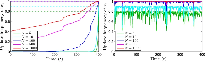
Figure 1: Update rates for xt versus t∈ {1, . . . ,400} for PG (left) and for PGAS (right).
The dashed lines correspond to the ideal rates (N −1)/N. (This figure is best viewed in color.)
empirical evaluation of PGAS is provided in Section 7. Consider the one-dimensional linear Gaussian state-space (LGSS) model,
xt+1 =axt+vt, vt∼ N(0, σv2),
yt=xt+et et∼ N(0, σe2),
where the state process {xt}t≥1 is latent and observations are made only via the
measure-ment process {yt}t≥1. For simplicity, the parameters θ = (a, σv, σe) = (0.9,0.32,1) are
assumed to be known. A batch of T = 400 observations are simulated from the system. Given these, we seek the joint smoothing density p(x1:T |y1:T). To generate samples from
this density we employ both PG and PGAS with varying number of particles ranging from N = 5 to N = 1 000. We simulate sample paths of length 1 000 for each algorithm. To compare the mixing, we look at the update rate of xt versus t, which is defined as the
proportion of iterations wherextchanges value. The results are reported in Figure 1, which
reveals that AS significantly increases the probability of updatingxt fortfar from T.
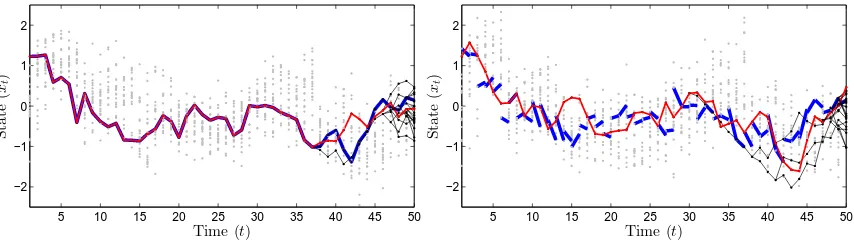
The poor update rates for PG is a manifestation of the well-known path degeneracy problem of SMC samplers (see, e.g., Doucet and Johansen 2011). Consider the process of sampling from the PG kernel for a fixed reference trajectory x01:T. A particle system generated by the PG algorithm (corresponding to Algorithm 2, but with line 8 replaced with aNt =N) is shown in Figure 2 (left). For clarity of illustration, we have used a small number of particles and time steps, N = 20 and T = 50, respectively. By construction, the reference trajectory (shown by a thick blue line) is retained throughout the sampling procedure. As a consequence, the particle system degenerates toward this trajectory which implies thatx?1:T (shown as a red line) to a large extent will be identical tox01:T.
5 10 15 20 25 30 35 40 45 50 −2
−1 0 1 2
Time (t)
S
tat
e
(
xt
)
5 10 15 20 25 30 35 40 45 50 −2
−1 0 1 2
Time (t)
S
tat
e
(
xt
)
Figure 2: Particle systems generated by the PG algorithm (left) and by the PGAS algorithm (right), for the same reference trajectoryx01:T (shown as a thick blue line in the left panel, partly underneath the red line). The gray dots show the particle positions and the thin black lines show the ancestral dependencies of the particles. The extracted trajectory x?1:T is illustrated with a red line. In the right panel, AS has the effect of breaking the reference trajectory into pieces, causing the particle system to degenerate toward something different thanx01:T. (This figure is best viewed in color.)
blue lines are again used to illustrate the reference particles, but now with updated ancestor indices. That is, the blue line segments are drawn between xaNt
t−1 and x0t fort ≥ 2. It can
be seen that the effect of AS is that, informally, the reference trajectory is broken into pieces. It is worth pointing out that the particle system still collapses; AS does not prevent path degeneracy. However, it causes the particle system to degenerate toward something different than the reference trajectory. As a consequence, x?
1:T (shown as a red line in the
figure) will with high probability be substantially different fromx01:T, enabling high update rates and thereby much faster mixing.
4. Theoretical Justification
In this section we investigate the invariance and ergodicity properties of the PGAS kernel.
4.1 Stationary Distribution
We begin by stating a theorem, whose proof is provided later in this section, which shows that the invariance property of PG is not violated by the AS step.
Theorem 1. For any N ≥1 andθ∈Θ, the PGAS kernel PθN leaves ¯γθ,T invariant:
¯
γθ,T(B) =
Z
An apparent difficulty in establishing this result is that it is not possible to write down a simple, closed-form expression forPθN. In fact, the PGAS kernel is given by
PθN(x01:T, B) =Eθ,x01:T
h
1B(xk1:T)
i
, (4)
where1Bis the indicator function for the setB ∈ XT and whereEθ,x01:T denotes expectation
with respect to all the random variables generated by Algorithm 2, i.e., all the particles
x1:T and ancestor indices a2:T, as well as the index k. Computing this expectation is not
possible in general. Instead of working directly with (4), however, we can adopt the strategy employed by Andrieu et al. (2010). That is, we treat all the random variables generated by Algorithm 2,{x1:T,a2:T, k}, as auxiliary variables, thus avoiding an intractable integration.
In the following, it is convenient to view xNt as a random variable with distributionδx0
t.
Recall that the particle trajectory xk1:T is the ancestral path of the particlexkT. That is, we can write
xk1:T =xb1:T
1:T ,(x b1
1 , . . . , x bT
T ),
where the indicesb1:T are given recursively by the ancestor indices: bT =kand bt=abt+1t+1.
Let Ω , XN T × {1, . . . , N}N(T−1)+1 be the space of all random variables generated by
Algorithm 2. Following Andrieu et al. (2010), we then define a probability density function φθ: Ω7→Ras follows:
φθ(x1:T,a2:T, k) =φθ(x1:b1:TT , b1:T)φθ(x−1:bT1:T,a −b2:T
2:T |x b1:T
1:T , b1:T)
, γ¯θ,T(x
b1:T
1:T )
NT
| {z }
marginal N
Y
i=1 i6=b1
rθ,1(xi1) T
Y
t=2 N
Y
i=1 i6=bt
Mθ,t(ait, xit)
| {z }
conditional
, (5)
where we have introduced the notation
x−ti ={x1t, . . . , xit−1, xit+1, . . . , xNt }, x−b1:T
1:T ={x −b1
1 , . . . , x −bT
T },
and similarly for the ancestor indices. By construction,φθ is nonnegative and integrates to
one, i.e., φθ is indeed a probability density function on Ω. We refer to this density as the
extended target density.
The factorization into a marginal and a conditional density is intended to reveal some of the structure inherent in the extended target density. In particular, the marginal density of the variables{xb1:T
1:T , b1:T}is defined to be equal to the original target density ¯γθ,T(x b1:T
1:T ),
up to a factor N−T corresponding to a uniform distribution over the index variables b1:T.
This has the important implication that if {x1:T,a2:T, k} are distributed according to φθ,
then, by construction, the marginal distribution ofxb1:T
1:T is ¯γθ,T.
By constructing an MCMC kernel with invariant distribution φθ, we will thus obtain
a kernel with invariant distribution ¯γθ,T (the PGAS kernel) as a byproduct. To prove
of Lemma 2 below, but basically it refers to the process of marginalizing out some of the variables of the model in the individual steps of the Gibbs sampler. This is done in such a way that it does not violate the invariance property of the Gibbs kernel, i.e., each such Gibbs step will leave the extended target distribution invariant. As a consequence, the invariance property of the PGAS kernel follows. First we show that the PGAS algorithm in fact implements the following sequence of partially collapsed Gibbs steps for φθ.
Procedure 1 (Instrumental reformulation of PGAS). Given x0,b 0
1:T
1:T ∈ XT and b 0 1:T ∈
{1, . . . , N}T:
(i) Drawx−b
0
1
1 ∼φθ(· |x 0,b0
1:T
1:T , b01:T) and, for t= 2 to T, draw:
{x−bt
t ,a −bt
t } ∼φθ(· |x −b01:t−1
1:t−1 ,a2:t−1, x 0,b0
1:T
1:T , b 0 t−1:T),
abt
t ∼φθ(· |x −b0
1:t−1
1:t−1 ,a2:t−1, x 0,b0
1:T
1:T , b 0 t:T),
(ii) Drawk∼φθ(· |x1:−bT1:T,a2:T, x 0,b01:T 1:T ).
Lemma 1. Algorithm 2 is equivalent to the partially collapsed Gibbs sampler of Procedure 1, conditionally onx0,b
0
1:T
1:T =x01:T and b01:T = (N, . . . , N). Proof. From (5) we have, by construction,
φθ(x−1:bT1:T,a−2:Tb2:T |xb1:1:TT , b1:T) = N
Y
i=1 i6=b1
rθ,1(xi1) T Y t=2 N Y i=1 i6=bt
Mθ,t(ait, xit).
By marginalizing this expression over{x−bt+1:T
t+1:T ,a −bt+1:T
t+1:T } we get
φθ(x−1:bt1:t,a −b2:t
2:t |x b1:T
1:T , b1:T) = N
Y
i=1 i6=b1
rθ,1(xi1) t Y s=2 N Y i=1 i6=bs
Mθ,s(ais, xis),
It follows that
φθ(x−1b1 |x b1:T
1:T , b1:T) = N
Y
i=1 i6=b1
rθ,1(xi1), (6a)
and, fort= 2, . . . , T,
φθ(x−tbt,a −bt
t |x −b1:t−1
1:t−1 ,a −b2:t−1
2:t−1 , x b1:T
1:T , b1:T)
= φθ(x
−b1:t
1:t ,a −b2:t
2:t |x b1:T
1:T , b1:T)
φθ(x −b1:t−1
1:t−1 ,a −b2:t−1
2:t−1 |x b1:T
1:T , b1:T)
=
N
Y
i=1 i6=bt
Mθ,t(ait, xit). (6b)
Hence, we can sample from (6a) and (6b) by drawing xi1 ∼rθ,1(·) for i ∈ {1, . . . , N} \b1
bt =N for t= 1, . . . , T, the initialization at line 1 and the particle propagation at line 5
of Algorithm 2 correspond to sampling from (6a) and (6b), respectively. Next, we consider the AS step. Recall that abt
t identifies to bt−1. We can thus write
φθ(abtt |x1:t−1,a2:t−1, xbt:t:TT , bt:T)∝φθ(x1:t−1,a2:t−1, xbt:t:TT , bt−1:T)
=φθ(xb1:1:TT , b1:T)φθ(x −b1:t−1
1:t−1 ,a −b2:t−1
2:t−1 |x b1:T
1:T , b1:T)
= γθ,T(x
b1:T
1:T )
γθ,t−1(xb1:1:tt−1−1)
γθ,t−1(xb1:1:tt−1−1)
Zθ,TNT N
Y
i=1 i6=b1
rθ,1(xi1) t−1 Y s=2 N Y i=1 i6=bs
Mθ,s(ais, xis). (7)
To simplify this expression, note first that we can write
γθ,t−1(x1:t−1) =γθ,1(x1) t−1
Y
s=2
γθ,s(x1:s)
γθ,s−1(x1:s−1)
.
By using the definition of the weight function (2), this expression can be expanded according to
γθ,t−1(x1:t−1) =Wθ,1(x1)rθ,1(x1) t−1
Y
s=2
Wθ,s(x1:s)rθ,s(xs|x1:s−1).
Plugging the trajectoryxb1:t−1
1:t−1 into the above expression, we get
γθ,t−1(xb1:1:tt−1−1) =w1b1rθ,1(xb11) t−1
Y
s=2
wbs
s rθ,s(xbss |x b1:s−1
1:s−1)
= t−1 Y s=1 N X l=1
wls !
wb1
1
P
lw1l
rθ,1(xb11) t−1
Y
s=2
wbs
s
P
lwls
rθ,s(xbss |x b1:s−1
1:s−1)
= w
bt−1
t−1
P
lwlt−1 t−1 Y s=1 N X l=1
wls !
rθ,1(xb11) t−1
Y
s=2
Mθ,s(abss, xbss). (8)
Expanding the numerator in (7) according to (8) results in
φθ(abtt |x1:t−1,a2:t−1, xbt:t:TT , bt:T)
∝ γθ,T(x
b1:T
1:T )
γθ,t−1(xb1:1:tt−1−1)
wbt−1
t−1
P
lwlt−1
Qt−1
s=1
P
lwsl
Zθ,TNT N
Y
i=1
rθ,1(xi1) t−1 Y s=2 N Y i=1
Mθ,s(ais, xis)
∝wbt−1
t−1
γθ,T((xb1:1:tt−1−1, x bt:T
t:T ))
γθ,t−1(xb1:1:tt−1−1)
. (9)
Consequently, with bt=N and xtb:t:TT =x0t:T, sampling from (9) corresponds to the AS step
of line 8 of Algorithm 2. Finally, analogously to (9), it follows thatφθ(k|x1:T,a2:T)∝wkT,
Next, we show that Procedure 1 leavesφθinvariant. This is done by concluding that the
procedure is a properly collapsed Gibbs sampler; see Dyk and Park (2008). Marginalization, or collapsing, is commonly used within Gibbs sampling to improve the mixing and/or to simplify the sampling procedure. However, it is crucial that the collapsing is carried out in the correct order to respect the dependencies between the variables of the model.
Lemma 2. The Gibbs sampler of Procedure 1 is properly collapsed and thus leaves φθ
invariant.
Proof. Consider the following sequence ofcomplete Gibbs steps:
(i) Draw {x−b
0
1
1 ,x −b0
2:T
2:T ,a −b0
2:T
2:T } ∼φθ(· |x 0,b0
1:T
1:T , b 0
1:T) and, fort= 2 to T, draw:
{x−bt
t ,at,x −b0t+1:T t+1:T ,a
−b0t+1:T
t+1:T } ∼φθ(· |x −b01:t−1
1:t−1 ,a2:t−1, x 0,b01:T 1:T , b
0 t:T).
(ii) Draw k∼φθ(· |x −b0
1:T
1:T ,a2:T, x 0,b0
1:T
1:T ).
In the above, all the samples are drawn from conditionals under the full joint density φθ(x1:T,a2:T, k). Hence, it is clear that the above procedure will leave φθ invariant. Note
that some of the variables above have been marked by an underline. It can be seen that these variables are in fact never conditioned upon in any subsequent step of the procedure. That is, the underlined variables are never used. Therefore, to obtain a valid sampler it is sufficient to sample all the non-underlined variables from their respective marginals. Furthermore, from (6b) it can be seen that{x−bt
t ,a −bt
t }are conditionally independent ofa bt
t ,
i.e., it follows that the complete Gibbs sweep above is equivalent to the partially collapsed Gibbs sweep of Procedure 1. Hence, the Gibbs sampler is properly collapsed and it will
therefore leaveφθ invariant.
Proof (Theorem 1). Let L(dx−b
0
1:T
1:T , da2:T, dk | x01:T, b 0
1:T) denote the law of the random
variables generated by Procedure 1, conditionally on x0,b 0
1:T
1:T = x 0
1:T and on b01:T. Using
Lemma 2 and recalling that φθ(xb1:1:TT , b1:T) =N−T¯γθ,T(xb1:1:TT ) we have
¯
γθ,T(B) =
Z
1B(xk1:T)L(dx −b0
1:T
1:T , da2:T, dk |x 0 1:T, b
0 1:T)
×δx0
1(dx
b01
1 )· · ·δx0
T(dx
b0
T
T )
¯
γθ,T(x01:T)
NT dx 0 1:Tdb
0
1:T, ∀B ∈ XT. (10)
By Lemma 1 we know that Algorithm 2, which implicitly defines PN
θ , is equivalent to
Procedure 1 conditionally onx0,b 0
1:T
1:T =x 0
1:T and b 0
1:T = (N, . . . , N). That is to say,
PθN(x01:T, B) = Z
1B(xk1:T)L(dx
−(N, ..., N)
1:T , da2:T, dk|x 0
1:T,(N, . . . , N))
×δx01(dxN1 )· · ·δx0T(dxNT),
some other positions, when enumerating the particles.2 This implies that for any b01:T ∈ {1, . . . , N}T,
PθN(x01:T, B) = Z
1B(xk1:T)L(dx −b0
1:T
1:T , da2:T, dk |x1:0 T, b01:T)δx0
1(dx
b01
1 )· · ·δx0
T(dx
b0
T
T ). (11)
Plugging (11) into (10) gives the desired result,
¯
γθ,T(B) =
Z
PθN(x01:T, B)¯γθ,T(x01:T)
X
b0
1:T
1 NT
| {z }
=1
dx01:T, ∀B∈ XT.
4.2 Ergodicity
To show ergodicity of the PGAS kernel we need to characterize the support of the target and the proposal densities. Let,
Sθ,t={x1:t∈Xt: ¯γθ,t(x1:t)>0},
Qθ,t={x1:t∈Xt:rθ,t(xt|x1:t−1)¯γθ,t−1(x1:t−1)>0},
with obvious modifications fort= 1. The following is a minimal assumption.
(A1) For any θ∈Θ andt∈ {1, . . . , T}we have Sθ t ⊆ Qθt.
Assumption (A1) basically states that the support of the proposal density should cover the support of the target density. Ergodicity of PG under Assumption (A1) has been established by Andrieu et al. (2010). The same argument can be applied also to PGAS.
Theorem 2 (Andrieu et al. (2010, Theorem 5)). Assume (A1). Then, for anyN ≥2 and
θ∈Θ, PθN is γ¯θ,T-irreducible and aperiodic. Consequently,
lim
n→∞k(P N θ )n(x
0
1:T,·)−γ¯θ,T(·)kTV= 0, ¯γθ,T-a.a. x01:T.
To strengthen the ergodicity results for the PGAS kernel, we use a boundedness con-dition for the importance weights, given in assumption (A2) below. Such a concon-dition is typical also in classical importance sampling and is, basically, a stronger version of assump-tion (A1).
(A2) For any θ ∈ Θ and t ∈ {1, . . . , T}, there exists a constant κθ < ∞ such that
kWθ,tk∞≤κθ.
Theorem 3. Assume (A2). Then, for any N ≥ 2 and θ ∈ Θ, PθN is uniformly ergodic. That is, there exist constants Rθ<∞ andρθ∈[0,1)such that
k(PθN)n(x1:0 T,·)−γ¯θ,T(·)kTV≤Rθρnθ, ∀x01:T ∈XT.
Proof. We show that PθN satisfies a Doeblin condition,
PθN(x01:T, B)≥εθ¯γθ,T(B), ∀x01:T ∈XT,∀B ∈ XT, (12)
for some constant εθ > 0. Uniform ergodicity then follows from Tierney (1994,
Proposi-tion 2). To prove (12) we use the representaProposi-tion of the PGAS kernel in (4),
PθN(x01:T, B) =Eθ,x0
1:T
h
1B(xk1:T)
i =
N
X
j=1 Eθ,x0
1:T
" wTj P
lwlT
1B(xj1:T)
#
≥ 1
N κθ N−1
X
j=1 Eθ,x0
1:T
h
wjT1B(xj1:T)
i
= N−1 N κθ Eθ,x
0
1:T
Wθ,T(x11:T)1B(x11:T)
. (13)
Here, the inequality follows from bounding the weights in the normalization byκθ and by
simply discarding theNth term of the sum (which is clearly nonnegative). The last equality follows from the fact that the particle trajectories {xi1:T}Ni=1−1 are equally distributed under Algorithm 2. Lethθ,t :Xt7→R+ and consider
Eθ,x0
1:T
hθ,t(x11:t)
=Eθ,x0
1:T
h
Eθ,x0
1:T
hθ,t(x11:t)|x1:t−1,a2:t−1
i
=Eθ,x0
1:T N X j=1 Z
hθ,t((xj1:t−1, xt))
wjt−1 P
lwtl−1
rθ,t(xt|xj1:t−1)dxt
≥ N−1
N κθ Eθ,x
0
1:T
Z
hθ,t((x11:t−1, xt))Wθ,t−1(x1:1t−1)rθ,t(xt|x11:t−1)dxt
, (14)
where the inequality follows analogously to (13). Now, let
hθ,T(x1:T) =Wθ,T(x1:T)1B(x1:T),
hθ,t−1(x1:t−1) =
Z
hθ,t(x1:t)Wθ,t−1(x1:t−1)rθ,t(xt|x1:t−1)dxt, t≤T.
Then, by iteratively making use of (14) and changing the order of integration, we can bound (13) according to
N−1
N κθ
−T
PθN(x01:T, B)≥Eθ,x01:T
hθ,1(x11)
= Z
Wθ,1(x1)rθ,1(x1) T
Y
t=2
(Wθ,t(x1:t)rθ,t(xt|x1:t−1))1B(x1:T)dx1:T
= Z
γθ,1(x1) T
Y
t=2
γθ,t(x1:t)
γθ,t−1(x1:t−1)
1B(x1:T)dx1:T
= Z
γθ,T(x1:T)1B(x1:T)dx1:T =Zθ,T¯γθ,T(B).
5. PGAS for State-Space Models
SSMs comprise an important special case of the model class treated above. In this section, we illustrate how PGAS can be used for inference and learning of these models.
5.1 Sampling from the Joint Smoothing Distribution with PGAS
Consider the (possibly) nonlinear/non-Gaussian SSM
xt+1∼fθ(xt+1|xt), (15a)
yt∼gθ(yt|xt), (15b)
and x1 ∼ µθ(x1), where θ ∈ Θ is a static parameter, xt is the latent state and yt is the
observation at timet, respectively. Given a batch of measurements y1:T, we wish to make
inferences about θ and/or about the latent states x1:T. In the subsequent section we will
provide both a Bayesian and a frequentist learning algorithm based on the PGAS kernel. However, we start by discussing how to implement the PGAS algorithm for this specific model.
For an SSM the target distribution of interest is typically the joint smoothing distri-bution pθ(x1:T |y1:T). Consequently, since pθ(x1:T |y1:T) ∝pθ(x1:T, y1:T), the sequence of
unnormalized target densities is given by
γθ,t(x1:t) =pθ(x1:t, y1:t), t= 1, . . . , T. (16)
As we have previously discussed, the process of sampling from the PGAS kernel is similar to running a PF. The only non-standard (and nontrivial) operation is the AS step. By plugging the specific choice of unnormalized target densities (16) into the general expression for the AS weights (3), we get
e
wit−1|T =wit−1
pθ((xi1:t−1, x0t:T), y1:T)
p(xi
1:t−1, y1:t−1)
=wti−1pθ(xt0:T, yt:T |xit−1)∝wit−1fθ(x0t|xit−1). (17)
This expression can be understood as an application of Bayes’ theorem. Recall that we want to assign an ancestor at timet−1 to the reference particlex0t. The importance weight wit−1 is the prior probability of the particlexit−1 and the factorfθ(x0t|xit−1) is the likelihood
of moving from xit−1 to x0t. The product of these two factors is thus proportional to the posterior probability that x0t originated fromxit−1, which gives us the AS probability.
For concreteness we provide a restatement of the PGAS algorithm, specifically for the case of SSMs, in Algorithm 3. To highlight the similarities between PGAS and a standard PF, we have chosen to present Algorithm 3 using a notation and nomenclature that is com-mon in the particle filtering literature, but that differs slightly from our previous notation. However, we emphasize that Algorithm 3 is completely equivalent to Algorithm 2 when the target distributions are given by (16). Note that the computational cost of the AS step is O(N) per time step, i.e., of the same order as the PF. Consequently, for an SSM, the computational complexity of PGAS is the same as for PG, in total O(N T).
Algorithm 3 PGAS Markov kernel for the joint smoothing distribution pθ(x1:T |y1:T) Input: Reference trajectory x01:T ∈XT and parameter θ∈Θ.
Output: Samplex?1:T ∼PθN(x01:T,·) from the PGAS Markov kernel. 1: Draw xi1 ∼rθ,1(x1 |y1) for i= 1, . . . , N −1.
2: SetxN1 =x01.
3: Setwi1=gθ(y1|xi1)µθ(xi1)/rθ,1(x1i |y1) fori= 1, . . . , N.
4: fort= 2 toT do
/* Resampling and ancestor sampling */ 5: Generate {exi
1:t−1}Ni=1−1 by sampling N −1 times with replacement from {xi1:t−1}Ni=1
with probabilities proportional to the importance weights {wit−1}N i=1.
6: Draw J with
P(J =i) =
wit−1fθ(x0t|xit−1)
P
l=1wtl−1fθ(x0t|xlt−1)
, i=1, . . . , N
and set exN1:t−1 =xJ1:t−1. /* Particle propagation */ 7: Simulate xit∼rθ,t(xt|ex
i
t−1, yt) for i= 1, . . . , N−1.
8: SetxNt =x0t. 9: Setxi1:t= (xe
i
1:t−1, xit) for i= 1, . . . , N.
/* Weighting */ 10: Setwi
t=gθ(yt|xti)fθ(xit|xe
i
t−1)/rθ,t(xit|xe
i
t−1, yt) fori= 1, . . . , N.
11: end for
12: Draw kwithP(k=i)∝wTi.
13: return x?
1:T =xk1:T.
5.2 Learning Algorithms for State-Space Models
We now turn to the problem of learning the model parameter θ in the SSM (15), given a batch of observations y1:T. Consider first the Bayesian setting where a prior distribution
π(θ) is assigned toθ. We seek the parameter posteriorp(θ|y1:T) or, more generally, the joint
state and parameter posteriorp(θ, x1:T |y1:T). Gibbs sampling can be used to simulate from
this distribution by sampling the state variables {xt} one at a time and the parameters θ
Algorithm 4 PGAS for Bayesian learning of SSMs 1: Setθ[0] and x1:T[0] arbitrarily.
2: forn≥1do
3: Draw x1:T[n]∼PθN[n−1](x1:T[n−1],·). /* By running Algorithm 3 */
4: Draw θ[n]∼p(θ|x1:T[n], y1:T).
5: end for
poor mixing, due to the often high autocorrelation of the state sequence. The PGAS kernel offers a different approach, namely to sample the complete state trajectory x1:T in one
block. This can considerably improve the mixing of the sampler (de Jong and Shephard, 1995). Due to the invariance and ergodicity properties of the kernel (Theorems 1– 3), the validity of the Gibbs sampler is not violated. We summarize the procedure in Algorithm 4. PGAS is also useful for maximum-likelihood-based learning of SSMs. A popular strategy for computing the maximum likelihood estimator
b
θML= arg max θ∈Θ
logpθ(y1:T)
is to use the expectation maximization (EM) algorithm (Dempster et al., 1977; McLachlan and Krishnan, 2008). EM is an iterative method, which maximizes logpθ(y1:T) by iteratively
maximizing an auxiliary quantity: θ[n] = arg maxθ∈ΘQ(θ, θ[n−1]), where
Q(θ, θ[n−1]) = Z
logpθ(x1:T, y1:T)pθ[n−1](x1:T |y1:T)dx1:T.
When the above integral is intractable to compute, one can use a Monte Carlo approximation or a stochastic approximation of the intermediate quantity, leading to the MCEM (Wei and Tanner, 1990) and the SAEM (Delyon et al., 1999) algorithms, respectively. When the underlying Monte Carlo simulation is computationally involved, SAEM is particularly useful since it makes efficient use of the simulated values. The SAEM approximation of the auxiliary quantity is given by
b
Qn(θ) = (1−αn)Qbn−1(θ) +αnlogpθ(x1:T[n], y1:T), (18)
whereαnis the step size and, in the vanilla form of SAEM, x1:T[n] is drawn from the joint
smoothing density pθ[n−1](x1:T | y1:T). In practice, the stochastic approximation update
(18) is typically made on some sufficient statistic for the complete data log-likelihood; see Delyon et al. (1999) for details. While the joint smoothing density is intractable for a general nonlinear/non-Gaussian SSM, it has been recognized that it is sufficient to sample from a uniformly ergodic Markov kernel, leaving the joint smoothing distribution invariant (Benveniste et al., 1990; Andrieu et al., 2005). A practical approach is therefore to compute the auxiliary quantity according to the stochastic approximation (18), but where x1:T[n]
is simulated from the PGAS kernel PθN[n−1](x1:T[n−1],·). This particle SAEM algorithm,
previously presented by Lindsten (2013), is summarized in Algorithm 5.
6. Beyond State-Space Models
Algorithm 5 PGAS for frequentist learning of SSMs 1: Setθ[0] and x1:T[0] arbitrarily. Set Qb0(θ)≡0. 2: forn≥1do
3: Draw x1:T[n]∼PθN[n−1](x1:T[n−1],·). /* By running Algorithm 3 */
4: Compute Qbn(θ) according to (18). 5: Compute θ[n] = arg maxθ∈ΘQbn(θ). 6: if convergence criterion is met then
7: return θ[n]. 8: end if
9: end for
dependencies between the latent variables, however, this is not the case and the general expression (3) needs to be used. In this section we consider the computational aspects of the AS step, first in a very general setting and then specifically for the class of non-Markovian latent variable models.
6.1 Modifications and Mixed Strategies
The interpretation of the PGAS algorithm as a standard MCMC sampler on an extended space opens up for straightforward modifications of the algorithm while still making sure that it retains its desirable theoretical properties. In particular, for models where the computation of the AS weights in (3) is costly—that is, when evaluating the unnormalized joint target densityγθ,T is computationally involved—it can be beneficial to modify the AS
step to reduce the overall computational cost of the algorithm. Let
ρ(i) = we
i t−1|T
PN
l=1we
l t−1|T
, i= 1, . . . , N, (19)
denote the law of the ancestor indexaNt , sampled at line 8 of Algorithm 2. From Lemma 1, we know that this step of the algorithm in fact corresponds to a Gibbs step for the extended target distribution (5). To retain the correct limiting distribution of the PGAS kernel, it is therefore sufficient thataN
t is sampled from a Markov kernel leaving (19) invariant (resulting
in a standard combination of MCMC kernels; see, e.g., Tierney 1994).
A simple modification is to carry out the AS step only for a fraction of the time steps. For instance, we can generate the ancestor indexaN
t according to:
(
With probability 1−η, set aNt =N,
Otherwise, simulateaNt with P(aNt =i) =ρ(i),
(20)
rates for the complete trajectory (cf. Figure 1 where we get high update rates for PG for the last few time steps, even when using a small number of particles). We illustrate this empirically in the simulation study in Section 7.3.
Another modification, that can be used either on its own or in conjunction with (20), is to use MH to simulate from (19). Letq(i0|i) be an MH proposal kernel on{1, . . . , N}. We can thus propose a move for the ancestor indexaNt , fromN toi0, by simulatingi0 ∼q(· |N). With probability
1∧we
i0
t−1|T
e wN
t−1|T
q(N |i0)
q(i0 |N) (21)
the sample is accepted and we setaNt =i0, otherwise we keep the ancestry aNt =N. Using this approach, we avoid computing the normalizing constant in (19), i.e., we only need to evaluate the AS weights for the proposed values. This will reduce the computational cost of the AS step by, roughly, a factorN which can be very useful wheneverN is moderately large. Since the variable aNt is discrete-valued, it is recommended to use a forced move proposal in the spirit of Liu (1996). That is, q is constructed so that q(i|i) = 0,∀i, ensuring that the current state of the chain is not proposed anew, which would be a wasteful operation.
6.2 Non-Markovian Latent Variable Models
A very useful generalization of SSMs is the class of non-Markovian latent variable models,
xt+1∼fθ(xt+1 |x1:t),
yt∼gθ(yt|x1:t).
Similarly to the SSM (15), this model is characterized by a latent process xt ∈ X and an
observed processyt∈Y. However, it does not share the conditional independence properties
that are central to SSMs. Instead, both the transition density fθ and the measurement
density gθ may depend on the entire past history of the latent process. Below we discuss
the AS step of the PGAS algorithm specifically for these non-Markovian models and derive a truncation strategy for the AS weights. First, however, to motivate the present development we review some application areas in which this type of models arise.
In Bayesian nonparametrics (Hjort et al., 2010) the latent random variables of the classical Bayesian model are replaced by latent stochastic processes, which are typically non-Markovian. This includes popular models based on the Dirichlet process, e.g., Teh et al. (2006); Escobar and West (1995), and Gaussian process regression and classification models (Rasmussen and Williams, 2006). These processes are also commonly used as components in hierarchical Bayesian models, which then inherit their non-Markovianity. An example is the Gaussian process SSM (Turner and Deisenroth, 2010; Frigola et al., 2013), a flexible nonlinear dynamical systems model, for which PGAS has been successfully applied (Frigola et al., 2013).
an SSM in terms of its “innovations” (i.e., the driving noise of the state process), it is possible to use backward and ancestor sampling in models for which the state transition density is not available. This includes many models for which the transition is implicitly given by a simulator (Gander and Stephens, 2007; Fearnhead et al., 2008; Golightly and Wilkinson, 2008; Murray et al., 2013) or degenerate models where the transition density does not even exist (Ristic et al., 2004; Gustafsson et al., 2002). We illustrate these ideas in Section 7. See also Lindsten and Sch¨on (2013, Section 4) for a more in-depth discussion on reformulations of SSMs as non-Markovian models.
Finally, it is worth to point out that many statistical models which are not sequential “by nature” can be conveniently viewed as non-Markovian latent variable models. This includes, among others, probabilistic graphical models such as Markov random fields; see Lindsten and Sch¨on (2013, Section 4).
To employ PGAS, or in fact any backward-simulation-based method (see Lindsten and Sch¨on 2013), we need to evaluate the AS weights (3) which depend on the ratio
γθ,T(x1:T)
γθ,t−1(x1:t−1)
= pθ(x1:T, y1:T) pθ(x1:t−1, y1:t−1)
=
T
Y
s=t
gθ(ys|x1:s)fθ(xs|x1:s−1). (22)
Assuming that gθ and fθ can both be evaluated in constant time, the computational cost
of computing the backward sampling weights (3) will thus be O(N T). This implies that the overall computational complexity of the PGAS kernel will scale quadratically with T which can be prohibitive in some cases. The general strategies discussed in Section 6.1, i.e., using AS sporadically and/or using MH within PGAS, can of course be used to mitigate this issue. Nonetheless, the AS step can easily become the computational bottleneck when applying the PGAS algorithm to a non-Markovian model.
To make further progress we consider non-Markovian models in which there is a decay in the influence of the past on the present, akin to that in Markovian models but without the strong Markovian assumption. Hence, it is possible to obtain a useful approximation of the AS weights by truncating the product (22) to a smaller number of factors, say `. We can thus replace (3) with the approximation
e
wt`,i−1|T ,wti−1
γθ,t−1+`((xi1:t−1, x0t:t−1+`))
γθ,t−1(xi1:t−1)
=wti−1 t−1+`
Y
s=t
gθ(ys|xi1:t−1, x0t:s)fθ(x0s|xi1:t−1, x0t:s−1). (23)
Let ρb`(k) be the probability distribution defined by the truncated AS weights (23),
analo-gously to (19). The following proposition formalizes our assumption.
Proposition 1. Let hs(k) = gθ(yt−1+s | xk1:t−1, x0t:t−1+s)fθ(x0t−1+s | xk1:t−1, x0t:t−1+s) and
assume thatmaxk,l(hs(k)/hs(l)−1)≤Aexp(−cs), for some constantsA andc >0. Then,
DKLD(ρkρb`) ≤Cexp(−c`) for some constant C, where DKLD is the Kullback-Leibler (KL)
divergence.
0 50 100 150 200 0
0.2 0.4 0.6 0.8 1
ℓadpt.= 5
P
ro
b
a
b
il
it
y
Truncation level (ℓ)
0 50 100 150 200
ℓadpt.= 12
Truncation level (ℓ)
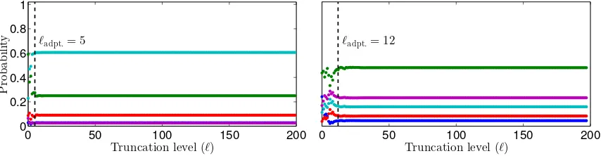
Figure 3: Probability under ρb` as a function of the truncation level ` for two different
systems; one 5-dimensional (left) and one 20-dimensional (right). The N = 5 dotted lines correspond to ρb`(k) for k ∈ {1, . . . , N}, respectively (N.B. two of
the lines overlap in the left figure). The dashed vertical lines show the value of the truncation level`adpt., resulting from the adaption scheme with υ= 0.1 and
τ = 10−2. See Section 7.2 for details on the experiments.
Using the approximation given by (23), the AS weights can be computed in constant time within the PGAS framework. The resulting approximation can be quite useful; indeed, in our experiments we have seen that even`= 1 can lead to very accurate inferential results. In general, however, it will not be known a priori how to set the truncation level `. To address this problem, we propose to use an adaptive strategy. Since the approximative weights (23) can be evaluated sequentially, the idea is to start with`= 1 and then increase `until the weights have, in some sense, converged. In particular, in our experimental work, we have used the following simple approach.
Let ε` =DTV(ρb`,ρb`−1) be the total variation (TV) distance between the approximative AS distributions for two consecutive truncation levels. We then compute the exponentially decaying moving average of the sequenceε`, with forgetting factorυ∈[0,1], and stop when
this falls below some threshold τ ∈ [0,1]. This adaption scheme removes the requirement to specify `directly, but instead introduces the design parameters υand τ. However, these parameters are much easier to reason about—a small value forυ gives a rapid response to changes in ε` whereas a large value gives a more conservative stopping rule, improving the
accuracy of the approximation at the cost of higher computational complexity. A similar tradeoff holds for the thresholdτ as well. Most importantly, we have found that the same values for υ and τ can be used for a wide range of models, with very different mixing properties.
To illustrate the effect of the adaption rule, and how the distributionρb`typically evolves
The approximation (23) can be used in a few different ways. First, as discussed above, we can simply replaceρwithρb` in the PGAS algorithm, resulting in a total computational cost ofO(N T `). This is the approach that we have favored, owing to its simplicity and the fact that we have found the truncation to lead to very accurate approximations. Another approach, however, is to use ρb` as an efficient proposal distribution for the MH algorithm suggested in Section 6.1, leading to an O(N T `+T2) complexity. The MH accept/reject decision will then compensate for the approximation error caused by the truncation. A third approach is to use the MH algorithm, but to make use of the approximation (23) when evaluating the acceptance probability (21). By doing so, the algorithm can be implemented withO(N T +T `) computational complexity.
7. Numerical Evaluation
In this section we illustrate the properties of PGAS in a simulation study. First, in Sec-tion 7.1 we consider a stochastic volatility SSM and investigate the improvement in mixing offered by AS when PGAS is compared with PG. We do not consider PGBS in this example since, as we show in Proposition 2 in Appendix A, PGAS and PGBS are probabilistically equivalent in this scenario. The conditions of Proposition 2 imply that the weight function in the PF is independent of the ancestor indices. When applied to non-Markovian models, however, Proposition 2 does not apply, since the weight function then will depend on the complete history of the particles. PGAS and PGBS will then have different properties as is illustrated empirically in Section 7.2 where we consider inference in degenerate SSMs reformulated as non-Markovian models. Finally, in Section 7.3 we use a similar reformu-lation and apply PGAS for identification of an epidemiological model for which the state transition kernel is not available.
7.1 Stochastic Volatility Model with Leverage
Stochastic volatility (SV) models are commonly used to model the variation (or volatility) of a financial asset; see, e.g., Kim et al. (1998); Shephard (2005). Let rt be the price of
an asset at time t and let yt = log(rt/rt−1) denote the so-called log-returns. A typical SV
model is then given by the SSM:
xt+1 =µ(1−ϕ) +ϕxt+σvt,
yt= exp(−12xt)et,
vt
et
∼ N
0 0
,
1 ρ ρ 1
. (24)
The correlation between the process noise and the observation noise allows for a leverage effect by letting the price of the asset influence the future volatility. Assuming stationarity, the distribution of the initial state is given byµθ(x1) =N(x1;µ, σ2/(1−ϕ2)). The unknown
parameters of the model areθ= (µ, ϕ, σ2, ρ).
0 50 100 150 200 250 300 350 400 0
0.2 0.4 0.6 0.8 1
Lag
A
C
F
PG,T= 102
N= 5
N= 10
N= 100
N= 500
N= 1000
0 50 100 150 200 250 300 350 400
0 0.2 0.4 0.6 0.8 1
Lag
A
C
F
PGAS,T= 102
N= 5
N= 10
N= 100
N= 500
N= 1000
0 50 100 150 200 250 300 350 400
0 0.2 0.4 0.6 0.8 1
Lag
A
C
F
PG,T= 2011
N= 5
N= 10
N= 100
N= 500
N= 1000
0 50 100 150 200 250 300 350 400
0 0.2 0.4 0.6 0.8 1
Lag
A
C
F
PGAS,T= 2011
N= 5
N= 10
N= 100
N= 500
N= 1000
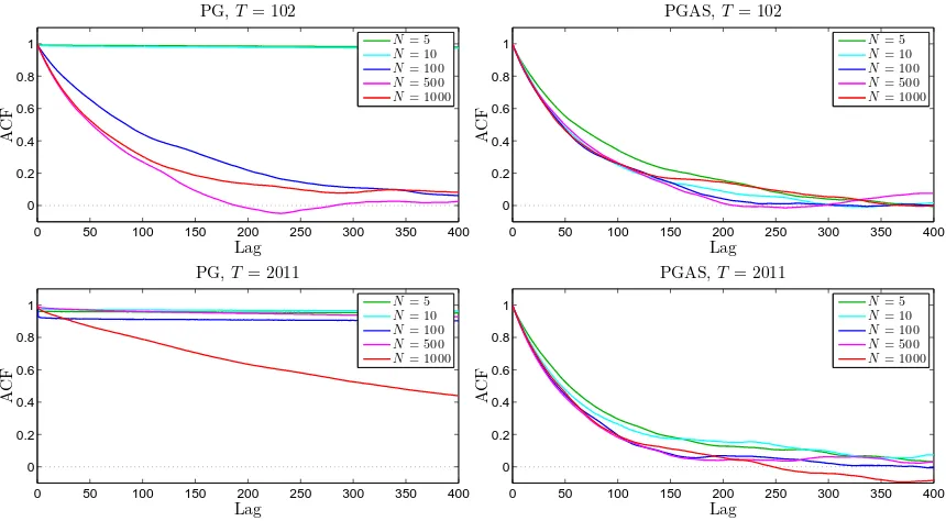
Figure 4: ACFs the parameter σ2 for PG (left column) and for PGAS (right column) for the S&P 500 data consisting of T = 102 (top row) and T = 2 011 (bottom row) observations, respectively. The results are reported for different number of particlesN. (This figure is best viewed in color.)
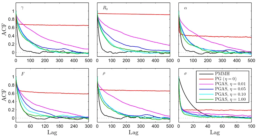
of T = 2 011 observations.3 We consider the the PGAS sampler (Algorithm 4) as well as the PG and PMMH samplers by Andrieu et al. (2010), all for a range of different number of particles, N ∈ {5,10,100,500,1 000}. All methods are simulated for 50 000 iterations, whereafter the first 10 000 samples are discarded as burn-in. For updatingθ, PG and PGAS simulate the parameters one at a time from their respective conditionals, whereas PMMH uses a Gaussian random walk tuned according to an initial trial run. Additional details on the experiments are given in Appendix C.
To evaluate the mixing of the samplers, we compute the autocorrelation functions (ACFs) for the sequences θ[n]−E[θ|y1:T].4 We start by considering the simpler problem
of analyzing a small subset of the data, consisting ofT = 102 samples (1/November/2013– 31/March/2014). The results for PG and PGAS for the parameter σ2 are reported in the
top row of Figure 4. Similar results hold for the other parameters as well. We see that the PG sampler requires a fairly large N to obtain good mixing and using N ≤10 causes the sampler to get completely stuck. For PGAS, on the other hand, the ACF is much more robust to the choice of N. Indeed, we obtain comparable mixing rates for any number of particles N ≥ 5. This suggests that the sampler in fact performs very closely to a fictive
3. The data was acquired from the Yahoo Finance web page https://finance.yahoo.com/q/hp?s= %5EGSPC&a=03&b=3&c=2006&d=02&e=31&f=2014&g=d
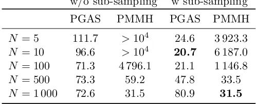
w/o sub-sampling w sub-sampling
PGAS PMMH PGAS PMMH
N = 5 111.7 >104 24.6 3 923.3
N = 10 96.6 >104 20.7 6 187.0
N = 100 71.3 4 796.1 21.1 1 146.8
N = 500 73.3 59.2 47.8 33.5
N = 1 000 72.6 31.5 80.9 31.5
Table 1: Average inefficiencies for the SV model.
“ideal” Gibbs sampler, i.e., a sampler that simulates x1:T from the true joint smoothing
distribution.
Next, we rerun the methods on the whole data set with T = 2 011 observations. The results are shown in the bottom row of Figure 4. The effect can be seen even more clearly in this more challenging scenario. Again, we find PGAS to perform very closely to an ideal Gibbs sampler for any N ≥5. In other words, for this model it is the mixing of the ideal Gibbs sampler, not the intrinsic particle approximation, that is the limitation of PGAS. The big difference in mixing between PG and PGAS can be understood as a manifestation of how they are affected by path degeneracy. These results are in agreement with the discussion in Section 3.3.
We now turn to a comparison between PGAS and PMMH. However, in doing so it is important to realize that these two methods, while both being instances of PMCMC, have quite different properties. In particular, just as PGAS can be thought of as an ap-proximation of an ideal Gibbs sampler, PMMH can be viewed as an apap-proximation of an ideal marginal MH sampler. Consequently, their respective performances depend on the properties of these ideal samplers and the preference for one method over the other heavily depends on the specific problem under study. Nevertheless, we apply both methods to the S&P 500 data (withT = 2 011). To evaluate the mixing, we compute5 theinefficiencies:
IF,1 + 2
∞
X
j=1
ACF(j)
for the four parameters of the model, whereACF(j) is the ACF at lagj. The interpretation of the inefficiency is that we needn×IF draws from the Markov chain to obtain the same precision as using ni.i.d. draws from the posterior. The average inefficiencies for the four parameters for PGAS and PMMH are reported in Table 1.
In the two columns to the left, the inefficiencies for PGAS and PMMH, respectively, are given without taking the computational cost of the algorithms into account. As above we find that PGAS is quite insensitive to the number of particles N, with only a minor increase in inefficiency as we reduce N from 1 000 to 5. PMMH requires a larger number of particles to mix well—this is in agreement with previous analyzes and empirical studies (Doucet et al., 2014; Andrieu et al., 2010). Using too few particles with PMMH causes the method to get stuck, hence the very large inefficiency values. For largeN, however, PMMH
outperforms PGAS. The reason for this is that the limiting behavior (as we increaseN) of PMMH is that of an ideal marginal MH sampler. For the model under study, it is apparent that this marginal MH sampler has better mixing properties than the ideal Gibbs sampler. Finally, in the rightmost two columns of Table 1 we report the average inefficiencies for the two samplers when we have matched their computational costs. We use PMMH with N = 1 000 as the base algorithm. We then match the computational times (as measured by
thetic/toc commands in Matlab) of the algorithms and modify the inefficiencies
accord-ingly. This corresponds to sub-sampled versions of the algorithms, such that each iteration of any method take the same amount of time as one iteration of PMMH with N = 1 000. In this comparison, we obtain the best overall performance for PGAS with N = 10.
While the computational complexities of both algorithms scale like O(N), it is worth to note that the computational overhead is quite substantial (we use a vectorized imple-mentation of the particle filters in Matlab). In fact, when reducingN from 1 000 to 5, the reduction in computational time is closer to a factor 5 than to a factor 200. Of course, the computational overhead will be less noticeable in more difficult scenarios where it is re-quired to useN 1 000 for PMMH to mix well. Nevertheless, this effect needs to be taken into account when comparing algorithms with very different computational properties, such as PGAS and PMMH, and increasingly so when considering implementations on parallel computer architectures. That is, matching the algorithms “particle by particle” would be overly favorable for PGAS. We discuss this further in Section 8.
7.2 Degenerate LGSS Models
Many dynamical systems are most naturally modeled as degenerate in the sense that the transition kernel of the state-process does not admit any density with respect to a dominat-ing measure. It is problematic to use (particle-filter-based) backward sampldominat-ing methods for these models, owing to the fact that the backward kernel of the state process will also be degenerate. As a consequence, it is not possible to approximate the backward kernel using the forward filter particles.
To illustrate how this difficulty can be remedied by a change of variables, consider an LGSS model of the form
xt+1
zt+1
=
A11 A12
A21 A22
xt
zt
+
vt
0
, vt∼ N(0, Q), (25a)
yt=C
xt
zt
+et, et∼ N(0, R). (25b)
Since the Gaussian process noise enters only on the first part of the state vector (or, equiv-alently, the process noise covariance matrix is rank deficient) the state transition kernel is degenerate. However, for the same reason, the state component zt is σ(x1:t)-measurable
and we can writezt=zt(x1:t). Therefore, it is possible to rephrase (25) as a non-Markovian
model with latent process given by{xt}t≥1.
As a first illustration, we simulate T = 200 samples from a four-dimensional, single output system with poles6 at −0.65, −0.12, and 0.22 ±0.10i. We let dim(xt) = 1 and
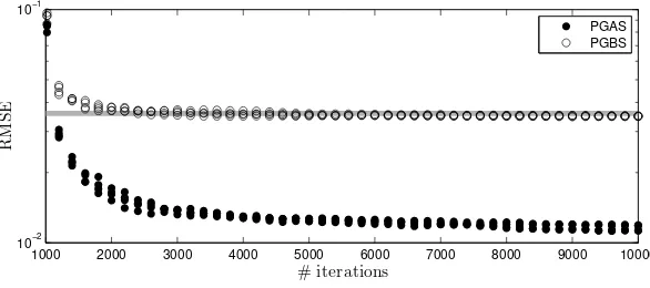
1000 2000 3000 4000 5000 6000 7000 8000 9000 10000
10−2
10−1
# iterations
R
M
S
E
PGAS PGBS
Figure 5: Running RMSEs for x1:T for five independent runs of PGAS (•) and PGBS (◦),
respectively. The truncation level is set to`= 1. The thick gray line corresponds to a run of an untruncated FFBS particle smoother.
Q = R = 0.1. For simplicity, we assume that the system parameters are known and seek the joint smoothing distribution p(x1:T | y1:T). In the non-Markovian formulation
it is possible to apply backward-simulation-based methods, such as PGAS and PGBS, as described in Section 6.2. The problem, however, is that the non-Markovianity gives rise to an O(T2) computational complexity. To obtain more practical inference algorithms we employ the weight truncation strategy (23).
First, we consider the coarse approximation`= 1. We run PGAS and PGBS, both with N = 5 particles for 10 000 iterations (with the first 1 000 discarded as burn-in). We then compute running means of the latent variablesx1:T and, from these, we compute the running
root-mean-squared errors (RMSEs)nrelative to the true posterior means (computed with
a modified Bryson-Frazier smoother, Bierman, 1973). Hence, if no approximation would have been made, we would expectn→0, so any static error can be seen as the effect of the
truncation. The results for five independent runs are shown in Figure 5. First, we note that both methods give accurate results. Still, the error for PGAS is significantly lower than for PGBS. For further comparison, we also run an untruncated forward filter/backward simulator (FFBS) particle smoother (Godsill et al., 2004), using N = 10 000 particles and M = 1 000 backward trajectories, with a computational cost of O(N M T2). The resulting
RMSE value is shown as a thick gray line in Figure 5. This result suggest that PGAS can be a serious competitor to more “classical” particle smoothers, even when there are no unknown parameters of the model. Already with`= 1, PGAS outperforms FFBS in terms of accuracy and, due to the fact that AS allows us to use as few asN = 5 particles at each iteration, at a much lower computational cost.
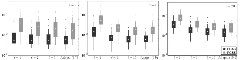
10−3
10−2
10−1
ℓ= 1 ℓ= 2 ℓ= 3 Adapt. (3.7) d= 2
10−3
10−2
10−1
ℓ= 1 ℓ= 5 ℓ= 10 Adapt. (5.9)
d= 5
10−3 10−2 10−1
ℓ= 1 ℓ= 5 ℓ= 10 Adapt. (10.6)
d= 20
PGAS PGBS
Figure 6: Box plots of the RMSE errors for PGAS (black) and PGBS (gray), for 150 ran-dom systems of different dimensionsd(left,d= 2; middle,d= 5; right,d= 20). Different values for the truncation level ` are considered. The rightmost boxes correspond to an adaptive truncation and the values in parentheses are the aver-age truncation levels over all systems and MCMC iterations (the same for both methods). The dots within the boxes show the median errors.
well as an adaptive level with υ = 0.1 and τ = 10−2 (see Section 6.2). All other settings are as above.
Again, we compute the posterior means of x1:T (discarding 1 000 samples) and RMSE
values relative to the true posterior mean. Box plots over the different systems are shown in Figure 6. Since the process noise only enters on one of the state components, the mixing tends to deteriorate as we increase the model order. Figure 3 shows how the probability distributions on{1, . . . , N}change as we increase the truncation level, in two representative cases for a 5th and a 20th order system, respectively. By using an adaptive level, we can obtain accurate results for systems of different dimensions, without having to change any settings between the runs.
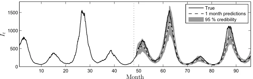
7.3 Epidemiological Model
As a final numerical illustration, we consider identification of an epidemiological model using PGAS. Seasonal influenza epidemics each year cause millions of severe illnesses and hundreds of thousands of deaths world-wide (Ginsberg et al., 2009). Furthermore, new strains of influenza viruses can possibly cause pandemics with very severe effects on the public health. The ability to accurately predict disease activity can enable early response to such epidemics, which in turn can reduce their impact.
We consider a susceptible/infected/recovered (SIR) model with environmental noise and seasonal fluctuations (Keeling and Rohani, 2007; Rasmussen et al., 2011). The model, spec-ified by a stochastic differential equation, is discretized according to the Euler-Maruyama method, yielding
St+dt =St+µPdt−µStdt−(1 +F vt)βtStP−1Itdt, (26a)
It+dt =It−(γ+µ)Itdt+ (1 +F vt)βtStP−1Itdt, (26b)