An Emphatic Approach to the Problem of Off-policy Temporal-Difference Learning

Journal of Machine Learning Research 17 (2016) 1-29 Submitted 11/14; Revised 11/15; Published 5/16

An Emphatic Approach to the Problem

of Off-policy Temporal-Difference Learning

Richard S. Sutton [email protected]

A. Rupam Mahmood [email protected]

Martha White [email protected]

Reinforcement Learning and Artificial Intelligence Laboratory Department of Computing Science, University of Alberta Edmonton, Alberta, Canada T6G 2E8

Editor:Shie Mannor

Abstract

In this paper we introduce the idea of improving the performance of parametric temporal-difference (TD) learning algorithms by selectively emphasizing or de-emphasizing their updates on different time steps. In particular, we show that varying the emphasis of linear TD(λ)’s updates in a particular way causes its expected update to become stable under off-policy training. The only prior model-free TD methods to achieve this with per-step computation linear in the number of function approximation parameters are the gradient-TD family of methods including gradient-TDC, Ggradient-TD(λ), and GQ(λ). Compared to these methods, ouremphatic TD(λ)is simpler and easier to use; it has only one learned parameter vector and one step-size parameter. Our treatment includes general state-dependent discount-ing and bootstrappdiscount-ing functions, and a way of specifydiscount-ing varydiscount-ing degrees of interest in accurately valuing different states.

Keywords: Temporal-difference learning, Off-policy learning, Function approximation, Stability, Convergence.

1. Parametric Temporal-Difference Learning

Temporal-difference (TD) learning is perhaps the most important idea to come out of the field of reinforcement learning. The problem it solves is that of efficiently learning to make a sequence of long-term predictions about how a dynamical system will evolve over time. The key idea is to use the change (temporal difference) from one prediction to the next as an error in the earlier prediction. For example, if you are predicting on each day what the stock-market index will be at the end of the year, and events lead you one day to make a much lower prediction, then a TD method would infer that the predictions made prior to the drop were probably too high; it would adjust the parameters of its prediction function so as to make lower predictions for similar situations in the future. This approach contrasts with conventional approaches to prediction, which wait until the end of the year when the final stock-market index is known before adjusting any parameters, or else make only short-term (e.g., one-day) predictions and then iterate them to produce a year-end prediction. The TD approach is more convenient computationally because it requires less memory and because its computations are spread out uniformly over the year (rather than being bunched

c

together all at the end of the year). A less obvious advantage of the TD approach is that it often produces statistically more accurate answers than conventional approaches (Sutton 1988).

Parametric temporal-difference learning was first studied as the key “learning by gen-eralization” algorithm in Samuel’s (1959) checker player. Sutton (1988) introduced the TD(λ) algorithm and proved convergence in the mean of episodic linear TD(0), the simplest parametric TD method. The potential power of parametric TD learning was convincingly demonstrated by Tesauro (1992, 1995) when he applied TD(λ) combined with neural net-works and self play to obtain ultimately the world’s best backgammon player. Dayan (1992) proved convergence in expected value of episodic linear TD(λ) for allλ_∈[0,1], and Tsitsik-lis and Van Roy (1997) proved convergence with probability one of discounted continuing linear TD(λ). Watkins (1989) extended TD learning to control in the form of Q-learning and proved its convergence in the tabular case (without function approximation, Watkins & Dayan 1992), while Rummery (1995) extended TD learning to control in an on-policy form as the Sarsa(λ) algorithm. Bradtke and Barto (1996), Boyan (1999), and Nedic and Bertsekas (2003) extended linear TD learning to a least-squares form called LSTD(λ). Para-metric TD methods have also been developed as models of animal learning (e.g., Sutton & Barto 1990, Klopf 1988, Ludvig, Sutton & Kehoe 2012) and as models of the brain’s reward systems (Schultz, Dayan & Montague 1997), where they have been particularly influential (e.g., Niv & Schoenbaum 2008, O’Doherty 2012). Sutton (2009, 2012) has suggested that parametric TD methods could be key not just to learning about reward, but to the learning of world knowledge generally, and to perceptual learning. Extensive analysis of parametric TD learning as stochastic approximation is provided by Bertsekas (2012, Chapter 6) and Bertsekas and Tsitsiklis (1996).

Within reinforcement learning, TD learning is typically used to learn approximations to the value function of a Markov decision process (MDP). Here the value of a state s, denoted vπ(s), is defined as the sum of the expected long-term discounted rewards that

will be received if the process starts insand subsequently takes actions as specified by the decision-making policy π, called the target policy. If there are a small number of states, then it may be practical to approximate the function vπ by a table, but more generally

a parametric form is used, such as a polynomial, multi-layer neural network, or linear mapping. Also key is the source of the data, in particular, the policy used to interact with the MDP. If the data is obtained while following the target policyπ, then good convergence results are available for linear function approximation. This case is calledon-policy learning because learning occurs while “on” the policy being learned about. In the alternative, off-policy case, one seeks to learn about vπ while behaving (selecting actions) according to

a different policy called the behavior policy, which we denote by µ. Baird (1995) showed definitively that parametric TD learning was much less robust in the off-policy case (for

An Emphatic Approach to Off-policy TD Learning

Over the years, several different approaches have been taken to solving the problem of off-policy learning with TD learning (λ < 1). Baird (1995) proposed an approach based on gradient descent in the Bellman error for general parametric function approximation that has the desired computational properties, but which requires access to the MDP for double sampling and which in practice often learns slowly. Gordon (1995, 1996) proposed restricting attention to function approximators that are averagers, but this does not seem to be possible without storing many of the training examples, which would defeat the primary strength that we seek to obtain from parametric function approximation. The LSTD(λ) method was always relatively robust to off-policy training (e.g., Lagoudakis & Parr 2003, Yu 2010, Mahmood, van Hasselt & Sutton 2014), but its per-step computational complexity is quadratic in the number of parameters of the function approximator, as opposed to the linear complexity of TD(λ) and the other methods. Perhaps the most successful approach to date is the gradient-TD approach (e.g., Maei 2011, Sutton et al. 2009, Maei et al. 2010), including hybrid methods such as HTD (Hackman 2012). Gradient-TD methods are of linear complexity and guaranteed to converge for appropriately chosen step-size parameters but are more complex than TD(λ) because they require a second auxiliary set of parameters with a second step size that must be set in a problem-dependent way for good performance. The studies by White (2015), Geist and Scherrer (2014), and Dann, Neumann, and Peters (2014) are the most extensive empirical explorations of gradient-TD and related methods to date.

In this paper we explore a new approach to solving the problem of off-policy TD learning with function approximation. The approach has novel elements but is similar to that devel-oped by Precup, Sutton, and Dasgupta in 2001. They proposed to use importance sampling to reweight the updates of linear TD(λ), emphasizing or de-emphasizing states as they were encountered, and thereby create a weighting equivalent to the stationary distribution under the target policy, from which the results of Tsitsiklis and Van Roy (1997) would apply and guarantee convergence. As we discuss later, this approach has very high variance and was eventually abandoned in favor of the gradient-TD approach. The new approach we explore in this paper is similar in that it also varies emphasis so as to reweight the distribution of linear TD(λ) updates, but to a different goal. The new goal is to create a weighting equiva-lent to thefollowon distribution for the target policy started in the stationary distribution of the behavior policy. The followon distribution weights states according to how often they would occur prior to termination by discounting if the target policy was followed.

Our main result is to prove that varying emphasis according to the followon distribution produces a new version of linear TD(λ),called emphatic TD(λ), that is stable under general off-policy training. By “stable” we mean that the expected update over the ergodic distri-bution (Tsitsiklis & Van Roy 1997) is a contraction, involving a positive definite matrix. We concentrate on stability in this paper because it is a prerequisite for full convergence of the stochastic algorithm. Demonstrations that the linear TD(λ) is not stable under off-policy training have been the focus of previous counterexamples (Baird 1995, Tsitsiklis & Van Roy 1996, 1997, see Sutton & Barto 1998). Substantial additional theoretical machinery would be required for a full convergence proof. Recent work by Yu (2015a,b) builds on our stability result to prove that the emphatic TD(λ) converges with probability one.

In this paper we first treat the simplest algorithm for which the difficulties of off-policy temporal-difference (TD) learning arise—the TD(0) algorithm with linear function

imation. We examine the conditions under which the expected update of on-policy TD(0) is stable, then why those conditions do not apply under off-policy training, and finally how they can be recovered for off-policy training using established importance-sampling methods together with the emphasis idea. After introducing the basic idea of emphatic algorithms using the special case of TD(0), we then develop the general case. In particular, we consider a case with general state-dependent discounting and bootstrapping functions, and with a user-specified allocation of function approximation resources. Our new theoretical results and the emphatic TD(λ) algorithm are presented fully for this general case. Empirical ex-amples elucidating the main theoretical results are presented in the last section prior to the conclusion.

2. On-policy Stability of TD(0)

To begin, let us review the conditions for stability of conventional TD(λ) under on-policy training with data from a continuing finite Markov decision process. Consider the simplest function approximation case, that of linear TD(λ) with λ = 0 and constant discount-rate parameter γ ∈ [0,1). Conventional linear TD(0) is defined by the following update to the parameter vector θt ∈ Rn, made at each of a sequence of time steps t = 0,1,2, . . ., on

transition from state St∈ Sto state St+1 ∈S, taking action At∈A and receiving reward

Rt+1 ∈R:

θt+1 =. θt+α

Rt+1+γθt>φ(St+1)−θ>t φ(St)

φ(St), (1)

whereα >0 is a step-size parameter, andφ(s)∈Rn _{is the feature vector corresponding to}

states. The notation “=” indicates an equality by definition rather than one that follows. from previous definitions. In on-policy training, the actions are chosen according to a target policyπ:A_×S_→[0,1], whereπ(a_|s)=. _P{At=a|St=s}. The state and action setsSandA

are assumed to be finite, but the number of states is assumed much larger than the number of learned parameters, _|S_|=. N n, so that function approximation is necessary. We use linear function approximation, in which the inner product of the parameter vector and the feature vector for a state is meant to be an approximation to the value of that state:

θ>_t φ(s)_≈vπ(s)=. Eπ[Gt|St=s], (2)

whereEπ[·] denotes an expectation conditional on all actions being selected according to π,

and Gt, thereturn at timet, is defined by

Gt=. Rt+1+γRt+2+γ2Rt+3+· · · . (3)

The TD(0) update (1) can be rewritten to make the stability issues more transparent:

θt+1=θt+α

Rt+1φ(St)

| {z }

bt∈Rn

−φ(St) (φ(St)−γφ(St+1))>

| {z }

At∈Rn×n

θt

=θt+α(bt−Atθt) (4)

An Emphatic Approach to Off-policy TD Learning

The matrix At multiplies the parameter θt and is thereby critical to the stability of the

iteration. To develop intuition, consider the special case in which At is a diagonal matrix.

If any of the diagonal elements are negative, then the corresponding diagonal element of I₋αAt will be greater than one, and the corresponding component ofθt will be amplified,

which will lead to divergence if continued. (The second term (αbt) does not affect the

stability of the iteration.) On the other hand, if the diagonal elements ofAtare all positive,

thenαcan be chosen smaller than one over the largest of them, such thatI₋αAtis diagonal

with all diagonal elements between 0 and 1. In this case the first term of the update tends to shrinkθt, and stability is assured. In general,θt will be reduced toward zero whenever

At is positive definite.1

In actuality, however, At and bt are random variables that vary from step to step,

in which case stability is determined by the steady-state expectation, limt→∞E[At]. In

our setting, after an initial transient, states will be visited according to the steady-state distribution underπ (which we assume exists). We represent this distribution by a vector dπ, each component of which gives the limiting probability of being in a particular state2

[dπ]s=. dπ(s)= lim. t→∞P{St=s}, which we assume exists and is positive at all states (any

states not visited with nonzero probability can be removed from the problem). The special property of the steady-state distribution is that once the process is in it, it remains in it. Let Pπ denote the N ×N matrix of transition probabilities [Pπ]ij =. Paπ(a|i)p(j|i, a) where

p(j_|i, a)=. _P{St+1=j|St=i, At=a}. Then the special property of dπ is that

P>_πdπ =dπ. (5)

Consider any stochastic algorithm of the form (4), and let A = lim. t→∞E[At] and

b = lim. t→∞E[bt]. We define the stochastic algorithm to be stable if and only if the

corresponding deterministic algorithm, ¯

θt+1= ¯. θt+α(b−Aθ¯t), (6)

is convergent to a unique fixed point independent of the initial ¯θ0. This will occur iff the

A matrix has a full set of eigenvalues all of whose real parts are positive. If a stochastic algorithm is stable andαis reduced according to an appropriate schedule, then its parameter vector may converge with probability one. However, in this paper we focus only on stability as a prerequisite for convergence (of the original stochastic algorithm), leaving convergence itself to future work. If the stochastic algorithm converges, it is to a fixed point ¯θ of the deterministic algorithm, at which Aθ¯= b, or ¯θ = A−1b. (Stability assures existence of the inverse.) In this paper we focus on establishing stability by proving thatA is positive definite. From definiteness it immediately follows that A has a full set of eigenvectors (because y>Ay>0,∀y6=0) and that the corresponding eigenvalues all have real parts.3

1. A real matrixAis defined to bepositive definite in this paper iffy>Ay>0 for any real vectory6=0. 2. Here and throughout the paper we use brackets with subscripts to denote the individual elements of

vectors and matrices.

3. To see the latter, let Re(x) denote the real part of a complex numberx, and lety∗denotes the conjugate transpose of a complex vector y. Then, for any eigenvalue–eigenvector pair λ,y: 0 < Re(y∗Ay) = Re(y∗λy) = Re(λ)y∗y =⇒ 0<Re(λ).

Now let us return to analyzing on-policy TD(0). Its Amatrix is A= lim

t→∞E[At] = limt→∞Eπ

h

φ(St) (φ(St)−γφ(St+1))>

i

=X

s

dπ(s)φ(s) φ(s)−γ

X

s0

[Pπ]ss0φ(s0)

!>

=Φ>Dπ(I−γPπ)Φ,

where Φ is the N _×n matrix with the φ(s) as its rows, and Dπ is the N ×N diagonal

matrix withdπ on its diagonal. ThisAmatrix is typical of those we consider in this paper

in that it consists of Φ> and Φ wrapped around a distinctive N _×N matrix that varies with the algorithm and the setting, and which we call thekey matrix. An Amatrix of this form will be positive definite whenever the corresponding key matrix is positive definite.4 In this case the key matrix isDπ(I−γPπ).

For a key matrix of this type, positive definiteness is assured if all of its columns sum to nonnegative numbers. This was shown by Sutton (1988, p. 27) based on two previously established theorems. One theorem says that any matrixMis positive definite if and only if the symmetric matrixS=M+M>is positive definite (Sutton 1988, appendix). The second theorem says that any symmetric real matrixS is positive definite if the absolute values of its diagonal entries are greater than the sum of the absolute values of the corresponding off-diagonal entries (Varga 1962, p. 23). For our key matrix, Dπ(I−γPπ), the diagonal

entries are positive and the off-diagonal entries are negative, so all we have to show is that each row sum plus the corresponding column sum is positive. The row sums are all positive becausePπ is a stochastic matrix andγ <1. Thus it only remains to show that the column

sums are nonnegative.

Note that the row vector of the column sums of any matrix Mcan be written as 1>M, where1 is the column vector with all components equal to 1. The column sums of our key matrix, then, are:

1>Dπ(I−γPπ) =d>π(I−γPπ)

=d>_{π −}γd>_πPπ

=d>_{π −}γd>_π (by (5)) = (1₋γ)dπ,

all components of which are positive. Thus, the key matrix and its A matrix are positive definite, and on-policy TD(0) is stable. Additional conditions and a schedule for reducing

α over time (as in Tsitsiklis and Van Roy 1997) are needed to prove convergence with probability one, θ_∞ = A−1b, but the analysis above includes the most important steps that vary from algorithm to algorithm.

An Emphatic Approach to Off-policy TD Learning

3. Instability of Off-policy TD(0)

Before developing the off-policy setting in detail, it is useful to understand informally why TD(0) is susceptible to instability. TD learning involves learning an estimate from an es-timate, which can be problematic if there is generalization between the two estimates. For example, suppose there is a transition between two states with the same feature represen-tation except that the second is twice as big:

0

The other two goals for approximation are related to the

Bellman equation

, which can

be written compactly in vector form as

v

⇡

=

B

⇡

v

⇡

,

(7)

where

B

⇡

:

R

|S|

!

R

|S|

is the

Bellman operator

for policy

⇡

, defined by

(

B

⇡

v

)(

s

) =

X

a2A

⇡

(

s, a

)

"

r

(

s, a

) +

X

s0_2S

p

(

s

0

|

s, a

)

v

(

s

0

)

#

,

8

s

2 S

,

8

v

:

S !

R

.

(8)

(If the state and action spaces are continuous, then the sums are replaced by integrals and

the function

p

(

·|

s, a

) is taken to be a probability density.) The true value function

v

⇡

is

the unique solution to the Bellman equation; the Bellman equation can be viewed as an

alternate way of defining

v

⇡

. For any value function

v

:

S !

R

not equal to

v

⇡

, there will

always be at least one state

s

at which

v

(

s

)

₆

= (

B

⇡

v

)(

s

).

The discrepancy between the two sides of the Bellman equation,

v

⇡

B

⇡

v

⇡

, is an error

vector, and reducing it is the basis for our second and third goals for approximation. The

second goal is to minimize the error vector’s length in the

d

-metric. That is, to minimize

the mean-squared

Bellman error

:

BE(

✓

) =

X

s2S

d

(

s

)

⇥

(

B

⇡

v

✓

)(

s

)

v

✓

(

s

)

⇤

2

.

(9)

Note that if

v

⇡

is not representable, then it is not be possible to reduce the Bellman error

to zero. For any

v

✓

, the corresponding

B

⇡

v

✓

will generally not be representable; it will lie

outside the space of representable functions, as suggested by the figure...

Finally, in our third goal of approximation, we first project the Bellman error and then

minimize its length. That is, we minimize the error not in the Bellman equation (7) but in

its projected form:

v

✓

= ⇧

B

⇡

v

✓

,

(10)

Unlike the original Bellman equation, for most function approximators (e.g., linear ones)

the projected Bellman equation can be solved exactly. If it can’t be solved exactly, you can

minimize the mean-squared

projected Bellman error

:

PBE(

✓

) =

X

s2S

d

(

s

)

⇥

(⇧(

B

⇡

v

✓

v

✓

))(

s

)

⇤

2

.

(11)

The minimum is achieved at the

projection fixpoint

, at which

X

s2S

d

(

s

)

⇥

(

B

⇡

v

✓

)(

s

)

v

✓

(

s

)

⇤

r

✓

v

✓

(

s

) =

~

0

.

(12)

PBE = 0

min BE

✓

1

✓

2

Now we must finish this section by discussing the relative merits of the second and

third goals. This comes down to two counterexamples using POMDPs. One shows that

the BE is not well defined for POMDP data, the other shows that the minimum is not

5

When approximate DP converges, it converges to a value function at which the PBE

(12) is zero and, of course, to a fixpoint of its update (14).

That approximate DP converges to a zero of the PBE for linear FA and the on-policy

distribution is an important positive result, representing the most successful generalization

of DP to a powerful class of function approximators. It was a breakthrough of sorts,

representing significant progress towards addressing Bellman’s “curse of dimensionality.”

However, linearity and the on-policy distribution remained significant limitations. In this

paper we will present methods that remove both limitations, so let us examine them more

carefully.

The status of approximate DP’s limitation to linear function approximators is not

com-pletely clear. In practice, such algorithms have been widely used with nonlinear function

approximators with good results. Tesauro’s (1992, 1995) celebrated results with

backgam-mon, for example, were obtained with a nonlinear neural-network function approximator.

It is in fact extremely difficult to construct a example in which approximate DP fails to

converge under the on-policy distribution. The only such counterexample currently known

is Tsitsiklis and Van Roy’s spiral example, which is complex and contrived. We have tried

to construct a simpler one without success. Moreover, we have recently shown that even,

in the nonlinear case, all fixpoints of the approximate DP update are stable—that if the

approximator is started near a fixpoint it will converge to it (Maei, Sutton & Van Roy

in preparation). It seems quite likely to us that there could be a significant further

posi-tive result to be obtained for nonlinear function approximators and approximate DP. For

the moment, however, there are no positive theoretical results for approximate DP and

nonlinear function approximators.

Approximate DP’s limitation to the on-policy distribution appears more fundamental.

Simple counterexamples were presented by Baird (1995) and by Tsitsiklis and Van Roy

(1997) who also developed a theoretical understanding of the instability. Perhaps the

sim-plest counterexample, and a good one for understanding the issues, is given by this fragment

of an MDP:

0

The other two goals for approximation are related to the

Bellman equation

, which can

be written compactly in vector form as

v

_⇡

=

B

_⇡

v

_⇡

,

(7)

where

B

_⇡

:

R

|S|

_!

R

|S|

is the

Bellman operator

for policy

⇡

, defined by

(

B

_⇡

v

)(

s

) =

X

a

_2A

⇡

(

s, a

)

"

r

(

s, a

) +

X

s

0

_2S

p

(

s

0

_|

s, a

)

v

(

s

0

)

#

,

₈

s

_{2 S}

,

₈

v

:

_{S !}

R

.

(8)

(If the state and action spaces are continuous, then the sums are replaced by integrals and

the function

p

(

·|

s, a

) is taken to be a probability density.) The true value function

v

_⇡

is

the unique solution to the Bellman equation; the Bellman equation can be viewed as an

alternate way of defining

v

_⇡

. For any value function

v

:

_{S !}

R

not equal to

v

_⇡

, there will

always be at least one state

s

at which

v

(

s

) = (

B

_⇡

v

)(

s

).

The discrepancy between the two sides of the Bellman equation,

v

_⇡

B

_⇡

v

_⇡

, is an error

vector, and reducing it is the basis for our second and third goals for approximation. The

second goal is to minimize the error vector’s length in the

d

-metric. That is, to minimize

the mean-squared

Bellman error

:

BE(

✓

) =

X

s

_2S

d

(

s

)

⇥

(

B

_⇡

v

_✓

)(

s

)

v

_✓

(

s

)

⇤

2

.

(9)

Note that if

v

_⇡

is not representable, then it is not be possible to reduce the Bellman error

to zero. For any

v

_✓

, the corresponding

B

_⇡

v

_✓

will generally not be representable; it will lie

outside the space of representable functions, as suggested by the figure...

Finally, in our third goal of approximation, we first project the Bellman error and then

minimize its length. That is, we minimize the error not in the Bellman equation (7) but in

its projected form:

v

_✓

= ⇧

B

_⇡

v

_✓

,

(10)

Unlike the original Bellman equation, for most function approximators (e.g., linear ones)

the projected Bellman equation can be solved exactly. If it can’t be solved exactly, you can

minimize the mean-squared

projected Bellman error

:

PBE(

✓

) =

X

s

_2S

d

(

s

)

⇥

(⇧(

B

_⇡

v

_✓

v

_✓

))(

s

)

⇤

2

.

(11)

The minimum is achieved at the

projection fixpoint

, at which

X

s

_2S

d

(

s

)

⇥

(

B

_⇡

v

_✓

)(

s

)

v

_✓

(

s

)

⇤

_r

_✓

v

_✓

(

s

) =

~

0

.

(12)

PBE = 0

min BE

✓

₁

✓

₂

Now we must finish this section by discussing the relative merits of the second and

third goals. This comes down to two counterexamples using POMDPs. One shows that

the BE is not well defined for POMDP data, the other shows that the minimum is not

5

2

✓

So we see there is a fundamental sense in which DP does not work well with parametric

function approximation. This is the problem of DP and FA.

There is a special case that works, where the states are updated with the on-policy

distribution.

✓

t+1

=

✓

t

+

↵

X

s

d

⇡

(

s

)

⇥

(

B

⇡

v

✓t

)(

s

)

v

✓t

(

s

)

⇤

r

✓t

v

✓t

(

s

)

,

(16)

12 where hereθand 2θare the estimated values of the two states—that is, their feature repre-sentations are a single feature that is 1 for the first state and 2 for the second (cf. Tsitsiklis & Van Roy 1996). Now suppose that θ is 10 and the reward on the transition is 0. The transition is then from a state valued at 10 to a state valued at 20. If γ is near 1 andα

is 0.1, then θwill be increased to approximately 11. But then the next time the transition occurs there will be an even bigger increase in value, from 11 to 22, and a bigger increase in

θ, to approximately 12.1. If this transition is experienced repeatedly on its own, then the system is unstable and the parameter increases without bound—it diverges. We call this theθ_→2θproblem.

In on-policy learning, repeatedly experiencing just this single problematic transition cannot happen, because, after the highly-valued 2θ state has been entered, it must then be exited. The transition from it will either be to a lesser or equally-valued state, in which case θwill be significantly decreased, or to an even higher-valued state which in turn must be followed by an even larger decrease in its estimated value or a still higher-valued state. Eventually, the promise of high value must be made good in the form of a high reward, or else estimates will be decreased, and this ultimately constrains θ and forces stability and convergence. In the off-policy case, however, if there is a deviation from the target policy then the promise is excused and need never be fulfilled. Later in this section we present a complete example of how the θ_→2θ problem can cause instability and divergence under off-policy training.

With these intuitions, we now detail our off-policy setting. As in the on-policy case, the data is a single, infinite-length trajectory of actions, rewards, and feature vectors generated by a continuing finite Markov decision process. The difference is that the actions are selected not according to the target policy π, but according to a different behavior policy

µ:A_×S_→[0,1], yet still we seek to estimate state values under π (as in (2)). Of course, it would be impossible to estimate the values under π if the actions that π would take were never taken byµ and their consequences were never observed. Thus we assume that

µ(a|s) >0 for every state and action for which π(a|s) >0. This is called the assumption of coverage. It is trivially satisfied by any -greedy or soft behavior policy. As before we assume that there is a stationary distribution dµ(s) = lim. t→∞P{St=s} >0,∀s∈ S, with

correspondingN-vector dµ.

Even if there is coverage, the behavior policy will choose actions with proportions dif-ferent from the target policy. For example, some actions taken byµmight never be chosen byπ. To address this, we use importance sampling to correct for the relative probability of taking the action actually taken,At, in the state actually encountered,St, under the target

and behavior policies:

ρt=.

π(At|St)

µ(At|St)

.

This quantity is called the importance sampling ratio at time t. Note that its expected value is one:

Eµ[ρt|St=s] =

X

a

µ(a|s)π(a|s)

µ(a|s) =

X

a

π(a|s) = 1.

The ratio will be exactly one only on time steps on which the action probabilities for the two policies are exactly the same; these time steps can be treated the same as in the on-policy case. On other time steps the ratio will be greater or less than one depending on whether the action taken was more or less likely under the target policy than under the behavior policy, and some kind of correction is needed.

In general, for any random variable Zt+1 dependent on St,At andSt+1, we can recover

its expectation under the target policy by multiplying by the importance sampling ratio:

Eµ[ρtZt+1|St=s] =

X

a

µ(a_|s)π(a|s)

µ(a_|s)Zt+1 =X

a

π(a|s)Zt+1

=_Eπ[Zt+1|St=s], ∀s∈S. (7)

We can use this fact to begin to adapt TD(0) for off-policy learning (Precup, Sutton & Singh 2000). We simply multiply the whole TD(0) update (1) by ρt:

θt+1 =. θt+ρtα

Rt+1+γθ>t φt+1−θt>φt

φt (8)

=θt+α

ρtRt+1φt

| {z } bt

−ρtφt(φt−γφt+1)>

| {z }

At

θt

,

where here we have used the shorthandφt=. φ(St). Note that if the action taken at timet

is never taken under the target policy in that state, then ρt= 0 and there is no update on

that step, as desired. We call this algorithmoff-policy TD(0). Off-policy TD(0)’s A matrix is

A= lim

t→∞E[At] = limt→∞Eµ

h

ρtφt(φt−γφt+1)>

i

=X

s

dµ(s)Eµ

h

ρkφk(φk−γφk+1)>

Sk=s

i

=X

s

dµ(s)Eπ

h

φk(φk−γφk+1)>

Sk=s

i

(by (7))

=X

s

dµ(s)φ(s) φ(s)−γ

X

s0

[Pπ]ss0φ(s0)

!>

An Emphatic Approach to Off-policy TD Learning

whereDµis theN×N diagonal matrix with the stationary distributiondµon its diagonal.

Thus, the key matrix that must be positive definite is Dµ(I−γPπ) and, unlike in the

on-policy case, the distribution and the transition probabilities do not match. We do not have an analog of (5),P_π>dµ6=dµ, and in fact the column sums may be negative and the matrix

not positive definite, in which case divergence of the parameter is likely.

A simple θ_→2θ example of divergence that fits the setting in this section is shown in Figure 1. From each state there are two actions,leftandright, which take the process to the left or right states. All the rewards are zero. As before, there is a single parameter θ and the single feature is 1 and 2 in the two states such that the approximate values are θ and 2θ as shown. The behavior policy is to go left and right with equal probability from both states, such that equal time is spent on average in both states,dµ= (0.5,0.5)>. The target

policy is to go right in both states. We seek to learn the value from each state given that theright action is continually taken. The transition probability matrix for this example is:

Pπ =

0 1 0 1

.

The key matrix is

Dµ(I−γPπ) =

0.5 0 0 0.5

×

1 ₋0.9 0 0.1

=

0.5 ₋0.45 0 0.05

. (9) We can see an immediate indication that the key matrix may not be positive definite in that the second column sums to a negative number. More definitively, one can show that it is not positive definite by multiplying it on both sides byy=Φ= (1,2)>_:

Φ>Dµ(I−γPπ)Φ=

1 2×

0.5 −0.45 0 0.05

× 1 2

=1 2×

−0.4 0.1

=−0.2.

That this is negative means that the key matrix is not positive definite. We have also calculated here the A matrix; it is this negative scalar, A =₋0.2. Clearly, this expected update and algorithm are not stable.

It is also easy to see the instability of this example more directly, without matrices. We know that only transitions under the right action cause updates, as ρt will be zero for

the others. Assume for concreteness that initially θt = 10 and that α = 0.1. On a right

transition from the first state the update will be

θt+1=θt+ρtα

Rt+1+γθt>φt+1−θ>t φt

φt

= 10 + 2·0.1 (0 + 0.9·10·2−10·1) 1 = 10 + 1.6,

The other two goals for approximation are related to the

Bellman equation

, which can

be written compactly in vector form as

v

_⇡

=

B

_⇡

v

_⇡

,

(7)

where

B

⇡

:

R

|S|

!

R

|S|

is the

Bellman operator

for policy

⇡

, defined by

(

B

⇡

v

)(

s

) =

X

a2A

⇡

(

s, a

)

"

r

(

s, a

) +

X

s0_2S

p

(

s

0

_|

s, a

)

v

(

s

0

)

#

,

₈

s

_{2 S}

,

₈

v

:

_{S !}

R

.

(8)

(If the state and action spaces are continuous, then the sums are replaced by integrals and

the function

p

(

_·|

s, a

) is taken to be a probability density.) The true value function

v

⇡

is

the unique solution to the Bellman equation; the Bellman equation can be viewed as an

alternate way of defining

v

⇡

. For any value function

v

:

S !

R

not equal to

v

⇡

, there will

always be at least one state

s

at which

v

(

s

)

₆

= (

B

⇡

v

)(

s

).

The discrepancy between the two sides of the Bellman equation,

v

⇡

B

⇡

v

⇡

, is an error

vector, and reducing it is the basis for our second and third goals for approximation. The

second goal is to minimize the error vector’s length in the

d

-metric. That is, to minimize

the mean-squared

Bellman error

:

BE(

✓

) =

X

s2S

d

(

s

)

⇥

(

B

⇡

v

✓

)(

s

)

v

✓

(

s

)

⇤

2

.

(9)

Note that if

v

⇡

is not representable, then it is not be possible to reduce the Bellman error

to zero. For any

v

_✓

, the corresponding

B

⇡

v

✓

will generally not be representable; it will lie

outside the space of representable functions, as suggested by the figure...

Finally, in our third goal of approximation, we first project the Bellman error and then

minimize its length. That is, we minimize the error not in the Bellman equation (7) but in

its projected form:

v

✓

= ⇧

B

⇡

v

✓

,

(10)

Unlike the original Bellman equation, for most function approximators (e.g., linear ones)

the projected Bellman equation can be solved exactly. If it can’t be solved exactly, you can

minimize the mean-squared

projected Bellman error

:

PBE(

✓

) =

X

s2S

d

(

s

)

⇥

(⇧(

B

_⇡

v

_✓

v

_✓

))(

s

)

⇤

2

.

(11)

The minimum is achieved at the

projection fixpoint

, at which

X

s2S

d

(

s

)

⇥

(

B

_⇡

v

_✓

)(

s

)

v

_✓

(

s

)

⇤

_r

_✓

v

_✓

(

s

) =

~

0

.

(12)

PBE = 0

min BE

✓

1

✓

2

Now we must finish this section by discussing the relative merits of the second and

third goals. This comes down to two counterexamples using POMDPs. One shows that

the BE is not well defined for POMDP data, the other shows that the minimum is not

5

= 0.9

= 0 µ(right_|·) = 0.5

⇡(right|·) = 1

When approximate DP converges, it converges to a value function at which the PBE

(12) is zero and, of course, to a fixpoint of its update (14).

That approximate DP converges to a zero of the PBE for linear FA and the on-policy

distribution is an important positive result, representing the most successful generalization

of DP to a powerful class of function approximators. It was a breakthrough of sorts,

representing significant progress towards addressing Bellman’s “curse of dimensionality.”

However, linearity and the on-policy distribution remained significant limitations. In this

paper we will present methods that remove both limitations, so let us examine them more

carefully.

The status of approximate DP’s limitation to linear function approximators is not

com-pletely clear. In practice, such algorithms have been widely used with nonlinear function

approximators with good results. Tesauro’s (1992, 1995) celebrated results with

backgam-mon, for example, were obtained with a nonlinear neural-network function approximator.

It is in fact extremely difficult to construct a example in which approximate DP fails to

converge under the on-policy distribution. The only such counterexample currently known

is Tsitsiklis and Van Roy’s spiral example, which is complex and contrived. We have tried

to construct a simpler one without success. Moreover, we have recently shown that even,

in the nonlinear case, all fixpoints of the approximate DP update are stable—that if the

approximator is started near a fixpoint it will converge to it (Maei, Sutton & Van Roy

in preparation). It seems quite likely to us that there could be a significant further

posi-tive result to be obtained for nonlinear function approximators and approximate DP. For

the moment, however, there are no positive theoretical results for approximate DP and

nonlinear function approximators.

Approximate DP’s limitation to the on-policy distribution appears more fundamental.

Simple counterexamples were presented by Baird (1995) and by Tsitsiklis and Van Roy

(1997) who also developed a theoretical understanding of the instability. Perhaps the

sim-plest counterexample, and a good one for understanding the issues, is given by this fragment

of an MDP:

0

The other two goals for approximation are related to the

Bellman equation

, which can

be written compactly in vector form as

v

_⇡

=

B

_⇡

v

_⇡

,

(7)

where

B

_⇡

:

R

|S|

_!

R

|S|

is the

Bellman operator

for policy

⇡

, defined by

(

B

_⇡

v

)(

s

) =

X

a

_2A

⇡

(

s, a

)

"

r

(

s, a

) +

X

s

0

2S

p

(

s

0

|

s, a

)

v

(

s

0

)

#

,

8

s

2 S

,

8

v

:

S !

R

.

(8)

(If the state and action spaces are continuous, then the sums are replaced by integrals and

the function

p

(

·|

s, a

) is taken to be a probability density.) The true value function

v

_⇡

is

the unique solution to the Bellman equation; the Bellman equation can be viewed as an

alternate way of defining

v

_⇡

. For any value function

v

:

S !

R

not equal to

v

_⇡

, there will

always be at least one state

s

at which

v

(

s

) = (

B

_⇡

v

)(

s

).

The discrepancy between the two sides of the Bellman equation,

v

_⇡

B

_⇡

v

_⇡

, is an error

vector, and reducing it is the basis for our second and third goals for approximation. The

second goal is to minimize the error vector’s length in the

d

-metric. That is, to minimize

the mean-squared

Bellman error

:

BE(

✓

) =

X

s

_2S

d

(

s

)

⇥

(

B

_⇡

v

_✓

)(

s

)

v

_✓

(

s

)

⇤

2

.

(9)

Note that if

v

_⇡

is not representable, then it is not be possible to reduce the Bellman error

to zero. For any

v

_✓

, the corresponding

B

_⇡

v

_✓

will generally not be representable; it will lie

outside the space of representable functions, as suggested by the figure...

Finally, in our third goal of approximation, we first project the Bellman error and then

minimize its length. That is, we minimize the error not in the Bellman equation (7) but in

its projected form:

v

_✓

= ⇧

B

_⇡

v

_✓

,

(10)

Unlike the original Bellman equation, for most function approximators (e.g., linear ones)

the projected Bellman equation can be solved exactly. If it can’t be solved exactly, you can

minimize the mean-squared

projected Bellman error

:

PBE(

✓

) =

X

s

_2S

d

(

s

)

⇥

(⇧(

B

_⇡

v

_✓

v

_✓

))(

s

)

⇤

2

.

(11)

The minimum is achieved at the

projection fixpoint

, at which

X

s

_2S

d

(

s

)

⇥

(

B

_⇡

v

_✓

)(

s

)

v

_✓

(

s

)

⇤

r

_✓

v

_✓

(

s

) =

~

0

.

(12)

PBE = 0

min BE

✓

₁

✓

₂

Now we must finish this section by discussing the relative merits of the second and

third goals. This comes down to two counterexamples using POMDPs. One shows that

the BE is not well defined for POMDP data, the other shows that the minimum is not

5

2

✓

So we see there is a fundamental sense in which DP does not work well with parametric

function approximation. This is the problem of DP and FA.

There is a special case that works, where the states are updated with the on-policy

distribution.

✓

t+1

=

✓

t

+

↵

X

s

d

⇡

(

s

)

⇥

(

B

⇡

v

✓t

)(

s

)

v

✓t

(

s

)

⇤

r

✓t

v

✓t

(

s

)

,

(16)

12

Figure 1: θ→2θexample without a terminal state.

whereas, on a righttransition from the second state the update will be

θt+1=θt+ρtα

Rt+1+γθt>φt+1−θ>t φt

φt

= 10 + 2_·0.1 (0 + 0.9_·10_·2₋10_·2) 2 = 10₋0.8.

These two transitions occur equally often, so the net change will be positive. That is,θwill increase, moving farther from its correct value, zero. Everything is linear in θ, so the next time around, with a larger starting θ, the increase in θ will be larger still, and divergence occurs. A smaller value ofα would not prevent divergence, only reduce its rate.

4. Off-policy Stability of Emphatic TD(0)

The deep reason for the difficulty of off-policy learning is that the behavior policy may take the process to a distribution of states different from that which would be encountered under the target policy, yet the states might appear to be the same or similar because of function approximation. Earlier work by Precup, Sutton and Dasgupta (2001) attempted to completely correct for the different state distribution using importance sampling ratios to reweight the states encountered. It is theoretically possible to convert the state weighting from dµ to dπ using the product of all importance sampling ratios from time 0, but in

practice this approach has extremely high variance and is infeasible for the continuing (non-episodic) case. It works in theory because after converting the weighting the key matrix is Dπ(I−γPπ) again, which we know to be positive definite.

Most subsequent works abandoned the idea of completely correcting for the state dis-tribution. For example, the work on gradient-TD methods (e.g., Sutton et al. 2009, Maei 2011) seeks to minimize the mean-squared projected Bellman error weighted bydµ. We call

this an excursion setting because we can think of the contemplated switch to the target policy as an excursion from the steady-state distribution of the behavior policy,dµ. The

ex-cursions would start fromdµ and then followπ until termination, followed by a resumption

ofµand thus a gradual return todµ. Of course these excursions never actually occur during

off-policy learning, they are just contemplated, and thus the state distribution in fact never leaves dµ. It is the excursion view that we take in this paper, but still we use techniques

similar to those introduced by Precup et al. (2001) to determine an emphasis weighting that corrects for the state distribution, only toward a different goal (see also Kolter 2011).

The excursion notion suggests a different weighting of TD(0) updates. We consider that at every time step we are beginning a new contemplated excursion from the current state. The excursion thus would begin in a state sampled fromdµ. If an excursion started it would

An Emphatic Approach to Off-policy TD Learning

variableFt, defined byF0 = 1 and

Ft=. γρt−1Ft−1+ 1, ∀t >0, (10)

which we call the followon trace. Specifically, we define emphatic TD(0) by the following update:

θt+1 =. θt+αFtρt

Rt+1+γθ>t φt+1−θt>φt

φt (11)

=θt+α

FtρtRt+1φt

| {z }

bt

−Ftρtφt(φt−γφt+1)>

| {z }

At

θt

.

Emphatic TD(0)’s A matrix is A= lim

t→∞E[At] = limt→∞Eµ

h

Ftρtφt(φt−γφt+1)>

i

=X

s

dµ(s) lim t→∞Eµ

h

Ftρtφt(φt−γφt+1)>

St=s

i

=X

s

dµ(s) lim

t→∞Eµ[Ft|St=s]Eµ

h

ρtφt(φt−γφt+1)>

St=s

i

(because, given St,Ft is independent of ρtφt(φt−γφt+1)>)

=X

s

dµ(s) lim

t→∞Eµ[Ft|St=s]

| {z }

f(s)

Eµ

h

ρkφk(φk−γφk+1)>

Sk=s

i

=X

s

f(s)Eπ

h

φk(φk−γφk+1)>

Sk=s

i

(by (7))

=X

s

f(s)φ(s) φ(s)₋γX

s0

[Pπ]ss0φ(s0)

!_>

=Φ>F(I₋γPπ)Φ,

where F is a diagonal matrix with diagonal elements f(s) =. dµ(s) limt→∞Eµ[Ft|St=s],

which we assume exists. As we show later, the vectorf _∈RN with components [f]s =. f(s)

can be written as

f =dµ+γPπ>dµ+

γP_π>2dµ+· · · (12)

=I−γP_π>

₋1

dµ. (13)

The key matrix is F(I₋γPπ), and the vector of its column sums is

1>F(I₋γPπ) =f>(I−γPπ)

=d>_µ(I₋γPπ)−1(I−γPπ) (using (13))

=d>_µ,

all components of which are positive. Thus, the key matrix and the A matrix are positive definite and the algorithm is stable. Emphatic TD(0) is the simplest TD algorithm with linear function approximation proven to be stable under off-policy training.

Theθ_→2θexample presented earlier (Figure 1) provides some insight into how replacing Dµ by F changes the key matrix to make it positive definite. In general, f is the expected

number of time steps that would be spent in each state during an excursion starting from the behavior distributiondµ. From (12), it is dµ plus where you would get to in one step

from dµ, plus where you would get to in two steps, etc., with appropriate discounting. In

the example, excursions under the target policy take you to the second state (2θ) and leave you there. Thus you are only in the first state (θ) if you start there, and only for one step, sof(1) =dµ(1) = 0.5. For the second state, you can either start there, with probability 0.5,

or you can get there on the second step (certain except for discounting), with probability 0.9, or on the third step, with probability 0.92_{, etc, sof(2) = 0.5 + 0.9 + 0.9}2_{+ 0.9}3_{+· · ·=}

0.5 + 0.9·10 = 9.5. Thus, the key matrix is now F(I₋γPπ) =

0.5 0 0 9.5

×

1 ₋0.9 0 0.1

=

0.5 ₋0.45 0 0.95

.

Note that because F is a diagonal matrix, its only effect is to scale the rows. Here it emphasizes the lower row by more than a factor of 10 compared to the upper row, thereby causing the key matrix to have positive column sums and be positive definite (cf. (9)). The Fmatrix emphasizes the second state, which would occur much more often under the target policy than it does under the behavior policy.

5. The General Case

We turn now to a very general case of off-policy learning with linear function approximation. The objective is still to evaluate a policyπ from a single trajectory under a different policy

µ, but now the value of a state is defined not with respect to a constant discount rate

γ _∈ [0,1], but with respect to a discount rate that varies from state to state according to a discount function γ : S _→ [0,1] such that Q∞_k=1γ(St+k) = 0,w.p.1,∀t. That is, our

approximation is still defined by (2), but now (3) is replaced by

Gt=. Rt+1+γ(St+1)Rt+2+γ(St+1)γ(St+2)Rt+3+· · · . (14)

State-dependent discounting specifies a temporal envelope within which received rewards are accumulated. Ifγ(Sk) = 0, then the time of accumulation is fully terminated at stepk > t,

and if γ(Sk) < 1, then it is partially terminated. We call both of these soft termination

because they are like the termination of an episode, but the actual trajectory is not affected. Soft termination ends the accumulation of rewards into a return, but the state transitions continue oblivious to the termination. Soft termination with state-dependent termination is essential for learning models of options (Sutton et al. 1999) and other applications.

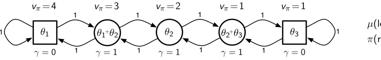
Soft termination is particularly natural in the excursion setting, where it makes it easy to define excursions of finite and definite duration. For example, consider the deterministic MDP shown in Figure 2. There are five states, three of which do not discount at all,

γ(s) = 1, and are shown as circles, and two of which cause complete soft termination,

An Emphatic Approach to Off-policy TD Learning

1 _✓2+_✓3 1 1

1

µ(left_|·) = 2/3

⇡(right_|·) = 1

✓1

1 1 1

1

1 1

✓1+✓2 ✓2 ✓3

= 1 = 1

= 1 = 0 = 0

v⇡= 1

v⇡= 1

v⇡= 2

v⇡= 3

v⇡= 4

Figure 2: A 5-state chain MDP with soft-termination states at each end.

than the return; actions are still selected in them and, dependent on the action selected, they transition to next states indefinitely without end. In this MDP there are two actions, left and right, which deterministically cause transitions to the left or right except at the edges, where there may be a self transition. The reward on all transitions is +1. The behavior policy is to select left 2/3rds of the time in all states, which causes more time to be spent in states on the left than on the right. The stationary distribution can be shown to be dµ≈(0.52,0.26,0.13,0.06,0.03)>; more than half of the time steps are spent in the

leftmost terminating state.

Consider the target policy π that selects the right action from all states. The correct value vπ(s) of each states is written above it in the figure. For both of the two rightmost

states, the right action results in a reward of 1 and an immediate termination, so their values are both 1. For the middle state, followingπ (selectingrightrepeatedly) yields two rewards of 1 prior to termination. There is no discounting (γ= 1) prior to termination, so the middle state’s value is 2, and similarly the values go up by 1 for each state to its left, as shown. These are the correct values. The approximate values depend on the parameter vector θt

as suggested by the expressions shown inside each state in the figure. These expressions use the notation θi to denote the ith component of the current parameter vector θt. In

this example, there are five states and only three parameters, so it is unlikely, and indeed impossible, to represent vπ exactly. We will return to this example later in the paper.

In addition to enabling definitive termination, as in this example, state-dependent dis-counting enables a much wider range of predictive questions to be expressed in the form of a value function (Sutton et al. 2011, Modayil, White & Sutton 2014, Sutton, Rafols & Koop 2006), including option models (Sutton, Precup & Singh 1999, Sutton 1995). For example, with state-dependent discounting one can formulate questions both about what will happen during a way of behaving and what will be true at its end. A general representation for predictions is a key step toward the goal of representing world knowledge in verifiable pre-dictive terms (Sutton 2009, 2012). The general form is also useful just because it enables us to treat uniformly many of the most important episodic and continuing special cases of interest.

A second generalization, developed for the first time in this paper, is to explicitly specify the states at which we are most interested is obtaining accurate estimates of value. Recall that in parametric function approximation there are typically many more states than pa-rameters (N n), and thus it is usually not possible for the value estimates at all states to be exactly correct. Valuing some states more accurately usually means valuing others less accurately, at least asymptotically. In the tabular case where much of the theory of reinforcement learning originated, this tradeoff is not an issue because the estimates of each state are independent of each other, but with function approximation it is necessary to

ify relative interest in order to make the problem well defined. Nevertheless, in the function approximation case little attention has been paid in the literature to specifing the relative importance of different states (an exception is Thomas 2014), though there are intimations of this in the initiation set of options (Sutton et al. 1999). In the past it was typically assumed that we were interested in valuing states in direct proportion to how often they occur, but this is not always the case. For example, in episodic problems we often care primarily about the value of the first state, or of earlier states generally (Thomas 2014). Here we allow the user to specify the relative interest in each state with a nonnegative

interest function i: S _→ [0,_∞). Formally, our objective is to minimize the Mean Square Value Error (MSVE) with states weighted both by how often they occur and by our interest in them:

MSVE(θ)=.

X

s∈S

dµ(s)i(s)

vπ(s)−θ>φ(s)

2

. (15) For example, in the 5-state example in Figure 2, we could choose i(s) = 1,_∀s _∈ S, in which case we would be primarily interested in attaining low error in the states on the left side, which are visited much more often under the behavior policy. If we want to counter this, we might chose i(s) larger for states toward the right. Of course, with parametric function approximation we presumably do not have access to the states as individuals, but certainly we could set i(s) as a function of the features in s. In this example, choosing

i(s) = 1 +φ2(s) + 2φ3(s) (where φi(s) denotes theith component ofφ(s)) would shift the

focus on accuracy to the states on the right, making it substantially more balanced. The third and final generalization that we introduce in this section is general bootstrap-ping. Conventional TD(λ) uses a bootstrapping parameter λ _∈ [0,1]; we generalize this to a bootstrapping function λ:S _→[0,1] specifying a potentially different degree of boot-strapping, 1−λ(s), for each state s. General bootstrapping of this form has been partially developed in several previous works (Sutton 1995, Sutton & Barto 1998, Maei & Sutton 2010, Sutton et al. 2014, cf. Yu 2012). As a notational shorthand, let us useλt=. λ(St) and

γt=. γ(St). Then we can define a general notion of bootstrapped return, theλ-return with

state-dependent bootstrapping and discounting:

Gλ_t =. Rt+1+γt+1

h

(1−λt+1)θ>t φt+1+λt+1Gλt+1

i

. (16) Theλ-return plays a key role in the theoretical understanding of TD methods, in particular, in their forward views (Sutton & Barto 1998, Sutton, Mahmood, Precup & van Hasselt 2014). In the forward view, Gλ_t is thought of as the target for the update at timet, even though it is not available until many steps later (when complete terminationγ(Sk) = 0 has

occurred for the first time for somek > t).

Given these generalizations, we can now specify our final new algorithm, emphatic TD(λ), by the following four equations, fort_≥0:

θt+1 =. θt+α

Rt+1+γt+1θt>φt+1−θt>φt

et (17)

et=. ρt(γtλtet−1+Mtφt), withe−1=. 0 (18)

Mt=. λti(St) + (1−λt)Ft (19)

An Emphatic Approach to Off-policy TD Learning

whereFt≥0 is a scalar memory called the followon trace. The quantityMt≥0 is termed

the emphasis on step t. Note that, if desired, Mt can be removed from the algorithm by

substituting its definition (19) into (18).

6. Off-policy Stability of Emphatic TD(λ)

As usual, to analyze the stability of the new algorithm we examine its A matrix. The stochastic update can be written:

θt+1=. θt+α

Rt+1+γt+1θt>φt+1−θ>t φt

et

=θt+α

etRt+1

| {z } bt

−et(φt−γt+1φt+1)>

| {z }

At

θt

.

Thus, A= lim

t→∞E[At] = limt→∞Eµ

h

et(φt−γt+1φt+1)>

i

=X

s

dµ(s) lim t→∞Eµ

h

et(φt−γt+1φt+1)>

St=s

i

=X

s

dµ(s) lim t→∞Eµ

h

ρt(γtλtet−1+Mtφt) (φt−γt+1φt+1)>

St=s

i

=X

s

dµ(s) lim

t→∞Eµ[(γtλtet−1+Mtφt)|St=s]Eµ

h

ρt(φt−γt+1φt+1)>

St=s

i

(because, given St,et−1 andMt are independent of ρt(φt−γt+1φt+1)>)

=X

s

dµ(s) lim

t→∞Eµ[(γtλtet−1+Mtφt)|St=s]

| {z }

e(s)∈Rn

Eµ

h

ρk(φk−γk+1φk+1)>

Sk=s

i

=X

s

e(s)Eπ[φk−γk+1φk+1|Sk=s]> (by (7))

=X

s

e(s) φ(s)−X

s0

[Pπ]ss0γ(s0)φ(s0)

!_>

=E(I₋PπΓ)Φ, (21)

whereE is anN ×n matrixE>= [. e(1),· · ·,e(N)], ande(s)∈Rn _{is defined by}5_:

e(s)=. dµ(s) lim

t→∞Eµ[γtλtet−1+Mtφt|St=s] (assuming this exists)

=dµ(s) lim

t→∞Eµ[Mt|St=s]

| {z }

m(s)

φ(s) +γ(s)λ(s)dµ(s) lim

t→∞Eµ[et−1|St=s]

=m(s)φ(s)+γ(s)λ(s)dµ(s) lim t→∞

X

¯

s,¯a

P{St−1= ¯s, At−1= ¯a|St=s}Eµ[et−1|St−1= ¯s, At−1= ¯a] 5. Note that this is a slight abuse of notation;etis a vector random variable, one per time step, and e(s)

is a vector expectation, one per state.

=m(s)φ(s) +γ(s)λ(s)dµ(s)

X

¯

s,¯a

dµ(¯s)µ(¯a|s¯)p(s|s,¯ ¯a)

dµ(s)

lim

t→∞Eµ[et−1|St−1= ¯s, At−1= ¯a]

(using the definition of a conditional probability, a.k.a. Bayes rule) =m(s)φ(s)+γ(s)λ(s)X

¯

s,¯a

dµ(¯s)µ(¯a|¯s)p(s|¯s,¯a)π(¯a|s¯)

µ(¯a_|s¯)tlim→∞Eµ[γt−1λt−1et−2+Mt−1φt−1|St−1=¯s]

=m(s)φ(s) +γ(s)λ(s)X

¯

s

X

¯

a

π(¯a_|s¯)p(s_|s,¯ ¯a)

!

e(¯s) =m(s)φ(s) +γ(s)λ(s)X

¯

s

[Pπ]ss¯ e(¯s).

We now introduce threeN_×N diagonal matrices: M, which has them(s)=. dµ(s) limt→∞

Eµ[Mt|St=s] on its diagonal;Γ, which has the γ(s) on its diagonal; andΛ, which has the

λ(s) on its diagonal. With these we can write the equation above entirely in matrix form, as

E>=Φ>M+E>PπΓΛ

=Φ>M+Φ>MPπΓΛ+Φ>M(PπΓΛ)2+· · ·

=Φ>M(I−PπΓΛ)−1.

Finally, combining this equation with (21) we obtain

A=Φ>M(I₋PπΓΛ)−1(I−PπΓ)Φ, (22)

and through similar steps one can also obtain emphatic TD(λ)’s b vector,

b=Erπ =Φ>M(I−PπΓΛ)−1rπ, (23)

whererπ is the N-vector of expected immediate rewards from each state underπ.

Emphatic TD(λ)’s key matrix, then, is M(I₋PπΓΛ)−1(I−PπΓ). To prove that it is

positive definite we will follow the same strategy as we did for emphatic TD(0). The first step will be to write the last part of the key matrix in the form of the identity matrix minus a probability matrix. To see how this can be done, consider a slightly different setting in which actions are taken according toπ, and in which 1−γ(s) and 1−λ(s) are considered probabilities of ending by terminating and by bootstrapping, respectively. That is, for any starting state, a trajectory involves a state transition according toPπ, possibly terminating