Structure Discovery in Bayesian Networks
by Sampling Partial Orders
∗Teppo Niinim¨aki [email protected]
Helsinki Institute for Information Technology Department of Computer Science
P.O. Box 68 (Gustaf H¨allstr¨ominkatu 2b) FI-00014 University of Helsinki, Finland
Pekka Parviainen [email protected]
Helsinki Institute for Information Technology Department of Computer Science
P.O. Box 15400 (Konemiehentie 2) FI-00076 Aalto, Finland
Mikko Koivisto [email protected]
Helsinki Institute for Information Technology Department of Computer Science
P.O. Box 68 (Gustaf H¨allstr¨ominkatu 2b) FI-00014 University of Helsinki, Finland
Editor:Edo Airoldi
Abstract
We present methods based on Metropolis-coupled Markov chain Monte Carlo (MC3) and
annealed importance sampling (AIS) for estimating the posterior distribution of Bayesian networks. The methods draw samples from an appropriate distribution of partial orders on the nodes, continued by sampling directed acyclic graphs (DAGs) conditionally on the sampled partial orders. We show that the computations needed for the sampling algorithms are feasible as long as the encountered partial orders have relatively few down-sets. While the algorithms assume suitable modularity properties of the priors, arbitrary priors can be handled by dividing the importance weight of each sampled DAG by the number of topological sorts it has—we give a practical dynamic programming algorithm to compute these numbers. Our empirical results demonstrate that the presented partial-order-based samplers are superior to previous Markov chain Monte Carlo methods, which sample DAGs either directly or via linear orders on the nodes. The results also suggest that the conver-gence rate of the estimators based on AIS are competitive to those of MC3. Thus AIS is the
preferred method, as it enables easier large-scale parallelization and, in addition, supplies good probabilistic lower bound guarantees for the marginal likelihood of the model.
Keywords: annealed importance sampling, directed acyclic graph, fast zeta transform, linear extension, Markov chain Monte Carlo
1. Introduction
The Bayesian paradigm to structure learning in Bayesian networks is concerned with the posterior distribution of the underlying directed acyclic graph (DAG) given data on the variables associated with the nodes of the graph (Buntine, 1991; Cooper and Herskovits, 1992; Madigan and York, 1995). The paradigm is appealing as it offers an explicit way to incorporate prior knowledge as well as full characterization of posterior uncertainty about the quantities of interest, including proper treatment of any non-identifiability issues. How-ever, a major drawback of the Bayesian paradigm is its large computational requirements. Indeed, because the number of DAGs grows very rapidly with the number of nodes, exact computation of the posterior distribution becomes impractical already when there are more than about a dozen of nodes.
There are two major approaches to handle the posterior distribution of DAGs without explicitly computing and representing the entire distribution. One is to summarize the pos-terior distribution by a relatively small number of summary statistics, of which perhaps the
most extensively used is amode of the distribution, that is, a maximum a posteriori DAG
(Cooper and Herskovits, 1992). Other useful statistics are the marginal posterior
probabil-ities of so-called structural features, such as individual arcs or larger subgraphs (Buntine,
1991; Cooper and Herskovits, 1992; Friedman and Koller, 2003). When the interest is in how well the chosen Bayesian model fits the data, say in comparison to some alternative
model, then the key quantity is the marginal likelihood of the model—also known as the
integrated likelihood, evidence, or the normalizing constant—which is simply the marginal probability (density) of the observed data. Provided that the model satisfies certain mod-ularity conditions, all these statistics can be computed in a dynamic programming fashion, and thereby avoiding exhaustive traversing through individual DAGs. Specifically,
assum-ing a very basic form of modularity one can find a mode overn-node DAGs inO(2nn2) time
(Koivisto and Sood, 2004; Ott et al., 2004; Singh and Moore, 2005; Silander and Myllym¨aki,
2006) and the arc posterior probabilities and the marginal likelihood in O(3nn) time (Tian
and He, 2009). Assuming a more convoluted form of modularity, also the latter quantities
can be computed inO(2nn2) time (Koivisto and Sood, 2004; Koivisto, 2006). In practice,
these algorithms scale up to about 25 nodes. For mode finding, there are also algorithms
based on the A∗ search heuristic (Yuan and Malone, 2013) and integer linear programming
(Bartlett and Cussens, 2013), which often can solve even larger problem instances.
The other approach is to approximate the posterior distribution by collecting a sam-ple of DAGs, each of which assigned a weight reflecting how representative the DAG is of the posterior distribution. Having such a collection at hand, various quantities, including the aforementioned statistics, can be estimated by appropriate weighted averages. Princi-pled implementations of the approach have used the Markov chain Monte Carlo (MCMC) methodology in various forms: Madigan and York (1995) simulated a Markov chain that moves in the space of DAGs by simple arc changes such that the chain’s stationary distribu-tion is the posterior distribudistribu-tion. Friedman and Koller (2003) obtained a significantly faster mixing chain by operating, not directly on DAGs, but in the much smaller and smoother
space of node orderings, or linear orderson the nodes more formally. The sampler, called
(2008) enhanced order-MCMC by presenting a sophisticated sampler based on tempering techniques, and a heuristic for removing the bias. Also other refinements to Madigan and York’s sampler have been presented (Eaton and Murphy, 2007; Grzegorczyk and Husmeier, 2008; Corander et al., 2008), however with somewhat more limited advantages over order-MCMC. More recently, Battle et al. (2010) extended Madigan and York’s sampler in yet another direction by applying annealed importance sampling (AIS) (Neal, 2001) to sam-ple fully specified Bayesian networks (i.e., DAGs equipped with the associated conditional distributions).
While the current MCMC methods for structure learning seem to work well in many cases, they also leave the following central questions open:
1. Smoother sampling spaces. Can we take the idea of Friedman and Koller (2003) fur-ther: are there sampling spaces that yield still a better tradeoff between computation time and accuracy?
2. Arbitrary structure priors. Can we efficiently remove the bias due to sampling node orderings? Specifically, is it computationally feasible to estimate posterior expecta-tions under an arbitrary structure prior, yet exploiting the smoother sampling space of node orderings? (The method of Ellis and Wong (2008) relies on heuristic arguments and becomes computationally infeasible when the data set is small.)
3. Efficient parallel computation. Can we efficiently and easily exploit parallel computa-tion, that is, to run the algorithm in parallel on thousands of processors, preferably without frequent synchronization or communication between the parallel processes. (Existing MCMC methods are designed rather for a small number of very long runs, and thus do not enable large-scale parallelization.)
4. Quality guarantees. Can we measure how accurate the algorithm’s output is? For instance, is it a lower bound, an upper bound, or an approximation to within some multiplicative or additive term? (Existing MCMC methods offer such guarantees only in the limit of running the algorithm infinitely many steps.)
In this article, we make a step toward answering these questions in the affirmative. Specifically, we advance the state of the art by presenting three new ideas, published in a preliminary form in three conference proceedings (Parviainen and Koivisto, 2010;
Ni-inim¨aki et al., 2011; Niinim¨aki and Koivisto, 2013b), and their combination that has not
been investigated prior to the present work. The next paragraphs give an overview of our contributions.
We address the first question by introducing a sampling space, in which each state is a partial order on the nodes. Compared to the space of node orderings (i.e., linear orders on the nodes), the resulting sampling space is smaller and the induced sampling distribution is smoother. We will also show that going from linear orders to partial orders does not increase the computational cost per sampled order, as long as the partial orders are sufficiently thin, that is, they have relatively few so-called downsets. These algorithmic results build on
and extend our earlier work on finding an optimal DAG subject to a given partial order
To address the second question, we take a somewhat straightforward approach: per sampled partial order, we draw one or several DAGs independently from the corresponding conditional distribution, and assign each DAG a weight that compensates the difference of the structure prior of interest and the “proxy prior” we employ to make order-based sampling efficient. Specifically, we show that the number of linear extensions (or, topological sorts) of a given DAG—that we need for the weight—can be computed sufficiently fast in practice for moderate-size DAGs, even though the problem is #P-hard in general (Brightwell and Winkler, 1991).
Our third contribution applies both to the third and the fourth question. Motivated by the desire for accuracy guarantees, we seek a sampler such that we know exactly from which distribution the samples are drawn. Here, the annealed importance sampling (AIS) method of Neal (2001) provides an appealing solution. It enables drawing independent and identically distributed samples and computing the associated importance weights, so that the expected value of each weighted sample matches the quantity of interest. Due to the independence of the samples, already a small number of samples may suffice, not only for producing an accurate estimate, but also for finding a relatively tight, high-confidence lower bound on the true value (Gomes et al., 2007; Gogate et al., 2007; Gogate and Dechter, 2011). Furthermore, the independence of the samples renders the approach embarrassingly parallel, requiring interaction of the parallel computations only at the very end when the independent samples are collected in a Monte Carlo estimator. We note that Battle et al. (2010) adopted AIS for quite different reasons. Namely, due to the structure of their model, they had to sample fully specified Bayesian networks whose posterior distribution is expected to be severely multimodal, in which case AIS is a good alternative to the usual MCMC methods. Finally, we evaluate the significance of the aforementioned advances empirically. As a benchmark we use Friedman and Koller’s (2003) simple Markov chain on the space of node orderings, however, equipped with the Metropolis-coupling technique (Geyer, 1991)
to enhance the chain’s mixing properties. Our implementation of the Metropolis-coupled
MCMC (MC3) method for the space of node orderings also serves as a proxy of a related
implementation1 of Ellis and Wong (2008). Our experimental study aims to answer two
main questions: First, does the squeezing of the space of linear orders into a space of partial orders yield a significantly faster mixing Markov chain when we already use the Metropolis coupling technique to help mixing? This question was left unanswered in our preliminary
work (Niinim¨aki et al., 2011) that only considered a single simple Markov chain similar
to that of Friedman and Koller (2003). Second, are the Monte Carlo estimators based on
AIS competitive to the MC3-based estimators when we sample partial orders instead of
linear orders? This question was left unanswered in our preliminary work (Niinim¨aki and
Koivisto, 2013b) that only considered sampling linear orders.
The remainder of this article is organized as follows. We begin in Section 2 with an introduction to some basic properties of graphs and partial orders. The section also contains some more advanced algorithmic results, which will serve as building blocks of our method for learning Bayesian networks. In Section 3, we review the Bayesian formulation of the structure learning problem in Bayesian networks, and also outline the approach of Friedman and Koller (2003) based on sampling node orderings. In Section 4, we extend the idea of
sampling node orderings to partial orders and formulate the two sampling methods, MC3 and AIS, in that context. We dedicate Section 5 to the description of fast algorithms for computing several quantities needed by the samplers. Experimental results are reported in Section 6. We conclude and discuss directions for future research in Section 7.
2. Partial Orders and DAGs
This section introduces concepts, notation, and algorithms associated with graphs and partial orders. In later sections, we will apply them as building blocks in the context of structure learning in Bayesian networks. The content of the first subsection will be needed already in Section 3. The content of the latter subsections will be needed only in Section 5, and the reader may wish to skip them on the first read.
2.1 Antisymmetric Binary Relations
We use the standard concepts of graphs and partial orders. Our notation is however
some-what nonstandard, which warrants a special attention. Let N be a finite set, and let
R ⊆N ×N be a binary relation on N. We shall denote an element (u, v) of R by uv for
short. We say thatR is
reflexive ifu∈N implies uu∈R; antisymmetric ifuv, vu∈R impliesu=v;
transitive ifuv, vw∈R implies uw∈R;
total ifu, v∈N implies uv∈R orvu∈R .
IfRhas the first three properties, it is called apartial order. If it has all the four properties,
it is called a total or linear order. The set N is the ground set of the order and the pair
(N, R) is called a linearly or partially ordered set.
We will also consider relations that are antisymmetric but that need not have any other
of the above the properties. We say that R is
acyclic if there are no elements u1, . . . , ul such that
u1 =ul and ui−1ui∈R for each i= 2, . . . , l .
Note that acyclicity implies irreflexivity, that is, that uu6∈R for all u∈N. IfR is acyclic,
we call the pair (N, R) a directed acyclic graph(DAG),N itsnode set, and R its arc set.
When the set N is clear from the context—as it will often be in our applications—we
identify the structure (N, R) with the relation R. We will typically use the letters P, L,
and A for a partial order, linear order, and a DAG, respectively.
The following relationships among the three objects are central in later sections of this
article. Let R and Q be relations on N. We say that Q is an extension of R if simply
R ⊆ Q. If Q is a linear order, then we may also call it a linear extension of R. Note
that in the literature, a linear extension of a DAG is sometimes called a topological sort of
the DAG. Sometimes we will be interested in the number of linear extensions of R, which
we denote by `(R). Furthermore, we say that R and Q are compatible with each other if
they have a common linear extension L ⊇ R, Q. While this relationship is symmetric, in
1 3
2
4
6 5
8 7
1 3
2
4
6 5
8 7
Figure 1: The Hasse diagram of a partial order on eight nodes (left) and a DAG compatible with the partial order (right).
1
3 2
3 1 2
1
3 2
3 1 2
3 2 1
2 3 1
A1 A2 A3 L1 L2 L3
1 2 3
L4
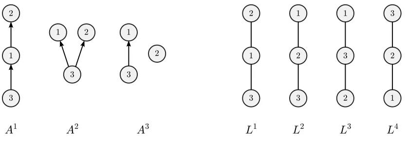
Figure 2: Three DAGs (left) and the Hasse diagrams of four linear orders (right), some
of which are compatible with some of the DAGs. DAG A1 has only one linear
extension: L1. DAGA2 has two linear extensions: L1 andL2. DAGA3 has three
linear extensions: L1,L2 and L3. None of the DAGs is compatible with L4.
we say that Q is the transitive closure of R if Q is the minimal transitive relation that
contains R. Finally, we say that R is the transitive reduction of Q if R is the minimal
relation with the same transitive closure asQ. The transitive reduction of a partial orderQ
is sometimes called the covering relationand visualized graphically by means of the Hasse
diagram. Figures 1 and 2 illustrate some of these concepts.
Some of the above described relationships can be characterized locally, in terms of the
in-neighbors of each element of N. To this end we let Rv denote the set of elements that
precedev inR, formally
Rv ={u:uv∈R, u6=v}.
We will call the elements ofRv theparents of v and the set Rv theparent set of v. If R is
a partial order we may call the parents also the predecessors of v. We observe that ifQ is
;
f6g f1g f5g f1,6g f5,6g f1,5g f5,8g f1,5,6g f4,5,6g f5,6,8g f1,5,8g
f1,2,3,4,5,6,7,8g
f1,3,4,5,6,7,8g f1,2,3,4,5,6,8g
f1,2,3,4,5,6,7g
f1,2,3,4,5,6g f1,3,4,5,6,7g f1,3,4,5,6,8g
f1,3,4,5,6g f1,3,5,6,8g f1,4,5,6,8g
f1,3,5,6g f1,4,5,6g f1,5,6,8g f1,4,5,8g
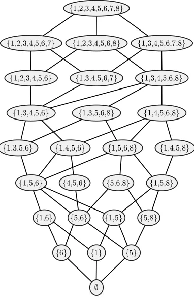
Figure 3: The covering graph of the downset lattice of the partial order shown in Figure 1.
2.2 Downsets and Counting Linear Extensions
LetP be a partial order on a setN. A subsetY ⊆N is adownset ofP ifv∈Y anduv ∈P
imply thatu∈Y. In the literature downsets are sometimes called also order ideals or just
ideals. We denote the set of downsets by D(P), or shorter D when there is no ambiguity
about the partial order. Thedownset latticeofP is the set of downsets ordered by inclusion,
(D,⊆). While we do not define the notion of lattice here, we note that every lattice is a
partially ordered set and thus can be represented by itscovering graph, that is,Dequipped
with the covering relation. An example of a covering graph is shown in Figure 3. Observe
that in the covering graph a node X is a parent of another node Y if and only if X is
obtained from Y by removing some maximal element ofY, that is, an element of
maxY =u∈Y :uv 6∈P for all v∈Y \ {u} .
(Later we may use the notation maxY also for a setY that is not a downset.)
The following result of Habib et al. (2001) guarantees us an efficient access to the downset lattice of a given partial order:
Remark 2 Actually Habib et al. (2001) show a stronger result, namely that the factor n in the time and space complexity can be reduced to the width of the partial order.
As a first use of these concepts we consider the problem of counting the linear extensions
of a given partial orderP on N. Recall that we denote this count by`(P). It is immediate
that `(P) equals the number of paths from the empty set ∅ to the ground set N in the
covering graph of the downset lattice of P. Thus, letting F(∅) = 1 and, recursively for
nonemptyY ∈ D,
F(Y) = X
v∈Y Y\{v}∈D
F Y \ {v} ,
we have thatF(N) =`(P). This result is a special case of Lemma 18 that will be given in
Section 5.2. Because the covering graph provides us with an efficient access to the downsets and their parents in the covering graph, we have the following result:
Theorem 3 Given a partial orderP on ann-element set, the number of linear extensions of P can be computed in O(n|D|) time and space.
This result extends to counting the linear extensions of a given DAG A. Namely, we
observe that`(A) equals the number of linear extensions of the partial order P(A) that is
obtained by taking the transitive closure of A and adding the self-loop vv for each node
v ∈ N. The transitive closure can be computed relatively fast, in O(n3) time, using the
Floyd–Warshall algorithm.
Corollary 4 Given a DAG A on an n-element set, the number of linear extensions of A can be computed in O n3+n|D(P(A))|
time and O n|D(P(A))| space.
Remark 5 In the worst case the number of downsets is 2n. We are not aware of any
algorithm that would compute the exact number of linear extensions faster than inO(n2n)
time in the worst case. As the problem is #P-complete (Brightwell and Winkler, 1991), there presumably is no polynomial time exact algorithm for the problem. It is possible to approximate the count to within any relative error ε >0, roughly, in O(ε−2n5log3n) time (see Sect. 4 of Bubley and Dyer, 1999). Unfortunately, the large hidden constants and the large degree of the polynomial render the approximation algorithms impractical even for
moderate values of ε. It is also known that the linear extensions of P can be enumerated
in constant amortized time, which enables counting in O(n2 +`(P)) time (Pruesse and
Ruskey, 1994; Ono and Nakano, 2005). However, the enumeration approach to counting is
not feasible when `(P) is large.
2.3 Fast Zeta Transforms
Denote by 2N the power set of N and by
R the set of real numbers. For a function
ϕ: 2N →Rthezeta transformofϕover the subset lattice (2N,⊆) is the functionϕb: 2
N →
R defined by
b
ϕ(Y) = X X⊆Y
We shall introduce two computational problems that concern the evaluation of the zeta transform in restricted settings where the input function is sparse (has a small support) and
also the output function is evaluated only at some subsets. In theinflating zeta transform
problem we are given a partial orderP onN, a functionϕ:D →Rfrom the downsets ofP
to real numbers, and an arbitrary collection C of subsets ofN. The task is to compute the
zeta transform ϕb restricted to C, that is, to compute ϕb(Y) for every Y ∈ C. To make the
formula (1) applicable, we understand thatϕ(X) = 0 forX ∈2N\ D. In thedeflating zeta
transform problem we are given a partial orderP on N, a collectionCof subsets ofN, and
a functionϕ:C →R. The task is to compute the zeta transform ϕbrestricted toD. Again,
we understand that ϕ(X) = 0 for X ∈ 2N \ C. Clearly, the problems coincide if we take
C=D, and the resulting transform is known as the zeta transform over the downset lattice.
In these problems we assume that the input function is given as a list of argument–value
pairs (X, ϕ(X)), whereX ranges over the domain of the function (i.e., C orD).
We begin with the problem of computing a zeta transform over the downset lattice:
Theorem 6 Given a partial order P on an n-element set and a function ϕ:D →R, the zeta transform of ϕ over the downset lattice (D,⊆) can be computed in O(n|D|) time and space.
To prove this result we consider the following algorithm. First construct the covering
graph of the downset lattice and associate each downset Y with the value ϕ0(Y) = ϕ(Y).
Then find an ordering v1, . . . , vn of the elements of N such that vivj ∈ P implies i ≤ j.
Next, for each downset Y and for each i= 1, . . . , n, let
ϕi(Y) =ϕi−1(Y) +
ϕi−1(Y \ {vi}) ifvi∈Y and Y \ {vi} ∈ D,
0 otherwise.
Finally return the values ϕn(Y) for Y ∈ D. We can show that the algorithm is correct:
Lemma 7 It holds that ϕn(Y) =ϕb(Y) for all Y ∈ D.
The proof of this lemma and Lemmas 9–11 below are given in the appendix.
To complete the proof of Theorem 6, it remains to analyze the time and space require-ments of the algorithm. The time and space requirement of constructing the covering graph
are within the budget by Theorem 1. Finding a valid ordering takes O(n2) time and space
using standard algorithms for topological sorting. Finally, for each Y ∈ D, running the n
steps and storing the valuesϕi(Y) takes O(n) time and space, thus O(n|D|) in total. Note
that the covering graph representation enables constant-time accessing of the downsets
Y \ {vi}for a given downset Y.
Let us then turn to the two more general problems.
Theorem 8 The deflating zeta transform problem and the inflating zeta transform problem can be solved in O(n2|C|+n|D|) time and O(n|C|+n|D|) space.
We prove first the claim for the deflating zeta transform problem. We develop our algorithm in two stages so as to split the sum in the zeta transform into two nested sums:
the outer sum will be only over the downsets X of P, while the inner sum will gather the
The key concept is the tail of a downsetY, which we define as the set interval
TY ={X: maxY ⊆X⊆Y}.
The following lemma shows that the tails are pairwise disjoint.
Lemma 9 Let Y andY0 be distinct downsets. Then the tailsTY and TY0 are disjoint.
We also have that each subset of the ground set belongs to some tail:
Lemma 10 Let X ⊆ N. Let Y ={u :uv ∈ P, v ∈ X}, that is, the downward-closure of X. Then Y ∈ D and X∈ TY.
Lemmas 9 and 10 imply that for any downset S ∈ D the tails
TY : Y ∈ D ∩2S
partition the power set 2S. This allows us to split the zeta transform into two nested
summations. Let
β(Y) = X X∈TY
ϕ(X), forY ∈ D.
Now
b
ϕ(Y) =βb(Y) = X
X⊆Y X∈D
β(X), forY ∈ D.
Our algorithm computesϕbin two stages: first, givenϕ, it evaluatesβ at all downsets of P;
second, givenβ, it evaluates ϕbat all downsets ofP. We have already seen how the second
stage can be computed within the claimed time and space budget (Theorem 6).
The first stage is computationally relatively straightforward, since each X ∈ C
con-tributes to exactly one term β(Y). Specifically, we can compute the function β by
initial-izing the values β(Y) to zero, then considering each X ∈ C in turn and incrementing the
value β(Y) by ϕ(X) for the unique downset Y satisfying X ∈ TY. Using the observation
that Y is the downward-closure of X, as given by Lemma 10, the set Y can be found in
O(n2) time. This completes the proof of the first claim of Theorem 8.
Consider then the inflating zeta transform problem. We use the same idea as above, however, reversing the order of the two stages. Specifically, the algorithm first computes
the zeta transform over the downset lattice D, resulting in the values ϕb(Y) for all Y ∈ D.
Then, the algorithm extends the output function to the domain C using the observation
that the zeta transform is piecewise constant, that is, for anyZ ⊆N we haveϕb(Z) =ϕb(Y)
for a unique downsetY:
Lemma 11 Let Z ⊆N. Then D ∩2Z=D ∩2Y, where the set Y ∈ D is given by
Y ={v∈Z :if uv ∈P, then u∈Z};
in words, Y consists of all elements of Z whose predecessors also are in Z.
Clearly the set Y can be constructed in O(n2) time for a given set Z. This completes the
Remark 12 The zeta transforms studied in this subsection have natural “upward-variants”
where the condition X ⊆ Y is replaced by the condition X ⊇ Y. The presented results
readily apply to these variants, by complementation. Indeed, letting P be a partial order
on N and denoting by ¯Y the complement N \ Y and by ¯P the reversed partial order
{vu:uv∈P}, we have the equivalences
X ⊇Y ⇐⇒ X¯ ⊆Y¯ and Y ∈ D(P) ⇐⇒ Y¯ ∈ D( ¯P).
Thus an upward-variant can be solved by first complementing the arguments of the in-put function, then solving the “downward-variants”, and finally complementing back the arguments of the output function.
2.4 Random Sampling Variants
The above described zeta transform algorithms compute recursively large sums of
nonneg-ative weights ϕ(Z) each corresponding to a subsetZ ⊆N. Later we will also need a way
to draw independent samples of the subsets Z ⊆ Y, proportionally to the weights.
Coin-cidentally, the introduced summation algorithms readily provide us an efficient way to do this: for each sample we only need to stochastically backtrack the recursive steps.
We illustrate this generic approach to extend a summation algorithm into a sampling algorithm by considering the deflating zeta transform problem. Suppose we are given a
partial order P on N, a collection of C of subsets of N, and a function ϕ : C 7→ R. As
an additional input we now also assume a downset Y ∈ D. We consider the problem of
generating a random subset Z ∈ C ∩2Y proportionally to ϕ(Z). We show next that this
problem can be solved in O(n) time, provided that the deflating zeta transform has been
precomputed and the intermediate results are stored in memory.
In the first stage the algorithm backtracks the zeta transform over the downset lattice,
as follows. Let Yn=Y. For i=n, n−1, . . . ,1,
ifYi\ {vi} ∈ D, then with probabilityβi−1(Yi\ {vi})
βi(Yi) letYi−1 =Yi\ {vi};
otherwise letYi−1 =Yi.
By the proof of Theorem 6, the resulting setY1is a random draw from the subsets inD ∩2Y
proportionally toβ(Y1). This first stage takes clearly O(n) time.
In the second stage the algorithm generates a random set X ∈ TY1 proportionally to
ϕ(X). In this case, the number of alternative options is not constant, and we need an
efficient way to sample from the respective discrete probability distribution. A particularly
efficient solution to this subproblem is known as the Alias method (Walker, 1977; Vose,
1991):
Theorem 13 (Alias method) Given positive numbersq1, q2, . . . , qr, one can inO(r)time construct a data structure, which enables drawing a random i∈ {1, . . . , r} proportionally to qi in constant time.
We can view the list of the terms ϕ(X), for X ∈ TY1, as an intermediate result, which
has been precomputed and stored in memory using the Alias method. Thus the second
3. Bayesian Learning of Bayesian Networks
In this section we review the Bayesian approach to structure learning in Bayesian networks. Our emphasis will be on the notion of modularity of the various components of the Bayesian model. From the works of Friedman and Koller (2003) and Koivisto and Sood (2004) we also adopt the notion of order-modularity that is central in the partial-order-MCMC method, which we introduce in the next section.
3.1 The Bayesian Approach to Structure Learning
We shall consider probabilistic models forn attributes, thevth attribute taking values in a
set Xv. We will also assume the availability of a data set D consisting of m records over
the attributes. We denote byDjv the datum for thevth attribute in thejth record. We will
denote byN the index set{1, . . . , n}, and often apply indexing by subsets. For example, if
S ⊆N, we writeDSj for{Djv :v∈S} and simplyDj forDjN.
We build a Bayesian network model for the data a priori, before seeing the actual data.
To this end, we treat each datum Dvj as a random variable with the state space Xv. We
model the random vectors Dj = (Dj1, . . . , Djn) as independent draws from an n-variate
distribution θ which is Markov with respect to some directed acyclic graph G = (N, A),
that is,
θ(Dj) = Y v∈N
θ(Dvj|DjA
v). (2)
Recall thatAv ={u:uv∈A}denotes the set of parents of node v inG. We call the pair
(G, θ) a Bayesian network, G its structure, and θ its parameter. As our interest will be
in settings where the node set N is considered fixed, whereas the arc set A varies, we will
identify the structure with the arc setA and dropGfrom the notation.
Because our interest is in learning the structure from the data, we include the Bayesian
network in the model as a random variable. Thus we compose a joint distributionp(A, θ, D)
as the product of a structure prior p(A), a parameter prior p(θ |A), and the likelihood
p(D|A, θ) =Q
jθ(Dj). Once the dataDhave been observed, our interest is in thestructure
posterior p(A|D), which, using Bayes’s rule, is obtained as the ratio p(A)p(D|A)/p(D),
wherep(D|A) is thestructure likelihoodandp(D) themarginal likelihood. Note that as the
parameter θ is not of direct interest, it is marginalized out. With suitable choices of the
parameter prior, the marginalization can be carried out analytically; we will illustrate this below in Example 1.
Various quantities that are central in structure discovery, as well as in prediction of yet unobserved data, can be cast as the posterior expectation
E(f|D) =
X
A
f(A)p(A|D) (3)
of some functionf that associates each structureAwith a real number, or more generally, an
element of a vector space. For example, if we letf be the indicator function of the structures
where s is a parent of t, then E(f|D) equals the posterior probability that st ∈ A. For
another example, define f in relation to the observed data D and to unobserved data D0
distributionp(D0|D). Note that in this instantiation we allowed the functionf depend on
the observed data D, which is only implicitly enabled in the expression (3). The marginal
likelihood p(D) is yet another variant of (3), obtained as theprior expectation E(f) of the
functionf(A) =p(D|A). We will generally refer to the functionf of interest as thefeature.
3.2 Modularity and Node Orderings
From a computational point of view, the main challenge is to carry out the summation
over all possible structures A, either exactly or approximately. As the number of possible
structures grows very rapidly in the number of nodes, the hope is in exploiting the properties of both the posterior distribution and the feature. Here, a central role is played by functions that are modular in the sense that they factorize into a product of “local” factors, one term
per pair (v, Av), in concordance with the factorization (2).
We define the notion of modularity so that it applies equally to features, structure prior,
and structure likelihood. Let ϕbe a mapping that associates each binary relation R on N
with a real number. We say thatϕismodularif for each nodev there exists a mappingϕv
from the subsets of N \ {v} to real numbers such thatϕ(R) =Q
v∈Nϕv(Rv). We call the
functions ϕv thefactors of ϕ.
In what follows, the relation R will typically be the arc set of a DAG. For example,
the indicator function for a fixed arc st mentioned above is modular, with the factors fv
satisfying fv(Av) = 0 if v=t and s6∈Atand fv(Av) = 1 otherwise.
Modular structure priors can take various specific forms. For example, a simple prior is
obtained by assigning each node pair uv a real number κuv>0 and letting the prior p(A)
be proportional to κ(A) = Q
uv∈Aκuv. Such prior allows giving separate weight for each
arc according to its prior plausibility. The uniform prior is a special case where κuv = 1
for all node pairs uv. Note that proportionality guarantees modularity, since the nfactors
of the prior can absorb the normalizing constant c = P
Aκ(A), for example, by setting
thevth factor toκv(Av)c−1/n. Another example is the prior proposed by Heckerman et al.
(1995), that penalizes the distance betweenAand a user-defined prior DAGA0. This can be
obtained by lettingp(A) be proportional toQ
v∈Nκv(Av) whereκv(Av) =δ|(Av∪A
0
v)\(Av∩A0v)|
and 0< δ≤1 is a user-defined constant that determines the penalization strength. Modular
structure priors also enable a straightforward way to bound the indegrees of the nodes.
Indeed, we often consider the case where p(A) vanishes if there exists a node v for which
|Av| exceeds some fixed maximum indegree, denoted by k. Note, however, that modular
structure priors do not allow similar controlling of the outdegrees of the nodes. For a node
vwe will call a setS apotential parent set if the prior does not vanish whenS is the parent
set of v, that is, p(A) >0 for some structureA with Av =S. Specifically, if p is modular,
thenS is a potential parent set ofv if and only if pv(S)>0.
The following example describes a frequently used modular structure likelihood (Bun-tine, 1991; Heckerman et al., 1995):
Example 1 (Dirichlet–multinomial likelihood) Suppose that each setXvis finite.
Con-sider a fixed structureA⊆N×N. For each nodevand its parent setAv, let the conditional
distribution of Dvj given DjAv = y be categorical with parameters θv·y ={θvxy : x ∈ Xv}.
Define a distribution θ of Dj as the product of the conditional distributions and observe
parameters rvxy >0, for x∈ Xv, and compose the priorp(θ|A) by assuming independence
of the components. Let mvxy denote the number of data records j where Dvj = x and
DjAv =y. Then
p(D|A) =
Z
p(θ|A)p(D|A, θ)dθ
= Y
v∈N Y
y∈XAv
Γ(rv·y)
Γ(rv·y+mv·y)
Y
x∈Xv
Γ(rvxy+mvxy)
Γ(rvxy) ,
whererv·y and mv·y are the sums of the numbers rvxy and mvxy, respectively, and Γ is the
gamma function. In an important special case, each parameter rvxy is set to a so-called
equivalent sample size α≥0 divided by the number of joint configurations ofx andy (i.e.,
by |Xv|ifAv is empty and by|Xv||XAv|otherwise).
By a modular model we will refer to a Bayesian model, where both the structure likeli-hood and the structure prior are modular. We will assume that such a model is represented
in terms of the factorsλv andκv of a likelihoodλand an unnormalized priorκ, respectively.
In our empirical study we have used the following simple model:
Example 2 (uniform Dirichlet–multinomial model, UDM) In this modular model,
the structure prior is specified by letting κv(Av) = 1 if |Av| ≤ k, and κv(Av) = 0
other-wise. The likelihood is the Dirichlet–multinomial likelihood with the equivalent sample size
parameter set to 1 (see Example 1). The maximum indegreekis a parameter of the model.
For a demonstration of the computational benefit of modularity, let us consider the
probability (density) of the data Dconditioning on the constraint that the unknown DAG
Ais compatible with a given linear orderLon the nodes. We may express this compatibility
constraint by writing simplyL, and hence the quantity of interest byp(D|L). Write first
p(D|L) = X A
p(A, D|L) =
P
A⊆Lp(A)p(D|A) P
A⊆Lp(A)
=
P
A⊆Lκ(A)λ(A) P
A⊆Lκ(A) .
Here the last equality holds because the normalizing constants of the prior cancel out.
Then we use the key implication of the constraint A ⊆L, namely, that the set of possible
structures A decomposes into a Cartesian product of the sets of potential parent sets Av
for each nodev (Buntine, 1991; Cooper and Herskovits, 1992):
p(D|L) = Y v∈N
X
Av⊆Lv
κv(Av)λv(Av) ,
Y
v∈N X
Av⊆Lv
κv(Av). (4)
This factorization enables independent processing of the parent sets for each node, which amounts to significant computational savings compared to exhaustive enumeration of all possible structures. A similar factorization can be derived for the conditional posterior
expectationE(f|D, L) of a modular featuref.
Motivated by the savings, Friedman and Koller (2003) addressed the unconstrained
of linear orders drawn from a distribution that is proportional to the marginal likelihood
p(D|L), as we will describe in the next subsection. For exact averaging over all linear
orders, Koivisto and Sood (2004) gave exponential-time dynamic programming algorithm. We will obtain that algorithm as a special case of the algorithm we give in Section 5.
When the modularity is exploited as described above, the actual joint model of the data and structures does not remain modular. This is essentially because some DAGs are consistent with fewer linear orders than other DAGs. We will discuss this issue further at the end of the next subsection. To characterize the model, for which the node-ordering
based methods work correctly, we follow Koivisto and Sood (2004) and call a model
order-modular if the likelihood function is modular and the structure prior p(A) is proportional
to κ(A)P
L⊇Aµ(L), for some modular functions κ and µ. Thus an order-modular model
can be interpreted as a “modular” joint model for the structure A and the linear orderL.
Note, that ifµ(L)>0 for all linear orders L, then the support of such a prior contains the
same DAGs as the support of the corresponding modular prior determined by κ. We will
also use the terms order-modular priorand order-modular posterior in an obvious manner.
Example 3 (order-modular UDM) In this model, the structure likelihood and the
fac-tors κv are as in a modular UDM (see Example 2), and the maximum indegree k is a
parameter of the model. The difference to the modular UDM is that we specify instead an
order-modular prior by lettingµ(L) = 1 for all linear ordersL on N. Thus the prior p(A)
is proportional to κ(A)`(A).
3.3 Sampling-based Approximations
We next review the basic sampling-based approaches for structure learning in Bayesian networks. For a broader introduction to the subject in the machine learning context, we refer to the survey by Andrieu et al. (2003).
Importance sampling methods provide us with a generic approach to approximate the
expectationE(f|D) by a sample average
1 T
T X
t=1
f(At)p(At|D)
q(At) , A
1, A2, . . . , AT ∼q(A), (5)
where q(A) is some appropriate sampling distribution. It would be desirable that (i)q(A)
is as close to the function|f(At)p(At|D)|as possible, up to a multiplicative constant, and
(ii) that the samplesAtare independent. In order to compute the average we also need, for
any given sampleAt, (iii) an access to the valueq(At) either exactly or up to a small error.
If the function q can be evaluated only up to a constant factor, then one typically uses
theself-normalized importance sampling estimate, which is obtained by dividing the sample
average (5) by the sample average of 1/q(At). In practice, it is possible to simultaneously
satisfy only some of the desiderata (i–iii).
The structure-MCMC method of Madigan and York (1995), in particular, draws the
samples by simulating a Markov chain whose stationary distribution isp(A|D). Thus, while
the sampling distribution tends top(A|D) in the limit, after a finitely many simulation steps
could be obtained with a smaller number of independent samples. Finally, the computation
ofq(At) is avoided by assuming it to be a good approximation top(At|D) and thus canceling
in the estimator. The performance of structure-MCMC depends crucially on the mixing rate of the Markov chain, that is, how fast the chain “forgets” its initial state so that the
draws will be (approximately) fromp(A|D). The main shortcoming of structure-MCMC is
that the chain may get easily trapped at small regions near local maxima of the posterior. The order-MCMCmethod of Friedman and Koller (2003), which we already mentioned in the previous subsection, aims at better performance by sampling node orderings from
a distribution that is proportional to p(D | L). Compared to the space of DAGs, the
space of node orderings is not only significantly smaller but it also smoothens the sampling
distribution, because for anyLthe marginal likelihoodp(D|L) is a sum over exponentially
many DAGs. The resulting estimator becomes
1 T
T X
t=1
E(f|D, Lt), L1, L2, . . . , LT ∼p0(L|D),
wherep0(L|D)∝p(D|L)p0(L) is obtained viap(D|L) by re-modelling then! possible node
ordering constraints L as mutually exclusive events, assigned with a uniform prior, p0(L).
In cases where exact computation of the expectation E(f|D, Lt) is not feasible, it can, in
turn, be approximated by a single evaluation at a sampled DAG,
f(At), At∼p(A|D, Lt),
or, more accurately, by an average over several independent samples from p(A|D, Lt).
Importantly, the latter sampling step, if needed, is again computationally easy thanks to the fixed node ordering. Thus the difficulty of sampling only concerns the sampling of node orderings. Friedman and Koller (2003) showed that simple local changes, namely swaps of two nodes, yield a Markov chain that mixes relatively fast in their sets of experiments. We omit a more detailed description of the order-MCMC method here, as the method is obtained as a special instantiation of the method we will introduce in Section 4.
The innocent-looking treatment of node ordering constraints as mutually exclusive events, however, introduces a “bias” to the estimator. Indeed, it is easy to see that the
samplesAt will be generated from the distribution
X
L⊇A
p0(L|D)p(A|D, L)∝p(A|D)`(A).
In other words, compared to sampling from the true posterior p(A|D), sampling via node
orderings favors DAGs that are compatible with larger numbers of linear orders. But also a different interpretation is valid: the DAGs are sampled from the correct posterior under a
modified (order-modular) model where the original, modular structure priorp(A) is replaced
by the order-modular prior that is proportional top(A)`(A) (as in Example 3). Oftentimes,
4. Sampling Partial Orders
Our key idea is to extend the order-MCMC of Friedman and Koller (2003) by replacing the state space of node orderings by an appropriately defined space of partial orders on the nodes. Throughout this section we will denote (perhaps counter to the reader’s anticipation)
by π0 the modular posterior distribution and by π its “biased” order-modular counterpart
that arises due to treating node orderings as mutually exclusive events. Our goal is to
perform Bayesian inference under the modular posterior π0. Because our approach is to
sample from the order-modular posterior π, we obtain, as a by-product, also an inference
method for order-modular models. When needed, we will refer to the underlying modular
model byp0 and to the induced order-modular model byp.
4.1 Sampling Spaces of Partial Orders
We will consider sampling from a state space that consists of partial orders on the node set
N. We will denote the state space byP. The idea is that the states inP partition the set
of all linear orders onN. To this end, we requireP to be anexact coveronN, that is, every
linear order on N must be an extension of exactly one partial order P in P. Examples 4
and 5 below illustrate the concept and also introduce the notion of a bucket order, which is central in our implementation of the proposed methods.
Example 4 (bucket orders) A partial orderB is abucket order if the ground set admits
a partition into pairwise disjoint sets,B1, B2, . . . , Bh, called thebuckets, such thatuv∈Bif
and only ifu=v oru∈Bi and v∈Bj for some i < j. Intuitively, the order of elements in
different buckets is determined by the buckets’ order, while within each bucket the elements
are incomparable. We say that the bucket order is oftype(b1, b2, . . . , bh), whenbi is the size
of Bi. We call the bucket order a balanced bucket order with a maximum bucket size b if
b=b1 =b2 =· · ·=bh−1 ≥bh. Furthermore, we call two bucket orders reorderings of each
other if they have the same ground set and they are of the same type. It is immediate that
the set (equivalence class) of reorderings of a bucket order P constitute an exact cover on
their common ground set (Koivisto and Parviainen, 2010). For a later reference, we also
note that the number of downsets of the bucket order is 1 +P
i(2bi−1). The next example gives a straightforward extension of bucket orders.
Example 5 (parallel bucket orders) A partial orderPis a parallel composition of bucket
orders, or parallel bucket order for short, if P can be partitioned into r bucket orders
B1, B2, . . . , Bron disjoint ground sets. We call two parallel bucket ordersP and Q
reorder-ingsof each other if their bucket orders can be labelled asP1, P2, . . . , PrandQ1, Q2, . . . , Qr
such that each Pj is a reordering of Qj. It is known that the set (equivalence class) of
re-orderings of a parallel bucket orderP is an exact cover on their common ground set (Koivisto
and Parviainen, 2010). Compared to bucket orders, parallel bucket orders make it possible to obtain better time–space tradeoffs in the context of exact structure discovery. However,
our preliminary calculations (Niinim¨aki et al., 2011) show that parallel bucket orders are
unlikely to yield substantive advantages in the sampling context.
swap(2,4) 1
3
2 4
1 2
3 4
1 2
4 3
2 1
3 4
2 1
4 3
3 1
4 2
swap(1,2) swap(1,2)
swap(2,3)
swap(2,4)
swap(2,3) swap(1,3)
swap(1,3) swap(1,4)
swap(1,4) swap(3,4) swap(3,4)
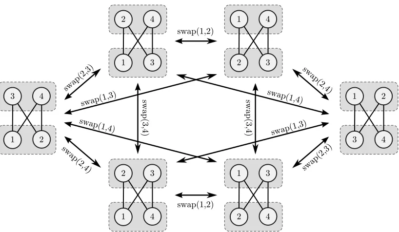
Figure 4: All reorderings of a bucket order of type (2,2) on the node set {1,2,3,4}.
Ad-jacency in the swap neighborhood is indicated by arrows labeled by the corre-sponding swap operation. Each bucket order is visualized using a Hasse diagram, with rectangles indicating individual buckets.
1 3
2
4
6 5
8 7
1 3
5
4
6 2
8 7
swap(2,5) swap(3,1)
3 1
5
4
6 2
8 7
Figure 5: Three adjacent states in the space of reorderings of a bucket order of type (3,3,2).
structure on P is just a graph on P, the adjacency relation specifying the neighborhood
relation. Here, we do not make an attempt to give any specific neighborhood structure that
would be appropriate for an arbitrary exact coverP. Instead, we continue with an example:
Example 6 (swap neighborhood) Let P be a (parallel) bucket order on N, and letP
the set of reorderings of P. Theswap neighborhood onP is a graph in which the vertex set
2 1
3
3 2 1
2 3 1
=
+
1 2
3
3 1 2
1 3 2
=
+
1 3
2
2 1 3
1 2 3
=
+
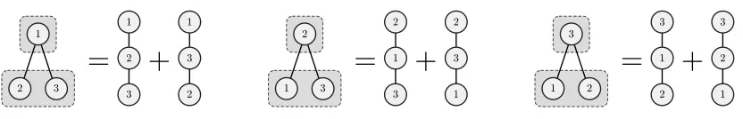
Figure 6: There are in total six linear orders on the node set{1,2,3}and three reorderings
of a bucket order of type (2,1). As shown in the figure, the probability of each bucket order is the sums of the probabilities of its linear extensions. Observe, how the bucket orders form an exact cover and hence partition the set of linear orders into three disjoint subsets.
R by swapping two nodess, t∈N, more formally:
uv∈R ⇐⇒ σ(u)σ(v)∈Q ,
whereσ is the transpositionN →N that swapssand t. Clearly, the swap neighborhood is
connected. See Figures 4 and 5 for an illustration of bucket orders and swap neighborhoods.
For each partial orderP in an exact coverP, the posterior probabilityπ(P) is obtained
simply as the sum of the posterior probabilities π(L) of all linear extensionsL of P. This
is illustrated in Figure 6. Note that the choice of the state space P does not affect the
posterior π and consequently leaves the bias untouched. The correction of the bias will be
taken care of separately, as shown in the next subsection.
4.2 Partial-Order-MCMC and Bias Correction
The basicpartial-order-MCMCmethod has three steps. It first samples states fromP along
a Markov chain whose stationary distribution isπ. Then it draws a DAG from each sampled
partial order. Finally, it estimates the posterior expectation of the feature in interest by taking a weighted average of the samples. In more detail, these steps are as follows:
1. Sample partial orders along a Markov chain using the Metropolis–Hastings algorithm.
Start from a random partial order P1 ∈ P. To move from state Pt to the next state,
first draw a candidate state P? from a proposal distribution q(P?|Pt). Then accept
the candidate with probability
min
1,π(P
?)q(Pt|P?) π(Pt)q(P?|Pt)
,
and letPt+1=P?; otherwise letPt+1 =Pt. This produces a sample of partial orders
P1, P2, . . . , PT. Each move constitutes one iteration of the algorithm.
2. Sample DAGs from the sampled partial orders. For each sampled partial order Pt,
draw a DAG At compatible with Pt from the conditional posterior distribution
3. Estimate the expected value of the feature by a weighted sample average. Return
fMCMC=
X
t
f(At) `(At)
, X
t 1 `(At)
as an estimate ofEπ0(f). Recall that`(At) is the number of linear extensions of At.
Several standard MCMC techniques can be applied to enhance the method in practice.
Specifically, it is computationally advantageous to thin the set of samples Pt by keeping
only, say, every 100th sample. Also, it is often a good idea to start collecting the samples only after a burn-in period that may cover, say, as much as 50% of the total allocated running time. On the other hand, we can compensate these savings in step 2 of the method
by drawing multiple, independent DAGs per sampled partial order Pt, which can improve
considerably the estimate obtained in step 3. We will consider these techniques in more detail in the context of our empirical study in Section 6.
It is worth noting that access to the exact posterior probabilities π(Pt) are not needed
in step 1. It suffices that we can evaluate a function g that is proportional to π. An
appropriate function is given by
g(Pt) = X L⊇Pt
X
A⊆L
p0(A, D). (6)
We will see later that the modularity of the modelp0 enables fast computation of g(Pt).
We can show that under mild conditions on the proposal distribution q, the Markov
chain constructed in step 1 converges to the target distributionπ(P), and consequently, the
estimatefMCMC tends to Eπ0(f) as the number of samplesT grows. In the next paragraphs
we justify these two claims.
For the first claim it suffices to show that the chain is irreducible, that is, from any
stateP the chain can reach any other stateP? with some number of moves (with a positive
probability). In principle, this condition would be easily satisfied by a proposal distribution
q(P? |P) whose support is the entire P for every P. From a practical point of view,
however, it is essential for good mixing of the chain to have a proposal distribution that
concentrates the proposes locally to a few neighbors of the current state P. In that case
it is crucial to show that the induced neighborhood graph on P is strongly connected,
thus implying irreducibility of the chain. In the order-MCMC method, connectedness was obtained because any two node orderings can be reached from each other by some number of swaps of two nodes. It is easy to see that this proposal distribution applies to partial orders as well, only noting that some swaps of nodes may result in partial orders that are
outside the fixed state spaceP and must thus be rejected (or avoid proposing). Rather than
pursuing the issue in full generality, we extend the swap proposal for the sampling space of parallel bucket orders:
Example 7 (swap proposal for parallel bucket orders) Consider the set of
reorder-ings P and the swap-neighborhood described in Example 6. For anyP ∈ P, let the
condi-tional proposal distribution q(P?|P) be uniform over the neighbors P? of P (and vanish
otherwise). Note that it is possible to sample directly from this conditional distribution by
drawing two nodes s, tthat belong to the same part but different buckets in the partition
We then turn to the second claim that the estimate tends to the posterior expectation
of the feature. We investigate the behavior of the estimate fMCMC. By the properties of
the Markov chain we may assume that the P1, P2, . . . , PT are an ergodic sample from
π(P), that is, any sample average tends to the corresponding expected value as T grows.
Consequently, the A1, A2, . . . , AT are an ergodic sample from the biased posterior
π(A) = X P∈P
π(P)π(A|P) = X P∈P
X
L⊇P
π(P, L, A) =X L
π(L, A)∝π0(A)`(A).
Here the last equation holds becauseP is an exact cover onN; and the last proportionality
holds becauseπ(L, A) vanishes if Lis not an extension of A, and is otherwise proportional
to π0(A). The ergodicity now guarantees that the average of the 1/`(At) tends to the
expectationEπ(1/`(At)) = 1/c, where
c=X
A
π0(A)`(A), (7)
and that the average of the f(At)/`(At) tends to the ratio Eπ0(f)/c. This implies that
fMCMC approaches Eπ0(f) as the number of samples T grows.
The computational complexity of partial-order-MCMC is determined, in addition to the
number of samples T, by the complexity of the problems solved for each sampled partial
order Ptand DAGAt. These problems—of which analysis we postpone to Section 5—are:
(a) Unnormalized posterior: Compute g(Pt) for a givenPt.
(b) Sample DAGs: Draw a DAG At from π(At|Pt) for a given partial order Pt.
(c) Number of linear extensions: Compute `(At) for a given DAG At.
We will see that problems (a) and (b) can be solved in time that scales, roughly, asC+|D|,
whereC is the total number of potential parent sets and |D|is the number of downsets of
the partial order Pt.
The problem (c) of counting the linear extensions was already discussed in Section 2, Corollary 4. We note that if the target model is order-modular, then there is no need to
compute the terms `(At), as no bias correction is needed. Moreover, for an order-modular
model also the DAG sampling step can be avoided if the interest is in a modular featuref.
Namely, then the estimate is obtained simply as an average of the conditional expectations
Eπ(f|Pt), which gives us one more problem to solve:
(a’) Expectation of a modular feature: Compute Eπ(f|Pt) for a given partial order Pt.
We will see in Section 5 that this problem can be computed in almost the same way as the
unnormalized posterior probability ofPt, which justifies the label (a’).
4.3 Metropolis-coupled Markov Chain Monte Carlo (MC3)
Tempering techniques can enhance mixing of the chain and, as a byproduct, they also offer
a good estimator for the marginal likelihood p(D). Here we consider one such technique,
by 0,1, . . . , K, are simulated in parallel, each chain ihaving its own stationary distribution
πi. The idea is to take π0 as a “hot” distribution, for example, the uniform distribution,
and then let the πi be increasingly “cooler” and closer approximations of the posterior π,
putting finally πK =π. Usually, powering schemes of the form
πi ∝πβi, 0≤β0 < β1<· · ·< βK = 1
are used. For instance, Geyer and Thompson (1995) suggest harmonic stepping, βi =
1/(K+ 1−i); in our experiments we have used linear stepping,βi=i/K.
In addition to running the chains in parallel, every now and then we propose a swap
of the states Pi and Pj of two randomly chosen chains i and j = i+ 1. The proposal is
accepted with probability
min
1,πi(Pj)πj(Pi)
πi(Pi)πj(Pj)
.
We note that eachπi needs to be known only up to some constant factor, that is, it suffices
that we can efficiently evaluate a function gi that is proportional to πi. By using samples
from the coolest chain only, an estimate of the expectationEπ0(f), which we denote byfMC3,
is obtained by following steps 2 and 3 of the partial-order-MCMC method. In Section 4.5 we will show that, by using samples from all chains, we can also get good estimates of the
marginal likelihood p0(D). This technique is a straightforward extension of the technique
for estimatingp(D).
4.4 Annealed Importance Sampling (AIS)
AIS produces independent samples of partial orders P1, P2, . . . , PT and associated
impor-tance weights w1, w2, . . . , wT. Like in MC3, a sequence of distributions π0, π1, . . . , πK is
introduced, such that sampling fromπ0 is easy, and asiincreases, the distributionsπi
pro-vide gradually improving approximations to the posterior distribution π, until finally πK
equals π. In our experiments we have used the same scheme as for MC3, however, with a
much larger value ofK. For eachπi we assume the availability of a corresponding function
gi that is proportional toπi and that can be evaluated fast at any given point.
To sample Pt, we first sample a sequence of partial orders P
0, P1, . . . , PK−1 along a
Markov chain, starting fromπ0 and moving according to suitably defined transition kernels
τi, as follows:
GenerateP0 fromπ0.
GenerateP1 fromP0 using τ1.
.. .
GeneratePK−1 from PK−2 using τK−1.
The transition kernels τi are constructed by a simple Metropolis–Hastings move: At state
Pi−1 a candidate state P? is drawn from a proposal distributionq(P?|Pi−1); the candidate
is accepted as the statePi with probability
min
1, gi(P?)q(Pi−1|P?)
gi(Pi−1)q(P?|Pi−1)
and otherwisePi is set to Pi−1. It follows that the transition kernel τi leaves πi invariant.
Finally, we setPt=PK−1 and assign the importance weight as
wt= g1(P0) g0(P0)
g2(P1)
g1(P1)
· · · gK(PK−1)
gK−1(PK−1)
.
We then generate a DAG At from each Pt as in step 2 of the partial-order-MCMC
method. An estimate of Eπ0(f) is given by
fAIS=
X
t
wtf(At) `(At)
, X
t wt
`(At). (8)
To see that this self-normalized importance sampling estimate is consistent, we examine separately the expected values of the numerator and the denominator, and show that their
ratio equals Eπ0(f). To this end, consider a fixed t and any function h of partial orders.
Denote by q the joint sampling distribution of the partial orders P0t, P1t, . . . , PKt and the
DAGAt. The general result of Neal (2001) implies the following: Letρ denote the ratio of
the normalizing constants ofgK and g0. Then
Eq wth(PKt)
=ρ·Eπ h(PKt)
and Eq wt
=ρ .
Using the fact thatEq wth0(At)
=Eq wtEq(h0(At)|P0t, . . . , PKt)
=Eq wtEπ(h0(At)|PKt)
and applying the above result with a particular choice of the functionsh and h0 yields
Eq
wt·f(A
t)
`(At)
=Eq
wt·Eπ
f(At)
`(At)
PKt
=ρ·Eπ
f(At)
`(At)
= ρ
c ·Eπ0 f(A t)
,
wherecis, as given before in (7), the normalizing constant ofπ0(A)`(A). From this we also
see that the expected value of each term in the denominator in (8) equals ρ/c. Thus the
ratio of the expectations isEπ0(f) as desired.
4.5 Estimating the Marginal Likelihood
We now turn to the estimation of the marginal likelihood p0(D) using samples produced
by either MC3 or AIS. We will view p0(D) as the normalizing constant of the function
g0(A) =p0(A, D), and denote the constant byc0 for short. We will estimatec0 indirectly, by
estimating a ratioρ0=c0/c0, wherec0is another normalizing constant that we can compute
exactly. In fact, c0 will be the normalizing constant g0/π0, and in general, we will denote
by ci the normalizing constant gi/πi.
With a sample generated by MC3, our estimate for the marginal likelihood is obtained,
in essence, as a product of estimates of the ratiosci+1/ci, as given by
ρ0MC3 =
K−1
Y i=0 1 T X t
gi+1 Pit
gi Pit ! 1 T X t 1 `(At)
!
.
To see that the estimate is asymptotically unbiased, observe first that
Eπi
gi+1 Pit
gi Pit !
= ci+1
ci and Eπ
1 `(At)
= c
0
Here the former equation is easy to verify. For the latter we recall that Eπ 1/`(At)
= 1/c
and write the normalizing constant of gK =gusing (6) as
cK = X
P
g(P) =X L
X
A⊆L
p0(A, D) =p0(D)X A
π0(A)`(A) =c0c .
Now, if the estimates were independent and, moreover, the samples Pit were exactly from
πi, then ρ0MC3 would be an unbiased estimate of the marginal likelihood. While neither
condition is satisfied in our case, the ergodicity of the chains guarantees that each estimate, and thereby their product, is asymptotically unbiased.
With a sample generated by AIS, our estimate for the marginal likelihood is
ρ0AIS=
1 T
X
t wt `(At).
It is not difficult to see that this estimate is unbiased. Namely, we have already seen that
the expected value of this estimate isρ/c, where ρ =cK/c0. Because we just showed that
1/c=c0/cK, we obtainρ/c=c0/c0 =ρ0, as desired.
The AIS-based estimate has two main advantages over the MC3-based estimate. One is
that we can use a fairly large number of steps K in AIS, which renders the estimate more
accurate. In MC3 we have to use a much smaller K to reserve time for simulating each
chain a large number of steps. A smallerKis expected to yield less accurate estimates. The
other advantage of the AIS-based estimate stems from the unbiasedness and independence
of the samples. Indeed, these two properties allow us to compute high-confidence lower
boundsfor the marginal likelihood. We will make use the following elementary theorem; for variations and earlier uses in other contexts, we refer to the works of Gomes et al. (2007) and Gogate and Dechter (2011).
Theorem 14 (lower bound) LetZ1, Z2, . . . , Zsbe independent nonnegative random vari-ables with mean µ. Let 0< δ <1. Then, with probability at least1−δ, we have
δ1/smin{Z1, Z2, . . . , Zs} ≤µ .
Proof By Markov’s inequality, Zi > δ−1/sµ with probability at most δ1/s, for each i.
Taking the product gives that min{Z1, Z2, . . . , Zs}> δ−1/sµwith probability at mostδ. To
complete the proof, multiply both sides by δ1/s and consider the complement event.
We apply this result by dividing our T samples into sbins of equal size and letting Zi
be the estimate of the marginal likelihood based on the samples in the ith bin. There is a
tradeoff in choosing a good value of s. Namely, to obtain good individual estimates Zi, we
would like to sets as small as possible. On the other hand, we would like to use a larges
in order to have a slack factor δ1/s as close to 1 as possible. The following examples show
two different ways to address this tradeoff.
Example 8 (slack-2 lower bound) Putδ= 2−5= 0.03125 and s= 5. Then δ1/s = 1/2.
Example 9 (square-root lower-bounding scheme) Putδ = 2−5 and s=b√Tc forT
5. Per-Sample Computations
In the previous section we encountered a number of computational problems associated with each sampled partial order and DAG (see the end of Section 4.2). In this section we give algorithms to solve those problems. We begin by formulating the computational problems and stating the main results in Section 5.1. The proofs are given in Sections 5.2–5.4. Finally, in Section 5.5 we discuss the possibility to reduce the time and space requirements in certain special cases that are relevant for the present applications.
5.1 Problems and Results
We shall derive solutions to the computational problems (a), (b), and (a’) of Section 4.2 as specific instantiations of slightly more abstract problems concerning modular functions. Recall that the problem (c) was already discussed in Section 2.
We abstract the core algorithmic problem underlying problems (a) and (a’) as what we
call the DAG-extensions (DAGE) problem, defined as follows. As input we are given a
modular function ϕthat associates each DAG on N with a real number. We assume that
each factor ϕv, for v ∈ N, is given explicitly as a list of argument–value pairs (X, ϕv(X))
where X runs through some collection Cv of subsets of N \ {v}. We further assume that
the factor vanishes outside this collection. As input we are also given a partial orderP on
N. Our task is to compute the value ϕ(P) defined by
ϕ(P) = X L⊇P
X
A⊆L ϕ(A).
We denote by C the sum of the sizes|Cv|, and by Dthe set of downsets of P.
Problems (a) and (a’) reduce to the DAGE problem: We obtain the unnormalized
posterior probabilityg(P) asϕ(P) by lettingϕ(A) =κ(A)λ(A). The collectionsCv consists
of the potential parent sets of node v. Similarly, we obtain the expectation Eπ(f|P) of a
modular featuref as a ratio ϕf(P)/g(P) by letting ϕf(A) =f(A)κ(A)λ(A).
In the next subsection we prove:
Theorem 15 (DAG-extensions) Given a partial order P on N and a modular function ϕ over N, we can computeϕ(P) in O n2(C+|D|) time and O n(C+|D|) space.
To address problem (b), we define the DAG sampling problem as follows. Our input is
as in the DAGE problem, except that we are also given a numberT. Our task is to sample
T independent DAGs from a distribution that is proportional to ϕ(A)`(A∪P). Observe
that ϕ(P) can be written as a sum of ϕ(A)`(A∪P) over all DAGs A on N. Problem (b)
reduces to the DAG sampling problem in an obvious manner. In Section 5.3 we prove:
Theorem 16 (DAG sampling) Given a partial order P on N, a modular nonnegative function ϕ over N, and a number T > 0, we can draw T independent DAGs A on N proportionally to ϕ(A)`(A∪P) in O n2(C+|D|+T) time and O nC+n2|D|
space.
We also consider the following variant of the DAGE problem, which we call the arc