Expectation Truncation and the Benefits of Preselection In Training Generative Models

Expectation Truncation and the Benefits of Preselection

In Training Generative Models

J¨org L ¨ucke [email protected]

Frankfurt Institute for Advanced Studies (FIAS) Goethe-Universit¨at Frankfurt

Ruth-Moufang-Str. 1 60438 Frankfurt am Main Germany

Julian Eggert [email protected]

Honda Research Institute Europe Carl-Legien-Str. 30

63073 Offenbach am Main Germany

Editor: Aapo Hyv¨arinen

Abstract

We show how a preselection of hidden variables can be used to efficiently train generative models with binary hidden variables. The approach is based on Expectation Maximization (EM) and uses an efficiently computable approximation to the sufficient statistics of a given model. The com-putational cost to compute the sufficient statistics is strongly reduced by selecting, for each data point, the relevant hidden causes. The approximation is applicable to a wide range of generative models and provides an interpretation of the benefits of preselection in terms of a variational EM approximation. To empirically show that the method maximizes the data likelihood, it is applied to different types of generative models including: a version of non-negative matrix factorization (NMF), a model for non-linear component extraction (MCA), and a linear generative model similar to sparse coding. The derived algorithms are applied to both artificial and realistic data, and are compared to other models in the literature. We find that the training scheme can reduce computa-tional costs by orders of magnitude and allows for a reliable extraction of hidden causes.

Keywords: maximum likelihood, deterministic approximations, variational EM, generative

mod-els, component extraction, multiple-cause models

1. Introduction

Mumford, 2003; Yuille and Kersten, 2006; Westphal and W¨urtz, 2009) and prominent systems of feed-forward processing (such as Riesenhuber and Poggio, 1999, and van Rullen and Thorpe, 2001) are sometimes interpreted as sophisticated preprocessing stages for a subsequent recurrent stage. The general idea of candidate preselection followed by recurrent recognition will in this paper be formulated in terms of a variational approximation that allows for an efficient training of probabilistic generative models.

In Section 2 the approximation scheme will be introduced as an approximation to Expectation Maximization (EM). In Section 3 we systematically derive it as a variational EM approach. In Section 4 the training scheme is applied to a number of different generative models and a number of different data types. Section 5 discusses the features of the novel approach and the obtained results.

2. Expectation Maximization and Expectation Truncation

Our approach is based on Expectation Maximization (EM; Dempster et al., 1977) which is used to maximize the data likelihood under a given generative model:

Θ∗ _{= argmax}

Θ{L(Θ)} with L(Θ) =log

p(~y(1), . . . ,~y(N)|Θ), (1) whereΘare the parameters of a given generative model and where the N data points,{~y(n)}n=1,...,N, will be taken to be generated independently from a stationary process.

To find the parametersΘ∗at least approximately, we use the EM approach as it was formalized, for example, by Neal and Hinton (1998) and introduce the free-energy function

F

(q,Θ)which is a function ofΘand an unknown distribution q(~s(1), . . . ,~s(N))over the hidden variables.

F

(q,Θ)can be shown to be a lower bound of the likelihood evaluated at the same parameter values. For our purposes we assume independently generated data vectors~y(n)_{and use (without loss of generality)}

a distribution q which is factored over the data points, q(~s(1), . . . ,~s(N)) =∏nq(n)(~s(n);Θold). Note that we take q to be parameterized byΘold. The free-energy can thus be written as:

F

(q,Θ) = N

∑

n=1

∑

~s

q(n)(~s ;Θold) hlog

p(~y(n)|~s,Θ)+log(p(~s|Θ))i +H(q), (2)

where H(q) =−∑_n∑_~sq(n)_{(~s ;Θ}old_)log(q(n)_{(~s ;Θ}old_{)) is a function (the Shannon entropy) that is} independent ofΘ. The sum over all states of~s becomes an integral if the values of~s are continuous. In the EM scheme

F

(q,Θ) is maximized alternately with respect to q in the E-step (while Θ is kept fixed) and with respect to Θin the M-step (while q is kept fixed). It can be shown that the EM iterations increase the likelihood or keep it constant. In practical applications EM is found to increase the likelihood to (at least local) likelihood maxima.

The free-energy function (2) can be used to derive update rules for the parametersΘof a given model. Such a derivation can in some cases be challenging but one usually arrives at expressions in which the new set of parametersΘis a function of the old setΘold and the data{~y(n)}n=1,...,N. The update rules derived contain what is often referred to as the sufficient statistics of the model, that is, they contain expressions of the form

hg(~s)i_q(n) =

∑

~s

parameter dependencies. For an exact E-step in the EM scheme the functions q(n)(~s;Θold)are given by

q(n)(~s ;Θold) = p(~s|~y(n),Θold) =

p(~s,~y(n)|Θold₎

∑

~s′

p(~s′,~y(n)|Θold), (4)

where p(~s,~y(n)_|Θold_{) = p(~s|}Θold_)p(~y(n)_|~s,Θold_{) with the latter distributions being defined by the} used generative model. To train models with multiple causes, the computation of the exact sufficient statistics is usually avoided because it involves summing or integrating over a large space of hidden states in (3) and (4). To reduce computational costs, training schemes therefore use approximations to these intractable sums (or integrals) or approximations to the exact posterior p(~s|~y(n),Θold_). The approximation method discussed in this paper will be introduced as an approximation to the sufficient statistics.

Let us consider the sufficient statistics of a function g given by the combination of (3) and (4):

hg(~s)i_q(n) =

∑

~s

p(~s,~y(n)|Θold_)g(~s)

∑

~s′

p(~s′,~y(n)|Θold) . (5) Again, we have to sum over a very large space of hidden states. Let us for instance assume that we have already found the optimal or approximately optimal parametersΘold ≈Θ∗, that is, let us assume that any given input vector is well represented by a distribution over hidden states. A given ~y(n)is in this case usually well represented by a distribution over just a small set of hidden vectors. For the sums in (5) this means that just some summands contribute significantly while the others are negligible. Thus, if we could find the right summands for a given~y(n), we could expect a good approximation ofhg(~s)i_q(n) in (5) without having to sum over the entire state space of~s.

More formally, if

K

_n denotes the set of all states that contain significant contributions to the sums in (5), it applies:

hg(~s)i_q(n) ≈

∑

~s∈Kn

p(~s,~y(n)|Θold)g(~s)

∑

~s′_∈K

n

p(~s′,~y(n)|Θold) . (6) A potential subset containing the relevant summands could be found by exploiting specific data properties. If the data was generated by few hidden units on average, for instance, most data points are well approximated by only considering combinations of few active causes. A subset for the approximation in (6) for binary causes sj could thus be given by

K

={~s| ∑jsj≤γ}, whereγis the maximal number of active causes. Such a choice can significantly reduce the number of states that have to be evaluated. Depending onγthe combinatorics can still be considerable, however, and still, just a few of the summands might contribute.

To further constrain the state space, let us suppose that we can in some way find functions

S

h:R

D_→

R that give estimates of how likely it is for the hidden causes h=1, . . . ,H to have

consider the h=1, . . . ,H values

S

_h(~y(n)) for a given data point~y(n). To select H′ candidates, we define the index set I to contain those latent indices h with the H′ largest values

S

h(~y(n)). The set

K

_nis then given by:

K

_n ={~s|∑jsj≤γand(∀i6∈I : si=0)}. (7)

Equation 6 represents a good approximation if the contributions of the states not in

K

_nare indeed negligible compared to the contributions of the states in

K

_n. Much depends, of course, on the func-tions

S

_h. From these functions, which we will term selection functions, we demand the following properties: (A) they have to be efficiently computable and (B) they have to give high values for hidden variables that actually are responsible for a given~y(n). Note that for the selection functions it is merely important to select candidates that can potentially explain the input. Neither are their exact values used in (6) nor is it disadvantageous for the accuracy of the approximation if some candidates are selected that turn out to contribute very little. We will see examples of such selection functions for different generative models in Section 4. Before let us summarize the approximation discussed above in the form of the pseudo-code given in Algorithm 1. As the approximation scheme resides on a truncation of the sums in the expectation value computations in (5), we will refer to it as Expectation Truncation (ET).

Algorithm 1: Expectation Truncation - Pseudo Code

Choose approximation parameters H′andγ(γ≤H′≤H) and randomly initialize the

1

parameters of the generative model.

while parameters have not converged do 2

for all data points n=1, . . . ,N do

3

Compute the selection function value

S

_hfor each h=1, . . . ,H and determine the

4

index set I of the H′hidden variables with the H′highest values for

S

h.

Compute the set of binary vectors

K

_n ={~s|∑_jsj≤γand(∀i6∈I : si=0)} 5

Compute the approximate sufficient statistics (6).

6

Update the parameters in the M-step using the approximate sufficient statistics.

7

The two parameters H′ andγ control the size of

K

_n. H′ determines how many candidates are selected andγfixes the maximal number of non-zero hidden units sh. For instance, if we choose

H′=4 andγ=2, the summation over~s considers four candidates of which either none, one, or

two are simultaneously active (compare Figure 2). The size of

K

n is thus given by∑γ_γ′₌₀

H′

γ′

.

The approximation’s accuracy increases with increasing values of H′ andγ but its computational demand increases as well. For the highest possible values, H′=γ=H, we drop, for any selection function

S

_h, back to the case of the exact sufficient statistics (5).

causes we get:

p(~y(n)|Θ∗) =

∑

~s

p(~s,~y(n)|Θ∗) ≈

∑

~s∈Kn

p(~s,~y(n)|Θ∗), (8)

where we have assumed appropriate selection functions and relatively low noise levels. In the same situation but for data points~y(n)which were generated by more thanγhidden causes we obtain:

p(~y(n)|Θ∗) =

∑

~s

p(~s,~y(n)|Θ∗) ≈

∑

~s6∈Kn

p(~s,~y(n)|Θ∗) ⇒

∑

~s∈Kn

p(~s,~y(n)|Θ∗)≈0. (9)

The values of the sums∑_~s∈Knp(~s,~y

(n)_|Θ∗_{)for the different data points can thus serve as indicators}

for finding data points that were presumably generated by less thanγcauses. For learning we aim to include only those data points that are approximated well. We therefore define a set

M

of the Ncut_{≤N data points with largest sums. In the beginning of learning, the estimation of such data} points is too imprecise, however. We therefore start by taking all data points into account Ncut=N and decrease Ncut to values close to N≤γ within the last third of the iterations. N≤γ is hereby the expected number of data points generated by less or equal γ causes. For a given generative model, this number can usually be computed tractably. The number of data points generated by

≤γ causes can, for a given data set, be smaller than N≤γ because of finitely many data points. It can therefore be beneficial to finally use an Ncut slightly smaller than N≤γ. This potentially avoids the consideration of data points that are not well approximated. In numerical experiments in Section 4 we will therefore use final values of Ncut=0.9 N≤γalthough Ncut=N≤γgives similar results especially for large N.

Considering Algorithm 1 what is still left to specify are concrete expressions for the selection functions

S

_h and expressions for parameter update rules (M-step equations). These equations do, however, depend on the particular generative model the method is applied to. We will therefore discuss selection functions and update rules individually for the different generative models we investigate in Section 4. Given selection functions and update rules, Algorithm 1 describes an ap-proximation scheme applicable to generative models with binary hidden variables. The scheme has been introduced and defined as an approximation to the sufficient statistics (5). In the next section it will be systematically derived as a variational EM approach. The assumptions used for the approx-imation will thus become explicit, allowing a generalization of the scheme and a specification of its potential limitations. The computational complexity of the method will be discussed in Appendix C.

3. Expectation Truncation and Variational EM

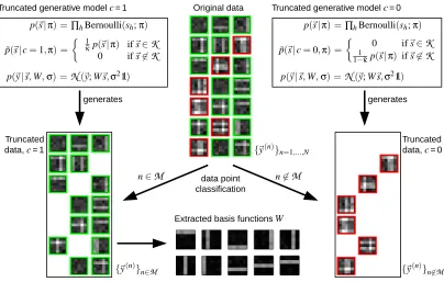
Extracted basis functionsW

Truncated data,c= 1

Truncated data,c= 0 generates generates

n∈M n6∈M

Original data Truncated generative modelc= 1

{~y(n)}n=1,...,N

Truncated generative modelc= 0

data point

˜

p(~s|c=1,π) =

1

˜

κp(~s|π) if~s∈K

0 if~s6∈K p˜(~s|c=0,π) =

0 if~s∈K

1

1−κ˜ p(~s|π) if~s6∈K

{~y(n)}n6∈M {~y(n)}n∈M

classification

p(~y|~s,W,σ) =N(~y; W~s,σ2₁₎

p(~y|~s,W,σ) =N(~y; W~s,σ2₁₎

p(~s|π) =_∏hBernoulli(sh;π) p(~s|π) =∏hBernoulli(sh;π)

Figure 1: First variational approximation: data classification. The figure shows Expectation Trun-cation (without preselection) for a concrete generative model. In this example, the gen-erative model generates data by linearly superimposing basis functions in the form of horizontal and vertical bars. Data generated by the original model contains up to ten bars chosen with a Bernoulli prior (example data points are shown in the center). Data generated by the truncated generative model with c=1 contains up to two bars (we set

K

={~s| ∑jsj≤γ}withγ=2). Data generated by the truncated generative model with

c=0 contains at least three bars. If we train the truncated generative model with c=1 on data from which data points with∑_jsj>γwere removed, we can expect to approximately recover the true generating basis functions W of the original model.

3.1 First Variational Approximation: Data Classification

As in Section 2, let us consider a generative model with a set of hidden variables denoted by~s, a set of observed variables denoted by~y, and a set of parameters denoted byΘ. Let us denote the prior distribution of the model by the (not further specified) function p(~s|Θ), and the noise distribution by the (not further specified) function p(~y|~s,Θ). To distinguish this generative model from models introduced later, it will from now on be referred to as the original generative model.

models by introducing two new prior distributions that are based on the original prior:

p(~s|c=1,Θ) =

₁

˜

κp(~s|Θ) if~s∈

K

0 if~s6∈

K

and p(~s|c=0,Θ) =

0 if~s∈

K

1

1−κ˜ p(~s|Θ) if~s6∈

K

(10)

where ˜κ=∑_~s∈K p(~s|Θ). We take the noise distribution p(~y|~s,Θ)of the new models to be identical

to the original noise distribution. We will refer to the new generative models as truncated models because their prior distributions are truncated to be zero outside of specific subsets. Note that the generation of data according to the truncated model with c=1 corresponds to generating data ac-cording to the original model while only accepting data points generated by~s∈

K

. Analogously, generating data according to the truncated model with c=0 is equivalent to generating data accord-ing to the original model while acceptaccord-ing only data points generated by~s6∈

K

. Figure 1 shows the truncated generative models and data they generate for a concrete example (a model that linearly combines bar-like generative fields; compare Section 4.1). For the example,

K

is the set of binary states~s with less or equalγnon-zero entries. In general,

K

can be any subset, however.

Let us now mix the two truncated models in Equation 10 by introducing c∈ {0,1}as additional hidden variable and by drawing c=1 with probabilityκ. The prior distribution of this mixed model is thus given by:

p(c|κ) = κc_(1−κ)1−c_{, (11)}

p(~s|c,Θ) = c ˜

κ δ(~s∈

K

) +

1−c

1−κ˜ δ(~s6∈

K

)

p(~s|Θ). (12)

where we have introducedδ(~s∈

K

) =1 if~s∈

K

and zero otherwise, andδ(~s6∈

K

) =1 if~s6∈

K

and zero otherwise. We will refer to this model as the mixed generative model. Note that the mixed model is identical to the original generative model if we chooseκ=κ˜ =∑~s∈K p(~s|Θ)as mixing

proportion. The mixed model thus contains the original model as a special case.

Now, consider a set of N data points{~y(n)}n=1,...,Ngenerated according to the original generative model. Let us maximize the likelihood of the data under the mixed model (11) and (12). If we use EM for optimization (compare Section 2), we obtain the free-energy

˜

F

(q,Θ,κ) =

∑

n

∑

c

q(n)(c ;Θold)log p(~y(n)|c,Θ) +log(κ)

∑

n

q(n)(c=1;Θold) +log(1−κ)

∑

n

q(n)(c=0;Θold) +H(q), (13)

where H(q)is the entropy w.r.t. q(n)(c;Θold)(summed over all n and c). The free-energy (13) can be optimized iteratively by maximizing q in the E-step and(Θ,κ)in the M-step. For the E-step, choos-ing the exact posterior, q(n)(c ;Θold) =p(c|~y(n),Θold_{), represents the optimal choice. Unfortunately,} it is computationally intractable in general because

p(c=1|~y(n),Θold) =∑~s∈K p(~y

(n)_,~s|Θ) ∑~sp(~y(n),~s|Θ)

(14)

reduces the free-energy (13) to:

˜

F

(q,Θ) =

≈L1(Θ)

z }| {

∑

n∈M

log p(~y(n)|c=1,Θ)+

≈L0(Θ)

z }| {

∑

n6∈M

log p(~y(n)|c=0,Θ)

+log(κ)|

M

|+log(1−κ)(N− |

M

|) +H(q). (15)

where

M

={n|q(n)(c=1 ;Θold) =1}. Note thatκcan be optimized independently ofΘbecause the first two summands in (15) only depend onΘ. As we also know its final optimal value (κ=κ˜), we will treat the mixing proportion as implicitly known.κcan thus be omitted as a parameter of the free-energy (15) and will not play a role for our further considerations.

For the data set

M

note that the best choice for q(n)(c ;Θold)under the constraint q(n)(c ;Θold)∈ {0,1}is given by the assignment q(n)(c=1 ;Θold) =1 if~y(n) was generated by class c=1 (and zero otherwise). This would amount to setting

M

to

M

opt={n|~y(n)generated by class c=1}. (16) In general this best choice can not be computed exactly. We can, however, derive tractable ap-proximations to

M

opt_{. Choosing a set}

_M

_{is equivalent to choosing a distribution q}(n)_{(c ;Θ}old_)with binary values (as an approximation to Equation 14). Any choice of

M

thus represents a variational approximation. In Appendix A.2 it is shown that one such approximation is obtained via sorting according to the denominator values in Equation 6. The selection of Ncut data points obtained in this way is thus equivalent to a variational E-step.

An interesting aspect of Equation 15 is that the first two summands take the form of two log-likelihoods. The first summand is the likelihood L1(Θ)of the truncated generative model with c=1, and the second is the likelihood L0(Θ)of the model with c=0. If

M

=

M

opt, both likelihoods are evaluated on the set of data points they can generate (see Figure 1). Considering these properties of Equation 15 the question arises how the maximum of ˜

F

(q,Θ)and the maxima of L1(Θ)and L0(Θ) are related. It could, for instance, be asked if all three functions have a maximum for the same parameter values. From the structure of the equation this can not be concluded, and, indeed, the question must be answered negatively because it can be shown that in general the maxima do not coincide. However, under assumptions that are usually fulfilled at least approximately, we can show that any global maximum of ˜

F

(q,Θ)is an approximate global maximum of L1(Θ)and of L0(Θ). A necessary condition for an approximate global maximum of L(Θ)(the likelihood of the original model) is thus a global likelihood maximum of L1(Θ) (or of L0(Θ)). The technical derivation of this observation is given in Appendix A.1.

3.2 Second Variational Approximation: Preselection

Starting point for the second variational approximation will be the likelihood L1(Θ)of the truncated generative model c=1. We have seen in the previous section (and Appendix A.1) that a global maximum in L1(Θ)is a necessary condition for an approximate global maximum of the likelihood L(Θ)of the original model. To find the maximum of L1(Θ)we optimize the lower bound

F

1(q,Θ) given by:

F

1(q,Θ) =

Q1(q,Θ)

z }| {

∑

n∈M~s

∑

∈K

q(n)(~s ;Θold) logp(~y(n)|~s,Θ)1 ˜

κp(~s|Θ)

+H(q), (17)

with∑_~s∈Kq(n)(~s ;Θold) =1.

F

1(q,Θ)is derived by a variational approximation, this time w.r.t. the hidden variables~s. The free-energy equals the likelihood L1(Θ)after each E-step if the distributions q(n)(~s ;Θold)are given by:

q(n)(~s ;Θold) = p(~s|~y(n),c=1,Θold) = p(~s|~y

(n)_,Θold₎

∑~s′_∈K p(~s′|~y(n),Θold)

δ(~s∈

K

). (18)

M-step rules can be derived by setting the derivatives of

F

₁(q,Θ)w.r.t. all parameters to zero. As the entropy term in (17) is independent ofΘif q is held fixed, we obtain

d

dΘ

F

1(q,Θ) = d

dΘQ1(q,Θ) =0 (19)

as necessary condition. The derivative _dd_Θ hereby stands for derivatives w.r.t. all the individual parameters.

Based on condition (19) we can now introduce candidate preselection as a variational approxi-mation. As described in Section 2, preselection amounts to selecting, for a given~y(n), a subset

K

_n of the state space. Section 2 gives an example of how to define the set

K

and how to construct subsets

K

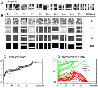
nusing selection functions. Figure 2 shows a concrete example of how a set

K

nis con-structed using selection function values

S

_h(~y(n)). In Section 4 and Appendix B different instances of selection functions can be found. More generally, we here require from the sets

K

_n that for all data points generated by~s∈

K

, they finally contain most of the posterior mass in

K

. If this applies, we obtain an approximation to the posterior q(n)in (18) given by:

˜

q(n)(~s ;Θold) = p(~s|~y

(n)_,Θold₎

∑~s′_∈K

np(~s

′_|~y(n)_,Θold₎ δ(~s∈

K

n) =

p(~s,~y(n)|Θold₎

∑~s′_∈K

np(~s

′_,~y(n)_|Θold₎ δ(~s∈

K

n). (20) Note that ˜q(n)(~s ;Θold)sums to one in

K

as

K

n⊆

K

. It thus fulfils the condition on q(n)required for (17). If preselection finds, at least finally, appropriate sets

K

_n, we obtain with (20) the necessary condition: _dd_ΘQ1(q˜,Θ)≈_dd_ΘQ1(q,Θ) =0. Parameter update rules derived from _dd_ΘQ1(q˜,Θ) =0 can therefore be expected to (at least approximately) optimize the free-energy (15) and thus L1(Θ). The update rules derived will contain expectation values (the sufficient statistics) of the formhg(~s)i_q˜(n).

If we use (20) for these expectations we obtain:

hg(~s)i_q˜(n) =

∑

~s ˜

q(n)(~s ;Θold)g(~s) =

∑

~s∈Kn

p(~s,~y(n)|Θold)g(~s)

∑

~s′_∈K

n

s9

s2

s3

s7 0 0 0 0 1 0 0 1 0 1 1

h

23 7 9

Sh ˜

q(n)(~s ;Θold)

~s

0 0 0 1 1 1 0 0

1

0 0

0 0 1 0 0 1 0 0 1 1 0

0 0 0 1 0 0 1 0 1 0 1

~y(n)

selection of

H′=4candidates

computation of selection functions

comparison

W(~s,W)

states~s∈Kn sh=0for all otherh

Figure 2: Second variational approximation: preselection. The figure illustrates how the variational approximation ˜q(n)(~s ;Θold)in Equation 20 is computed. The selection of hidden states ~s∈

K

n and the computation of ˜q(n)(~s ;Θold)are shown for the example of Figure 1 close to the optimal parameters W . Given the data point~y(n)a selection function value

S

_hfor each hidden variable h is computed. The H′ largest values are selected (H′=4 for this example). The approximation ˜q(n)(~s ;Θold)is then computed based on the combinatorics of these H′candidates (with∑_jsj≤γ=2). For the displayed data point and parameters all values of ˜q(n)(~s ;Θold)except for one lie close to zero. For visualization purposes these values have been increase in the figure.

that is, precisely expression (6) in Section 2. Expectation Truncation, introduced as an approx-imation to Equation 5, can thus been derived as a variational approxapprox-imation. Importantly, this approximation is tractable if

K

n is small. The computational gain of preselection compared to an approximation without preselection is reflected by the reduced size of

K

_n compared to

K

(see Figure 2 for an example and Appendix C for a detailed complexity analysis).

3.3 Summary and Numerical Controls

We have seen that the approximation procedure introduced in Section 2 can be derived as a vari-ational EM approach. This approach consists of two varivari-ational approximation steps: First, an approximation that assigns the data points to two classes (Section 3.1). Second, a variational step that approximates the posterior (18) by an approximate posterior (20) defined through preselection (Section 3.2). Although the derivation of ET as a variational approach requires in parts rather tech-nical steps, the final result is intuitive (see Figure 1 and Figure 2) and can be stated very compactly. Algorithm 2 summarizes all required steps of the approximation scheme.

Algorithm 2: Expectation Truncation

Preselection: select a state space volume

K

_nfor each data point~y(n)

Data classification: find a data set

M

that approximates

M

opt_{in Equation 16} E-step: compute ˜q(n)(~s ;Θold) = p(~s,~y

(n)_|Θold₎

∑~s∈Knp(~s,~y

(n)_|Θold₎ for all~y

(n)_and~s∈

_K

n

M-step: find parametersΘsuch that d

dΘ_n

∑

∈M~s∈

∑

Kn

˜

q(n)(~s ;Θold) logp(~y(n)|~s,Θ) p(~s|Θ)

∑~s′_∈K p(~s′|Θ)

=0

and it appears in the M-step equation (Algorithm 2). Because of symmetries in the usual priors for generative models, this sum can, however, be computed without summing over all~s explicitly (an example is given in the next section). Even if symmetries can not be exploited, note that the sum over~s∈

K

has to be computed at most once per EM iteration and not once per data point and per EM iteration (as it is the case for the sums over

K

_n).

Algorithm 2 summarizes ET as a variational approximation and represents a generalization of Algorithm 1. Algorithm 1 in Section 2 contains, for example, one specific way of how to select an appropriate set

K

and appropriate sets

K

n: we defined

K

based on sparseness and selected

K

_n using selection functions

S

_h. In the variational derivation of ET we, however, only specified the properties required from

K

and

K

_n. In general,

K

does not have to be defined based on a sparseness assumption and there are potentially alternative ways to define the sets

K

n. Importantly, the variational derivation of ET allows for a comparison with other variational approaches. We can thus observe that ET is qualitatively different from the standard variational approach. Concrete instances of variational EM usually approximate the exact posteriors by fully or partly factored distributions over the hidden variables (compare Jordan et al., 1999; Jaakkola, 2000; MacKay, 2003; Bishop, 2006). Such approximations become the more severe the stronger dependencies between the hidden variables in the posterior are. In the derivation of the ET approximation, no independence assumption for the posterior has been used. Strong dependencies are therefore not expected to negatively affect the approximation quality of ET. On the other hand, the ET approximations can get more severe if the approximate classification of data points becomes imprecise (first variational step), if the preselection step does not include the relevant candidates (second variational step), or if too few data points are used.

monitor the quality of the data point classification (first variational approximation) and the quality of the approximation by preselection (second variational approximation). For the first approxima-tion we compare the obtained classificaapproxima-tion with ground-truth of all data points. For the second approximation, we will monitor the differences between the exact posterior p(~s|~y(n),Θ) and the approximate posterior ˜q(n)(~s;Θ)in (20). If we evaluate the differences between these distributions using the Kullback-Leibler divergence, we obtain:

DKL(q˜(n),p) =−log(Q(n)) with Q(n) =

∑~s∈Knp(~s,~y (n)_|Θ) ∑~s′p(~s′,~y(n)|Θ)

. (21)

The preselection approximation has a high quality if for the data points in

M

the values DKL(q˜(n),p) are close to zero. For data points not in

M

the differences between the distributions should be large. For practical reasons, we have introduced the quality values Q(n)_{in (21). The values Q}(n)_measure

the percentage of the posterior probability mass concentrated in

K

n. In terms of these values the approximation quality is high if Q(n)is close to one for data points in

M

, and close to zero for data points not in

M

.

4. Training Generative Models

The approximation scheme defined and discussed in the previous sections is so far independent of the specific choice of a generative model except for the assumption of binary hidden variables. To demonstrate the applicability of the method and to investigate its properties, in this section we will apply it to a number of different generative models. The investigated models are all multiple-cause models that require tractable approximations. The three major classes investigated here are non-negative matrix factorization (NMF; Section 4.1), maximal causes analysis (MCA; Section 4.2), and a sparse-coding-like model termed LinCA (Section 4.3). For all these models we will assume independent hidden variables distributed according to a Bernoulli prior:

p(~s|π) = H

∏

h=1

p(sh|π), p(sh|π) =πsh(1−π)1−sh, (22) whereπ∈[0,1]parameterizes the sparseness of the distribution. For binary hidden variables the Bernoulli prior represents the most straightforward choice (compare, e.g., Berkes et al., 2009; L¨ucke and Sahani, 2008). Given the prior (22) the expected number of data points generated by less or equalγcauses is given by:

N≤γ =N

∑

~s,|~s|≤γ

p(~s|π) =N γ

∑

γ′₌₀

H

γ′

πγ′

(1−π)H−γ′

. (23)

N≤γis required to find the set of Ncutdata points

M

considered for a parameter update, and Equa-tion 23 shows that this number is tractably computable. For all generative models we will use ET as described in Section 2 and Algorithm 1. That is, we will use a set

K

that constrains the number of simultaneously active causes, and use selection functions

S

hto obtain sets

K

n.

4.1 Non-negative Matrix Factorization (NMF)

The first generative model considered uses prior (22) and combines the generative fields ~

that the probability of a data vector~y given~s is defined by:

p(~y|~s,Θ) = D

∏

d=1

p(yd|Wd(~s,W),σ), p(yd|w,σ) =

N

(yd; w,σ2) (24) with Wd(~s,W) =

∑

h

Wdhsh, (25)

with W ∈R

D×H_.

_N

_(y

d; w,σ2)is a scalar Gaussian density function with mean w and varianceσ2. The introduction of W will turn out to be convenient for the analytical treatment below. Note that we otherwise could have written p(~y|~s,Θ) =

N

(~y;W~s,σ2_1).

We then use (24) to compute the update equation (the M-step) for the weight matrix W as described in Section 2. The update equation is gained from the necessary condition for an optimum of the free-energy in (2). The W -update is consequently a function of the sufficient statisticsh~siT_q(n)

and~s~sT_q(n). Following Section 2, these expectation values are approximated by using (6) instead

of the exact sufficient statistics (5), that is, we use a subset of cause combinations as selected by the truncation approach. Furthermore, we sum only over the Ncutdata points in

M

as explained at the end of Section 2. The update equation is then given by:

W =

∑

n∈M

~y(n)h~siT_q(n) !

∑

n′_∈M

~s~sT_q(n′) !−1

. (26)

Note that the equation can consistently be gained from the necessary condition for a free-energy optimum in Equation 19 (see M-step of Algorithm 2).

Equations 24 to 26 are valid irrespective of the sign of the entries of the generative fields and the input data. Generative models corresponding to the class of non-negative Matrix Factorization (NMF) methods are based on a linear combination of generative fields but rely on non-negative data points and generative fields. In Equation 26, non-negativity can be ensured for the generative fields by clamping small appearing weights at zero.

A more direct way to ensure non-negativity for the parameters of the model defined by (22) and (24) is to rely on convergence proofs similar to those used for classical NMF (Lee and Seung, 2001), that is, to ensure non-negativity by deriving a multiplicative update rule for the generative fields. For the EM algorithm used as a basis for ET, it can be shown that the parameter-free update rule

~

Wh←W~h⊙

h~y shiET

∑h′W~_h′hs_h′s_hi

ET

(27)

provides monotonic convergence towards the M-step solution of the generative fields, where we have introduced the ET-averaging

hf(~y,sh)iET:=

∑

n∈M~s∈

∑

Kn

p(~s|~y(n),W)f(~y(n),sh) =

∑

n∈M

D

f(~y(n),sh)

E

q(n) .

Equation 27 corresponds to a partial M-step of ET-NMF (‘Expectation-Truncation-NMF’). In sim-ulations, it is therefore applied iteratively with 20 partial M-steps after each E-step.

chosen to ensure convergence” (Lee and Seung, 2001). A thorough derivation of the update Equa-tion 27 and its relaEqua-tion to the classical NMF algorithm known from the literature can be found in Appendix D.

The E-step of ET-NMF is based on the truncated expectation values (6) to calculate the averaged quantities in the W update equations according to

h~y shiET=

∑

n∈M

~y(n)hshiq(n) and hsh′s_hi

ET=

∑

n∈M

hsh′s_hi_q(n)

so that the sufficient statistics of the ET-NMF model that have to be computed for the M-step will be given by the first and second order momentshshiq(n) andhsh′s_hi_q(n) of the (approximate) posterior.

For our generatively formulated version of NMF with M-step equations (26) or (27) we can now apply ET as described in Section 2. We ran the ET-NMF algorithm with both M-step versions (26) and (27) and observed, at least for the data used, a qualitatively and quantitatively comparable behavior. Note that the probability density p(~y|Θ)of the model is invariant under the exchange of any two generative fields (or basis functions),W~h→W~h′, because of symmetric priors. By the

def-inition of the truncated generative models (Section 3), it can instantly be seen that their probability densities p(~y|c=1,Θ)and p(~y|c=0,Θ)are also invariant under these transformations (the same will apply for the other models considered).

As indicated, the sufficient statistics for ET-NMF are given by the first and second order mo-ments,hshiq(n) andhsh′s_hi_q(n), of the exact posterior; to find approximations to these intractable

ex-pectation values we first have to find appropriate selection functions

S

_h. A natural starting point for finding such functions is to consider the joint probability p(sh=1,~y(n)|Θ) =∑~s(sh=1)p(~s,~y

(n)_|Θ).

If we knew that the joint probability was small for a given h, we would know that the sum over all~s in (6) which contains~s with sh=1 is small as well. Furthermore, note that for a given data point the joint represents the part of p(sh=1|~y(n),Θ)which depends on h, p(sh=1|~y(n),Θ) = p(sh=1,~y

(n)_|Θ)

p(~y(n)_|Θ) .

p(sh=1|~y(n),Θ), on the other hand, directly reports the probability of unit h to have contributed to the data point. It could thus be regarded as the optimal selection function. Unfortunately, neither p(sh=1,~y(n)|Θ) nor p(sh=1|~y(n),Θ)are computationally tractable and, thus, neither function fulfils one of the properties demanded from a selection function. Therefore, we will compute an upper bound of p(sh=1,~y(n)|Θ) which is tractable and still serves well in selecting a subset of hidden units that can explain a given~y(n). Let us for this purpose consider the data point dependent weight matrix defined by: W_dhub :=W_dhub(~y(n),W) =max{y_d(n),Wdh} andW~hub:= W1hub, . . . ,WDhub

T , where ‘ub’ refers to ‘upper bound’. This formal definition of Wub allows for a compact notation of an upper bound of p(sh=1,~y(n)|Θ). Because of the non-negativity of the entries in W and the mono-modality of the Gaussian distribution w.r.t. the mean, we can show (see Appendix B for details):

p(sh=1,~y(n)|Θ) =

∑

~s(sh=1)

p(~y(n)|Wd(~s,W),σ)p(~s|π) ≤ πp(~y(n)|W~hub,σ) =:

S

h(~y(n)). (28)

the M-step in (27) or (26) represents the learning algorithm for the NMF generative model defined by (22), (24) and (25) with non-negativity constraint.

In addition we add after each M-step a small parameter noise to the basis vectors W (iid Gaus-sian, standard deviation 0.05) and we use a standard relaxation scheme in order to avoid local optima of the potentially multi-modal likelihood landscape. Annealing (see, e.g., Ueda and Nakano, 1998; Sahani, 1999) amounts to the replacements:(1/σ2_)→(β/σ2_),π→πβ_{and(1−π)→(1−π)}β_{. The} constantβis an inverse ‘temperature’,β=1/T , where T is decreased from a high value Tinit_{to a} value Tfinalequal or close to one.

4.1.1 EXPERIMENTS - ARTIFICIALDATA

Let us consider data as displayed in Figure 3A. That is, we consider hidden causes in the form of horizontal and vertical bars (five pixels each) on a 5×5 grid. Each bar appears with probability ₁₀2 such that there are on average two bars per data point. We use N=500 data points. The grey-value of a bar is taken to be 10, background pixels are zero. The bars superimpose linearly (pixel values in regions of overlap are 20) and are subject to Gaussian noise with standard deviationσ=2.0. Data as in Figure 3A are well-suited to study the functioning of the approximation scheme because we know the underlying generating process and have ground-truth for each data point. We will later use this knowledge to illustrate the influence of each data point on the update of the model parameters. For this reason data points such as displayed in Figure 3A or versions without noise are frequently used in the recent literature (see, e.g., Hinton et al., 1995; Hoyer, 2002; Spratling, 2006).

The model which is applied to the data uses H =10 hidden units and D=25 observed units. The entries of W are initialized by drawing iid from a Gaussian distribution with a mean of 4 and a standard deviation of 4₃. The standard deviation of the generative model is set toσ=2.0 and the value ofπis set to ₁₀2. Small deviations from these values did not have significantly negative effects on the algorithms performance in extracting data components. Figure 4B shows the cooling sched-ule for annealing. We linearly decrease T from Tinit=13 to Tfinal=1 during 100 EM-iterations (including ten initial iterations at Tinit and twenty final iterations at Tfinal). Figure 3B shows a typical time-course of the parameters W if trained as described above. As approximation param-eters we used H′=5 andγ=3. Although approximate EM schemes do in general not guarantee the increase of the data likelihood, we find that the learning algorithm increases the likelihood to values close to the one for the generating parameters (dashed horizontal line in Figure 4A). This behavior is reflected by the convergence of the model parameters to values close to the generating ones (compare Figure 3). In most trials the parameters converged to approximately optimal values relatively early but in some trials they converged relatively late during learning (compare likelihood values in Figure 4A). We ran 50 trials with 50 different sets of data points generated as described above. The algorithm extracted all bars in all of the trials (see Appendix E for measurement de-tails). To quantify the quality of parameter reconstruction we computed, for each trial, the mean absolute error (MAE) between the obtained generative fields,W~h, and the corresponding generating causes: MAE= 1

HD∑hd|Wdh−W_dhgen′ |where W

gen

dh′ denotes the cause represented byW~h (compare Appendix E). For all trials the MAE was smaller than 0.24 with a mean of 0.20 (note that pixels of bars were set to 10.0 and background to zero).

B

A

Wd5 Wd4 Wd3 Wd2

Wd1 Wd6 Wd7 Wd8 Wd9 Wd10 iterations

Data points

0

5

10

100 20

Figure 3: A 14 data points of the linear bars test with Gaussian noise. B Time course of the gen-erative fields W of the NMF-like gengen-erative model if Expectation Truncation is used for learning.

single bars in the four remaining cases. All successful trials had a MAE of below 0.20 with a mean MAE of 0.05. Parameter recovery was more precise than in the previous trial series because of the non-noisy data. A higher initial temperature or a longer cooling increased reliability to values close to 100% for this data. E.g., when we used Tinit=15 and stretched the cooling schedule in Figure 4B to 200 iterations, the algorithm found all bars in all of 50 trials. Likewise, increasing the number of data points increased reliability (>94% reliability for N>1000 data points with T =13 and 100 iterations cooling).

High reliability (i.e., a high probability to extract all causes) in this linear bars test has also been observed for other learning algorithms (see, e.g., algorithms investigated in Spratling, 2006). Note, however, that the standard bars benchmark test (F¨oldi´ak, 1990) uses non-linearly overlapping bars (we will come to the standard version of the bars test in the next section). For the presented NMF algorithms we have (as is usual in the literature) only inferred the parameters W . In our generative setting it is in principle also possible to learn the model parametersσandπ(compare L¨ucke and Sahani, 2008). However, for comparison with other approaches and for brevity, we focused on W .

iterations iterations

data points iterations

20 40 60

20 40 60 1 100 200

D

-100 -60 -40 -20

-80 log_zZ˜

o

1

Q(n)

C

1

B

T

1

A

-5

L 104

-7 -6

-4 10

5

0 ₅₀

0.5

0.0

Likelihood values Cooling schedule

Data point classification Approximation quality

Tinit

Tfinal

data points generated by≤γcauses data points generated

by≤γcauses

data points generated by>γcauses

data points generated by>γcauses

Ncut

Figure 4: A Data likelihood during ten trials using the same set of N =500 data points but dif-ferent random initializations. The likelihood value that results from using the generating parameters is marked by the dashed horizontal line. B Cooling schedule during learning. C Approximation qualities Q(n) of 40 data points during learning. Twenty of the data points were generated by≤γcauses (bright green lines) and the other twenty by more thanγcauses (dark red lines). D Sorted values of the sums ˜Z=∑~s∈Knp(~s,~y

(n)_{|Θ)at the}

end of learning. Bright green bars were used to mark the data points generated by≤γ

causes, dark red bars to mark data points generated by more thanγcauses. The Ncutdata points left of the black vertical line were used in the final M-steps.

or equalγ=3 active causes. For other trials, the values Q(n)show the same qualitative behavior. However, the exact time-courses can differ quantitatively from trial to trial.

Note that the poorly approximated data points do finally not negatively affect the parameter updates because they are not taken into account for the M-step. This is illustrated in Figure 4D which shows the logarithms of the sum ˜Z=∑_~s∈Knp(~s,~y

(n)_{|Θ)at the end of learning and for each}

of the N =500 data points used (divided by a common factor zo). Bright green bars display the values of all data points generated by less or equalγcauses, dark red bars display the values of all other data points. The data points are ordered descendingly. According to the approximation used (see Section 2 resp. Equation 23), we only consider the Ncutdata points left of the black bar, that is, we finally only use data points with quality values Q(n)_{close to one. The relation of the quality}

4.1.2 EXPERIMENTS - MOREREALISTICDATA

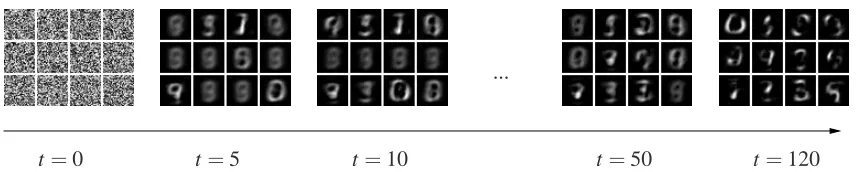
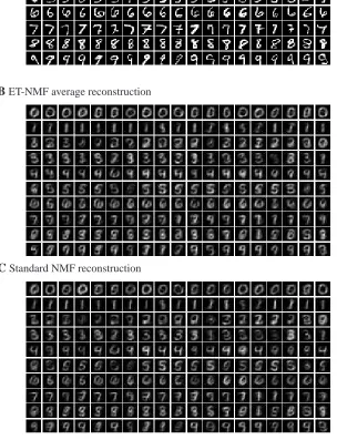
As a second example, we applied the learning algorithm to gray-valued images of the postal digits database MNIST (http://yann.lecun.com/exdb/mnist/). This data is frequently used in the NMF literature, which makes it well suited as a means for comparison of our algorithm to standard NMF approaches. Note that we do not have ground-truth about the hidden components in this case.

t=0 t=5 t=10

...

t=50 t=120

Figure 5: Resulting basis vectorsW~hfor the MNIST database. The probabilistic version of NMF trained with ET converges to a parts-based decomposition.

Figure 5 shows the application of the algorithm using H =12 hidden variables and approxi-mation parameters for ET set to H′=10 andγ=5. The prior parameter was set toπ=0.3 such that three to four of the 12 latent variables do explain a data point on average. The noise parameter

σin (24) was set to σ=0.73 after screening through values between zero and one. The dimen-sionality of each data point is D=28×28 and we used a subset of N=1000 data points, some of which are shown in Figure 6A. We linearly decreased the temperature as in Figure 4B but used a slightly longer learning time (120 iterations) to provide more time for convergence. In Figure 5 the time course of W displayed as basis vector sets is shown. As can be observed, the parameters W converge to basis vectors that represent digit parts.

To assess the quality of the basis vectors and for comparison with standard NMF, we show average reconstructions of probabilistic NMF and standard NMF in Figure 6. In Figure 6B it can be observed that already for the small subset of 12 basis vectors in Figure 5 the reconstructions match the inputs in Figure 6A relatively well. Despite the constraint to binary hidden variables in our generative version of NMF, the resulting reconstructions are very similar to those of standard NMF as shown in Figure 6C. For these data, the overall average reconstruction error, _ND1 ∑_n||~y(n)₋ ∑hW~hhshi_q(n)||2, of the generative version is less than 5% larger than the reconstruction error of

standard NMF.

4.2 Maximal Causes Analysis (MCA)

The second generative model we consider was suggested to extract the hidden causes from data whose components combine non-linearly. It uses a maximum rule in the place where NMF, sparse coding (Olshausen and Field, 1996), independent component analysis (ICA; Comon, 1994) and many other methods assume a linear superposition of hidden components:

p(~y|~s,W) = D

∏

d=1

p(yd|Wd(~s,W),σ), p(yd|w) =

N

(yd; w,σ2) (29) with Wd(~s,W) =max

ADigit data used for testing the ET-version of NMF

BET-NMF average reconstruction

CStandard NMF reconstruction

where we have used a Gaussian noise model with w as a place-hoder for Wd(~s,W)(note the dif-ference to Poisson noise used by L¨ucke and Sahani, 2008). For the activities of the binary hidden variables shwe use the same prior as for the NMF model in Section 4.1 (see Equation 22). As in the previous model, the weight matrix W ∈R

D×H_{parameterizes the influence of the hidden causes on}

the distribution of~y. The function Wd(~s,W)in (29) gives the effective weight on yd, resulting from a particular instance of the state vector~s. An update rule for the weight matrix W of this model was derived in L¨ucke and Sahani (2008) and is given by:

Wdh =

∑

n∈M

A

ρ_dh(~s,W)_q(n)y (n)

d

∑

n∈M

A

ρ_dh(~s,W)_q(n)

, where

A

ρ_dh(~s,W) =

_∂

∂Wdh

Wρ_d(~s,W)

(30)

Wρ_d(~s,W) = H

∑

h=1

(shWdh)ρ

!1

ρ

. (31)

The parameterρcontrols the nonlinearity and is increased to large values during learning. Again, the entries in W are non-negative. To derive a selection function we can therefore apply the same arguments as for NMF and thus arrive at the very same functions

S

_has given in Equation 28. The selection function (28), M-step equations (30) and (31), and the E-step approximation described in Section 2 represent a full learning algorithm for the extraction of non-linearly combining compo-nents, which will be referred to as MCAET.

4.2.1 EXPERIMENTS - ARTIFICIALDATA

To study the properties of MCAET let us first apply it to data with ground-truth. A well-suited type of data for the algorithm is the so-called bars test introduced by F¨oldi´ak (1990). The bars test has become a standard benchmark for component extraction algorithms (see, e.g., Saund, 1995; Dayan and Zemel, 1995; Hochreiter and Schmidhuber, 1999; Charles et al., 2002; L¨ucke and von der Malsburg, 2004; Spratling, 2006; Butko and Triesch, 2007; L¨ucke and Sahani, 2008) and thus allows for quantitative comparison with other systems. To generate data according to the bars test we use the same parameter settings as for the artificial data in Figure 3A, that is, D=5×5, bars pixel value 10 and other pixels zero, Gaussian generating noise with standard deviation 2.0, and the probability for each bar to occur is ₁₀2. In contrast to the data used in the experiment of Figure 3, however, the standard form of the bars test uses a non-linear superposition of the causes (overlapping bar regions have pixel values 10 instead of 20 for NMF). Figure 7A shows a random selection of 12 of the N=500 data points used.

Wd5

Wd4

Wd3

Wd2

Wd1 Wd6 Wd7 Wd9 Wd10

0

10

40

100

Wd8

B

Data points

A

iterations

20 40 60 1 20 40 60

Q(n)

D

0.5

0.0

Approximation quality

iterations 1

C

L 104

Likelihood values

iterations -6

-5 -4

≤γcauses >γcauses

Figure 7: A Example data of a bars test with D=5×5 and additive Gaussian noise. B Time course of W for the MCA model trained with ET. C Likelihood values for ten trials with the same set of training patterns and different initial conditions for each trial. D Time course of the quality values of 40 data points during one trial. Values are plotted for twenty randomly selected data points generated by less or equalγcauses (bright green lines) and twenty randomly selected data points generated by greater thanγcauses (dark red lines).

Figure 7B shows a typical time course of W during learning. Figure 7C shows time courses of the data likelihood for ten different runs using the same data set. The behavior of the likeli-hood values results from the specific form of annealing which includes the annealed nonlinearity in Equation 31. In Figure 7D typical time courses for the quality values Q(n)(Equation 21) for 40 data points are shown. For the 20 data points which were generated by ≤γcauses (bright green lines) the quality values increased to one. For the data points generated by >γcauses (dark red lines) the quality values finally decreased to zero. As for NMF, only the data points which were well approximated were finally taken into account for learning.

MAE of 0.29 (bars had value 10). We observed that the convergence to local optima in 8% of the trials was mainly due to effects of finite sample size. When we ran 100 trials using the same parameters but N=2000 data points instead of N=500, the algorithm extracted all bars in all trials. For comparison with other methods, we ran additional trials using the same parameters for bars generation but with Gaussian noise for data pixels set to variance zero. This version of the bars test is presumably the one most commonly used in the literature (e.g., Saund, 1995; Dayan and Zemel, 1995; Hochreiter and Schmidhuber, 1999; L¨ucke and Sahani, 2008). In 41 of the 50 trials MCAETextracted all bars (82% reliability) and found 9 of 10 bars in the other nine trials. Again, reconstruction of the generating parameters in the successful trials was high with a maximal MAE of 0.14 and a mean MAE of 0.05. Also for the non-noisy bars test, reliability of the algorithm increased when we increased the sample size. For instance, we obtained reliabilities of more than 90% for N larger than about 2000. With N =10 000 and slower cooling (same cooling schedule as in Figure 4B but stretched to 200 iterations), the algorithm found all bars in all of the 50 trials. Achieving close to 100% reliability is thus more difficult for non-noisy bars.1

In earlier work, generative modelling approaches to the bars test merely achieved relatively low reliability values. For instance, the model of Saund (1995) achieved 27% reliability, and the model of Dayan and Zemel (1995) (although trained without overlapping bars) achieved 69%. Approaches such as PCA or ICA that assume linear superposition have been reported to fail in this task (see Hochreiter and Schmidhuber, 1999). Other objective function approaches and different types of neural network approaches (e.g., Charles et al., 2002; L¨ucke and von der Malsburg, 2004; Spratling, 2006, and references therein) have been more successful in terms of reliability. They do, however, often use hidden assumptions and constraints which make an objective comparison difficult (see, e.g., Spratling, 2006, or L¨ucke and Sahani, 2008, for discussions). The more recently suggested approach of MCA (L¨ucke and Sahani, 2008) represents a fully generatively interpretable approach which achieves high reliability values. The unrestricted version of MCA3extracts all bars in 90% of the trials with noisy bars (with Poisson noise) and in 81% of the cases for the noiseless bars. MCAETslightly improves on these results with 92% vs. 90% for noisy bars and 82% vs. 81% in the non-noisy case (experiments with N=500). If more data points are used, MCAETshows close to 100% reliability (50 of 50 trials successful, see above).

Other than the standard bars test, there has recently been an increasing interest in bars with more pronounced overlap. We therefore used a version of the bars test as suggested by L¨ucke (2004). For this data, bars of the same orientation can overlap (two neighboring vertical bars are not disjoint but overlap). For the test we adopted the same parameter setting for such input as used by Spratling (2006) and L¨ucke and Sahani (2008), that is, N=400 example patterns, 16 bars, D=9×9, bars appear with probability ₁₆2, and number of hidden units is H=32. Bars are two pixels wide such that parallel neighboring bars have a one pixel wide region of overlap. Figure 8A shows some examples of the data points used. We applied MCAETto the data using the same parameters as for the standard bars test except of a higher initial temperature (T =23) and longer cooling time (the cooling schedule in Figure 4B was stretched by a factor four to 400 iterations). In 21 of the 25 trials the system extracted all bars (see Figure 8B). In four trials 15 of the 16 bars were represented. The average number of extracted bars was thus 15.84. In all the successful trials, reconstruction of the generating parameters was high with a maximal MAE of 0.05 and a mean MAE of 0.04 (bars have

A

B

Figure 8: A Selection of 14 data points of a bars test with increased overlap. B Typical parameters W after learning if twice as many hidden units as bars are used. The supernumerous units are used to represent composite patterns.

value 10). As for the standard bars test we found that convergence to local optima was caused by effects of the finite sample size. When we repeated the experiment with the same generating and model parameters but with N=800 instead of N=400 data points, the algorithm extracted all bars in all of 50 trials (mean number of bars extracted equal to 16.0). In work by Spratling (2006) state-of-the-art systems were quantitatively compared using the mean number of extracted bars. From the evaluated systems only few achieved values close or equal to the optimal value of 16 for N=400. From the systems with high values, many required additional constraints on the parameters (e.g., constrained forms of NMF) that had to be set by hand (see Spratling, 2006; L¨ucke and Sahani, 2008, for discussions).

In general, the component extraction performance of MCAETon the different bars test tasks is similar to the performance of MCA3 suggested by L¨ucke and Sahani, 2008. In terms of computa-tional cost, MCAETrepresents a substantial improvement, however (even compared to R-MCA2, a constrained form of MCA; see L¨ucke and Sahani, 2008). This allows for applications with large H as demonstrated, for example, in the following section.

4.2.2 EXPERIMENTS - MOREREALISTICDATA

As an example for an application to more realistic data, we applied MCAET to visual data in the form of image patches. We used the same image, Figure 9A, as in work by L¨ucke and Sahani (2008) to allow for a comparison. We randomly selected N=40 000 patches of 10×10 pixels as data points (see Figure 9D for ten examples). The data points were globally scaled to lie in the interval[0,10]. However, just very few pixels had values close to 10 after scaling. The mean pixel value was 1.6 and thus smaller than for the bars test. We therefore used a smaller assumed Gaussian noise for the model (standard deviation σ=1.0 instead of σ=2.0) and started cooling at a lower temperature of Tinit=4.0. Also the small noise term on the model parameters was scaled down (0.01 instead of 0.05). During learning, we cooled for 400 iterations (cooling schedule of Figure 4B stretched by a factor four) and allowed for additional 400 iterations at Tfinal to guarantee full convergence (although changes after iteration 400 were small).

Original image

A

E

Generated patches

D

Training patches

B

LearnedW forH=50

C

LearnedW forH=100

Figure 9: Application to visual data. A The 250-by-250 pixel image used as basis for the experi-ment. The image is taken from the van Hateren database of natural images (brightened for visualization). B ParametersW~h= (Wh1, . . . ,WhD)T of the MCA generative model with

H=50 trained by ET with H′=5 andγ=3. C ParametersW~h of MCA with H=100 (H′ =5 and γ=3). D A selection of 10 typical training patches. E Ten examples of patches generated according to the MCA generative model using the generative fields in C. To reduce the apparent noise level, the patches were generated with a smallerσthan for training.

extracted generative fields thus resemble the structure of the training patches (Figure 9E). Note that the components of the data (e.g., images of grass blades and stems) superimpose non-linearly which motivated the application of MCA.