Improved-Coverage Preserving Clustering Protocol in Wireless Sensor Network

Improved-Coverage Preserving Clustering Protocol in Wireless Sensor

Networks

Manju

*

, Satish Chand,

Bijender Kumar

Netaji Subhash Institute of Technology, Sector-3, Dwarka, New Delhi, 110078, India

Received 13 November 2015; received in revised form 15 December 2015; accepted 19 January 2016

Abstract

Coverage maintenance for longer period is crucial problem in wireless sensor network (WSNs) due to limited

inbuilt battery in sensors. Coverage maintenance can be prolonged by using the network energy efficiently, which can

be done by keeping sufficient number of sensors in sensor covers. There has been discussed a Coverage-Preserving

Clustering Protocol (CPCP) to increase the network lifetime in clustered WSNs. It selects sensors for various roles

such as cluster heads and sensor cover members by considering various coverage aware cost metrics. In this paper, we

propose a new heuristic called Improved-Coverage-Preserving Clustering Protocol (I-CPCP) to maximize the total

network lifetime. In our proposed method, minimal numbers of sensor are selected to construct a sensor covers based

on various coverage aware cost metrics. These cost metrics are evaluated by using residual energy of a sensor and

their coverage. The simulation results show that our method has longer network lifetime as compared to generic

CPCP.

Keywords: sensor networks, energy-efficiency, clustering, network lifetime, coverage

1.

Introduction

Wireless sensor network (WSNs) aims to provide monitoring (called coverage) services in many areas [1]. In coverage

problems, the objective is to keep all the points of interest within the sensing range of at least one sensor node for maximum

possible time. There are many works [2-5] in this area which aims to achieve full coverage through various energy based

heuristic approaches. In all above works, it has been shown that instead of activating all the sensors at a time, it is better to

activate a subset of sensors (called sensor cover) which covers all the points of interest. After generating maximum possible

cover sets, the next phase is to communicate the data collected by these sensor covers to the base station (BS) where further

processing is to be done. In large sensor network, the maintenance of centralize processing is not performing well specially,

when it comes to the quality and throughput requirement. Therefore, it is better to design distributed network where each node

is part of processing (instead of central processor), thus, they can spread the workload out more evenly than the centralized

algorithm [6]. To apply distributed approach, the whole networks to be divided into small groups based on density,

neighbourhood, residual energy or many other parameters of interest. Recently, clustering is one of the best ways so far for

designing scalable and energy-efficient distributed sensor networks [7]. Efficient utilization of clusters reduces the

communication overhead and interference among the sensor nodes, thereby decreasing the energy consumption for overall

network architecture. Research community has widely pursue clustering over the last few years which leads to the appearance of

a great number of application-oriented customized clustering protocols [8–9]. When applying clustering, all the nodes deployed

in the network organize themselves into local groups called clusters, where only one node among each group is acting as the

cluster head. All non-cluster-head nodes used to transmit their information to their cluster heads. Due to this, some neighbouring

sensor nodes may send redundant data at the cluster head node which lead to unavoidable energy consumption in energy scared

sensor networks. To avoid this problem, the cluster head nodes perform local aggregation on the received information and

forward it to the remote base station where final processing is to be performed. Local data aggregation at the cluster heads can

significantly reduce the total amount of data to be sent to the base station thus reducing energy consumption in transmitting data.

This in turn results in longer network lifetime.

Lots of work has been done in the area of coverage problems as well as on clustering in WSNs. But, there are very few

works [10-11, 23] that dealt with both the problems (coverage problems and clustering techniques) in the wireless sensor

networks at the same time. Therefore, in this paper, our main focus is to provide coverage for longer period in clustered WSNs.

The rest of the paper is organized as follows: related work on the coverage and clustered network is given in section 2. Section

3 discusses the various coverage aware cost metrics which are further used to decide various roles of sensors. Section 4

describes the proposed heuristic called Improved-Coverage-Preserving Clustering Protocol (I-CPCP) to maximize the total

network lifetime. Section 5 gives a series of simulation results to claim the quality of proposed method. Conclusion is given in

section 6 of the paper.

2.

Related Work

Several studies on energy-efficient coverage have been conducted in the field of wireless sensor networks. Here our main

discussion is on two basic problems: coverage problems and efficient use of total network energy. Coverage problems deal with

prolonging the total coverage for maximum possible time. Since the sensors in WSNs have limited available batteries which is

not rechargeable or cannot be replaced [1], it is very essential to utilize the network energy very efficiently. The efficient

utilization of the network energy is generally done through clustering. Following sections discuss related work of the coverage

and clustering in wireless sensor network.

2.1 Coverage

The coverage problem in wireless sensor networks is an important area due to several applications including health care,

national security, environmental monitoring and surveillances [1]. There has been some works [2-5] that address the coverage

problem in WSNs. In these works, the basic objective is to activate a subset of sensors (called sensor cover) based on various

criteria like, residual energy of nodes, number of 1-hop neighbour nodes etc. One of the known variant of coverage problem i.e.

target coverage problem which has been solved by Cardei and Du [2] where disjoint sensor covers are generated such that every

target point is completely covered by each cover. They proved that the disjoint sensor set problem is NP-Complete problem.

This problem is further addressed by Cardei,Thai, Li, and Wu [3] in which the sensor covers need not to be disjoint, that is, a

sensor can be a member of more than one sensor cover (non-disjoint set). They used greedy heuristic to generate sensor cover by

giving priority to those sensors covering the critical target (covered by least number of sensors) and also those covering

maximum number of uncovered targets. Mini, Siba and Samrat [4] propose another algorithm for target coverage problem

where a weighted coverage is calculated for each sensor. To select sensor in a cover, sensor with more weights are given priority.

In many QoS based surveillance applications, it is all time necessary that particular area should be covered by at least Q-number

of sensors. It is generally used when there is a very high probability of a node failure or the data collected by the sensors with

large amount of noise. Manju and Arun [5] proposed an energy based heuristic to solve target Coverage problem where sensor

22] is also reported as NP-Complete problem. To address the impact of standby mode and energy consumption in peak hours,

Collotta and Giovanni [26] address a completely new approach called information and communication technologies (ICT). The

ICT ensures energy management in smart homes which combines a wireless network based on Bluetooth Low Energy (BLE) for

communication among home appliances, with the help of home energy management (HEM) scheme.

2.2 Clustering

As discussed in section 1, centralized communication does not perform well when deployed networks size grows

exponentially. Distributed network design can resolve this problem in energy-efficient way. As far as distributed network design

is considered, clustering is the best way to design distributed network architecture.

LEACH [12] is one of the first classical clustering protocols in WSNs which selects cluster heads dynamically and

frequently by a round mechanism and it allows different nodes to become cluster heads at each round. However, this protocol

cannot guarantee good cluster distribution and require strict time synchronization. PEGASIS [13] is an extension of LEACH, in

which all nodes are organized into a chain and each node only transmits data to its nearest neighbour. Compared to LEACH,

PEGASIS reduces the energy consumption of the nodes, but the data delay is significantly high and is proved to be unsuitable

for large-sized networks. The HEED clustering protocol [14] uses a hybrid criterion for cluster head selection, which considers

the residual energy of each node and a secondary parameter, such as the node’s proximity to its neighbours or the number of its

neighbours. HEED plays a great role in reducing the energy consumption of the nodes and enhancing the network lifetime.

HEED and LEACH require re-clustering after a period of time (called round), which causes extra energy consumption.

Therefore, to resolve this problem, the generic weight-based clustering algorithm (called Weighted Clustering Algorithm

(WCA)) [8] is proposed where each sensor associated with some weight is good examples of genetic clustering. In WCA

approach, weight is calculated from a sensor’s local properties, such as speed, node degree, coverage and residual energy.

Cluster heads are selected from those nodes that have the highest weights among their neighbours. Quin and Roger [16] discuss

a Voting based Clustering Algorithm (VCA) which performs some voting criteria to select cluster head. VCA can generate

fewer clusters and a longer lifetime than clustering algorithms discussed in [12-14]. To elect a cluster head, VCA basically

perform voting scheme where each sensor can get vote only from its neighbour sensors. So, nodes with more neighbours tend to

receive more votes. Thus, cluster heads are likely to be those high-degree nodes. Most of the clustering algorithms like LEACH,

PEGASIS and HEED [12-14] have been designed for homogenous network and they perform poorly in heterogeneous

environment. There are few works which discuss heterogeneous network. In [17], Stable Election Protocol (SEP) is discussed

for a two level heterogeneous network, which includes two types of nodes according to the initial energy, i.e. the advanced

nodes and normal nodes. It selects cluster head based on the residual energy of node and weighted probability. Kumar, Aseri

and Patel [18] discuss an energy-efficient heterogeneous cluster (EEHC) protocol for three-level heterogeneous WSNs whose

nodes are divided into three types, i.e., super, advanced and normal nodes. It selects cluster heads using the node’s energy after

dividing by the average networks residual energy and weighted probability. In [19] Hong, Li and Zhang discuss a heuristic for

multilevel heterogeneous wireless sensor networks which is known as EDCS (Efficient and Dynamic Clustering Scheme). It

calculates some weighted probability (based on remaining energy) of node to decide cluster heads.

In order to save energy consumption, Jihwan Hyang-Won and Song [24] proposed a Traffic-aware energy-saving (TAES)

base station sleeping and clustering approach where network energy is saved by putting BSs off when network capacity is

excessive compared to traffic demand. Apart from that, they also addressed a new optimal clustering method that has

polynomial complexity. To provide secure data and communication in clustered wireless sensor networks, Seung-Hyun,

(CL-EKM) for dynamic WSN. It ensures forward and backward key secrecy at the moment a node leave or joins a cluster. Due

to the severe energy constraints, hardware crash, software bugs and environmental risks, the network reliability should be on

priority as nodes. Therefore, in order to provide fault tolerant network, Venkatesh and Mehata [23] discussed a different

approach for clustering and optimal coverage of tracking multiple objects in WSNs. They proposed an improved K-means

clustering algorithm with simulated annealing technique. The discussed method finds optimal set of sensor nodes for covering

moving targets and recover from fault as soon as possible so that target detection won’t be disrupted. Another security based

method is discussed in [27] where a highly secure authentication mechanism is proposed in order to provide secure

communication between deployed nodes with gateway nodes.

As discussed in this section, there is lots of work done on coverage [4, 22, 28] and clustering [19, 29] separately, but there

are very few works which deals with both the issues collectively [10, 11]. Authors in [4] consider energy as the prime criteria to

find cover set while in [22], both coverage and energy are considered to generate sensor covers. In [28], a hybrid approach

based on genetic algorithm is used to find cover set for partial coverage. In order to provide clustering in WSN, Authors in [19]

discussed a new approach which also considers heterogeneity in terms of energy in the sensor networks. Similarly, in [29] a new

self-configurable clustering mechanism is presented which periodically check for cluster heads failure and replace these failed

CHs with newly elected nodes so that the network activity won’t interrupt. As we said earlier too, these methods do not take

coverage and clustering into account collectively. Therefore, in this paper, we consider only those works which provide

coverage and clustering both in the sensor network [10, 11]. Liu, Zheng, Xue and Guan [10] proposed Distributed

Energy-Efficient Clustering with Improved Coverage (DEECIC) techniques while maximizing coverage lifetime. The main

objective of DEECIC is to generate least number of cluster heads by assigning a unique ID to each node based on local

information. Due to least number of CHs, the communication overhead is bit high in this approach. The work proposed in [11]

considers four weighted cost metrics to elect cluster heads as well as sensor covers. The proposed scheme out performs the

well-known HEED method of clustering [14], but none of the cost applied for coverage followed by minimalization of

generated sensor cover. The generated cover sets are not minimal in [11] which results in less total network lifetime. Therefore,

in this paper, our proposed method minimizes the generated sensor cover also which results in extended network lifetime as

minimal sensor cover are having least required sensors for full coverage. Our proposed approach also generates sufficient

number of CHs in order to reduce communication overhead unlike [10]

3.

Coverage Aware Cost Metrics

Every node has its own importance in the deployed wireless sensor network. Therefore, based on that importance, sensors

are selected for various roles (like cluster head, cluster member, routers, or sensor covers for coverage). To decide the roles of

a sensor, there are various parameters like its residual energy, number of 1-hop neighbouring sensor nodes, number of n-hop

neighbouring sensor nodes and its distance from the base station. By keeping these criteria in view, Soro and Heinzelman [11]

discuss various coverage aware cost metrics to decide their roles for various activities and propose a Coverage Preserving

Clustering Protocol (CPCP).

Before discussing the coverage aware cost metrics, we first estimate the total energy available to cover each point in the

network area. We consider a set S consisting of N sensors, si ϵ S, i=1,…, N, randomly deployed in the square area A. Each sensor

node has its sensing area C (si) (circular area around the node) with sensing range Rsense. For each sensor node sc, calculate,its

1-hop neighbouring sensors node denoted by Ncas follows:

Where d (sc, sk) is the Euclidean distance between nodes sc and sk. The whole area is covered by the sensors of S. Some area

might be covered by multiple sensors. Let Ai denote the area covered by the sensor si, Aij denote the area covered by the sensors

si and sj both and so on (Fig.1). The area A may be considered as consisting of the points (x, y), which would lie in one of the Ai

or Aij and so on. We calculate the total amount of energy denoted by Etotal(x, y) which is available to cover the point (x, y) that

is given as below.







) ( ) , ( :

)

(

)

,

(

j j j

s

s

s

E

y

x

Etotal

C y x (2)

where E (sj) is the remaining energy of sensor sj. The total coverage available for a point (x, y) is defined as the number of

sensors covering it, and it is given as below.







) ( ) , ( :

1

)

,

(

j j

s

s

y

x

Ototal

C y x (3)

The followings are the coverage aware cost matrices discussed in [11] based on the total remaining energy or coverage of a

sensor node.

3.1 Minimum-Weight Coverage Cost [11]

The minimum-weight coverage cost is defined as below:

)

(

y)

(x,

where

)

,

(

1

max

)

(

i

C

s

i

y

x

Etotal

s

Cmw





(4)

3.2 Weighted Sum Coverage Cost [11]

The weighted-sum coverage cost is defined as below:

)

,

(

)

(

) (





i C i

s

Etotal

x

y

dxdy

s

Cws

(5)

This weighted sum coverage cost metric measures the weighted average of the total energies of all points that are covered by the

sensing area of node si.

3.3 CoverageRedundancy Cost [11]

This is the cost which does not depend on the nodes remaining energy as well as its neighbouring nodes remaining energy.

Apart from the energy view, this cost only looks at the coverage (Ototal) of a particular sensor and its coverage redundancy with

its neighbouring sensors. The coverage redundancy cost of sensor si is

s

(

,

)

)

(

) i (





C i

y

x

Ototal

dxdy

s

Ccc

₍₆₎

3.4 Energy-Aware Cost [11]

The energy-aware cost function simply evaluates the sensor’s priority to take part in the sensing task based solely on its

remaining energy E (si). Therefore, this cost can be expressed as:

)

(

1

)

(

i i

s

E

s

Cea



(7)

following example (Fig.1) where four sensors (S1, S2, S3, S4) with radius Rsence are part of the network with initial residual energy given as below.

Fig.1 Four circles denoting sensors S1, S2, S3, S4 and their sensing range with their intersection areas.

The area covered by k sensors (among these four) are denoted by Ai…k. Fig.1 take residual energy of all sensors as: E(S1) =

3, E(S2) = 2, E(S3) = 4, E(S4) = 1 and then calculate various coverage aware cost matrices in detail.

Etotal (x, y) =

(8)

and

Ototal (x, y) =

(9) A134

A1234

S1

S4

S3

A234

S2

A124

A23

A

2

A4

A34

A3

A

1

A12

A 14

3.5 Minimum Weighted Cost

The minimum weighted coverage cost defined in (4) only considers the energy of the most critically covered target. Thus,

for the above example, it can be calculated as follows:

Cmw (S1) =1/min (3, 4, 5, 6, 8, 9, 10) =1/3;

Cmw (S2) =1/min (2, 5, 6, 6, 7, 9, 10) =1/2;

Cmw (S3) =1/min (4, 5, 6, 7, 8, 9, 10) =1/4;

Cmw (S4) =1/min (1, 4, 5, 7, 8, 10) =1/1;

3.6 Weighted Sum Cost

As defined in (5), weighted sum coverage cost metric measures the weighted average of the total energies of all points that

are covered by the sensing area of a sensor. Here, for the given example, it can be calculated as follows:

Cws (S1) =A1/3+A12/5+A14/4+A123/9+A124/6+A134/8+A1234/10;

Cws (S2) =A2/2+A12/5+A23/6+A123/9+A124/6+A234/7+A1234/10;

Cws (S3) =A3/4+A23/6+A34/5+A123/9+A134/8+A234/7+A1234/10;

Cws (S4) =A4/1+A34/5+A14/4+A124/6+A134/8+A234/7+A1234/10;

3.7 Minimum Weighted Cost

As per the definition (6), this cost only looks at the coverage of a particular sensor and its coverage redundancy with its

neighbouring sensors. Thus, for the above example, it can be calculated as follows:

Ccc(S1) =A1/1+ (A12+A14)/2+ (A123+A124+A134)/3+A1234/4;

Ccc(S2) =A2/1+ (A12+A23)/2+ (A123+A124+A234)/3+A1234/4;

Ccc(S3) =A3/1+ (A23+A34)/2+ (A123+A134+A234)/3+A1234/4;

Ccc(S4) =A4/1+ (A34+A14)/2+ (A124+A134+A234)/3+A1234/4;

3.8 Energy Aware Cost

Energy aware cost is the inverse function of sensors remaining energy as defined in (7). Thus, for the given example, it can

be calculated for each sensor as given below:

Cea (S1) =1/3; Cea (S2) =1/2; Cea (S3) =1/4; Cea (S4) =1/1;

4.

Improved-Coverage Preserving Clustering Protocol (I-CPCP)

This section describes our proposed heuristic to maximize the coverage lifetime for monitoring the objects in a given

formation, b)Sensor covers selection and c) Routing phase. Our proposed work initially consider the various coverage aware

costs matrices, i.e., Cmw, Cws, Ccc or Cea discussed in section 3 for cluster heads selection, sensor cover generation, and for

routing the data from cluster heads to the sink node.

4.1 Phase 1: Cluster Head Selection and Cluster Formation

This phase decides the cluster head nodes in the deployed network followed by their clusters. First, we fix one coverage

aware costs among Cmw, Cws, Ccc or Cea. For deciding the cluster heads, our methods choose that sensor having smallest

coverage aware cost. All the sensors lying in its sensing range constitute its cluster members. So far, we have decided a cluster

head and its cluster members. We again consider a sensor node having minimum coverage aware cost among the sensor nodes

after excluding the first cluster head and its cluster members. This will be the second cluster head and its members are decided

by its sensing range as was done in case of first cluster. This process of cluster heads and their cluster formation continues till all

the sensors have been clustered. Algorithm in Fig. 2 shows the complete process of cluster heads selection and cluster

formation.

1: Sinitial = Set of all sensor nodes 2: E(s )= remaining energy of sensor s

3: SCH = {} // it contains cluster heads, which is initially empty

4: while Sinitial ! = Ǿ do

5: Nc = Ǿ // contain all neighbouring node of a cluster head sc

6: Select sensor scϵSinitial that has minimum coverage aware cost

7: SCH = SCHᴜsc

8: find neighbouring sensors s of scsuch that dist(s,sc)≤Rcluster

9: Nc = Ncᴜs 10: Sinitial = Sinitial-Nc

11: s send cluster JOIN message to cluster head sc

12: end while 13: exit

Fig. 2 Algorithm to find Cluster Head Selection and Cluster Formation

The detailed outline of Algorithm shows in Fig. 2 is as follows: Line 1 and 2 contain set of sensors initially deployed and

their residual energy. In line 3, SCHcontains all cluster heads generated in the network which is initially empty. Cluster heads

are formed and respective clusters are formed through line 4-12. Sensor with minimum cost is selected as cluster head (line 6)

and included in SCH (line 7). Once cluster head is selected, the respective cluster is formed which has all neighbouring sensors

of selected cluster head. (line 8-11). Thus, at the end of Fig. 2, all cluster heads are generated and clusters are formed. In CPCP

[11] some of the sensors left non-clustered at the end of this phase while forming the clusters. These sensor nodes which do not

belong to any cluster head send their data to their nearest neighbour node. Due to this, the inter cluster communication over

cluster heads increases.

4.2 Phase II: Sensor Cover Selection

Once cluster heads have been decided and their respective clusters have been formed. The next step is to find coverage of

the objects in the given area by generating sensor covers. In this phase, only those sensors participate which have not been part

of Phase 1. While choosing sensors for this phase, our method always gives preference to those sensors which carry smallest

coverage aware cost among (Cmw, Cws, Ceaand Ccc) in the network. For each sensor s, check whether it’s neighboring sensors with cost lesser than its cost are collectively covering all the objects which are covered by sensor s. If so, then the sensor s will not be part of current sensor cover and will go to off state. The neighboring sensors (with lower cost) will now take part in this

process of deciding their states (to be on or off). To decide the state of neighbor sensors, our method keeps selecting lowest cost

coverage of sensor s is same as the set of such neighbor sensor nodes coverage (with lower cost) selected so far, then we stop selecting more neighbors even with cost lower than the cost of sensor s (where in CPCP [11], all the neighbors with cost lesser then cost of sensor s are selected as part of active sensor cover). The selected neighboring sensors will go into on state. This process will be carried out for all the remaining sensors to find out the complete sensor cover for the current round. We have

completed the current round and started the next round in the same way as done in the current round. The process of rounds will

be continued till no object is left uncovered. Our propped heuristic selects only minimum number of lower cost neighbor for

each sensor s. Therefore, the number of sensors selected in sensor cover is much lesser than those selected by CPCP [11]. Due to this, less network energy is consumed for covering all the objects. The detailed process of coverage phase is given in Fig. 3 as

follows:

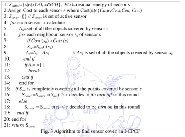
1: Sinitial={s|E(s)>0, sϵSCH}, E(s)=residual energy of sensor s 2:Assign Cost to each sensor s where Cost(s)ϵ{Cmw,Cws,Cea, Ccc) 3: Scover={} // Scover is set of active sensor

4: for each sensor s calculate

5: As=set of all the objects covered by sensor s 6: for each neighbour sensor sk of sensor s

7: if Cost (sk) <Cost (s) 8: Snei=Sneiᴜ(sk)

9: As=As – Ask // Ask is set of all the objects covered by sensor sk 10: end if

11: ifAs= ={} 12: break 13: end if 14: end for

15: if Snei is completelycovering all the points covered by sensor s

16: Scover=Scoverᴜ(Snei) // s decides to be turn off in this round 17: else

18: Scover = Scoverᴜ(s) // s decided to be turn on in this round 19: end if

20: end for 21: return Scover

Fig. 3 Algorithm to find sensor cover in I-CPCP

In Fig. 3, line 1 contains all the remaining sensors after deciding cluster heads in Fig. 2. The respective weighted costs are

assigned to each sensor (line 2). The set of active sensors (sensor cover) is generated through line 4-20. To do so, for each sensor

s, the set of all neighboring sensors with lower weighted cost are selected (line 6-14). If these neighbors’ collectively covering all the objects covered by sensor s (line 15), then sensor s can go to sleep state (line 16), otherwise, it is included in current sensor cover (line -18). Thus, at the end of Algorithm in Fig. 3, a cover set is generated which completely covers all the objects

in the given field.

4.3 Phase III: Routing

This phase describes how the collected data is to be transferred to the base station. The cluster members send their data to

their respective cluster heads which in turn send to the base station. In case, the cluster heads are not able to send the data

directly to base station, then they send via those cluster heads having least associated coverage aware cost with them. In this

phase, the cluster members do not take part in data communication.

5.

Simulation

The main objective of the sensor cover generation is to save the network energy so that the network lifetime can be

prolonged. One of the most commonly used network lifetime is defined [15] as the time of start-up of the network till some

For simulation, we have considered the square area of size 200M*200M in which there are 500 objects placed randomly.

We have evaluated the results by deploying the sensors ranging from 50 to 250 with fix sensing range Rsen=70M. We assume

that the base station is fixed and located outside the network. Sensors are generated in terms of their coordinates which are

generated by Pseudo-random number generation routine. All simulations were performed in MATLAB (R2009) on core i3 with

2.10GHz processor and 4GB RAM system

5.1 Energy Model

In the simulation, we compute the transmission and receiving energy consumption based on the free-space energy model

defined in [20].

The energy required to transmit (Etx) and receive (Erx) a P-bit packet is given below.

Etx=P×(Eamp+εfs×dn) (10)

Erx=P×Eamp (11)

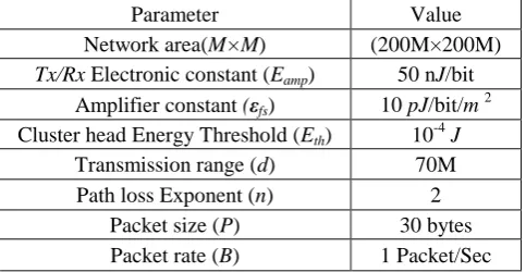
Eamp and εfs are the parameters of the transmission/reception circuitry, and n is the path-loss exponent, listed in Table 1. By

putting all the values specified in Table 1 for simulation in equations (10) and (11), we obtain the transmission and receiving

energy consumed as follows:

Etx=30×8(50×10-9+10×10-12×(702) J

=240(50×10-9+49×10-9)J

=0.24 ×10-4J

(12)

Similarly,

Erx=0.12×10-4J (13)

Therefore, energy consumed by a sensor node to transmit a message of 30 bytes is 0.24 ×10-4 J. In the same way, the total energy consumed by a cluster head to receive the message and to transmit further to the base station is Etx+Erx. By adding

equations (12) and (13), we obtained total energy consumed (14) as follows:

Etx+Erx=0.36×10-4J (14)

Table 1 Parameters and their acronyms used in simulation

Parameter Value

Network area(M× M) (200M×200M) Tx/Rx Electronic constant (Eamp) 50 nJ/bit

Amplifier constant (εfs) 10 pJ/bit/m 2 Cluster head Energy Threshold (Eth) 10-4 J

Transmission range (d) 70M Path loss Exponent (n) 2

5.2 Simulation Results

Here, our objective is to discuss lifetime achieved and execution time taken in our heuristic. We compare the lifetime

achieved and execution time of our heuristic with that of generic CPCP [11] by considering homogenous and heterogeneous

WSNs. We discuss the network lifetime and execution time by considering four different coverage aware costs as discussed in

[11]. These costs include Cmw, Cws, Cea and, Ccc. In homogenous WSNs, we have taken the initial energy of the nodes as

3*10-4J. Here, the network lifetime and the execution time of our heuristic and CPCP [11] with respect to all costs, i.e., (Cmw, Cws, Cea and Ccc) have been computed as shown in Fig. 4 to Fig. 7 respectively.

As evident from these Fig. 4 to Fig. 7, our heuristic provides better networks lifetime as compared to CPCP for all the costs.

As the number of sensor grows, the gap in lifetime achieved by CPCP and our heuristic increases because, due to increase in

number of sensors, connectivity between neighbour sensors is also increases. Therefore, our heuristic selects less number of

sensors for coverage phase which result in increased total network lifetime.

Fig. 4 Network lifetime (homogenous WSNs) achieved by proposed I-CPCP and CPCP [11] with cost Cmw

Fig. 5 Network lifetime (homogenous WSNs) achieved by proposed I-CPCP and CPCP [11] with cost Cws

Fig. 6Network lifetime (homogenous WSNs) achieved by proposed I-CPCP and CPCP [11] with cost Cea

Fig. 7Network lifetime (homogenous WSNs) achievedby proposed I-CPCP and CPCP [11] with cost Ccc

In proposed heuristic I-CPCP, we perform minimalization process to reduce number of sensors in sensor cover that in turn

reduces the energy usages. The minimalization process needs some time for its execution, however, the total execution time

Table 2 Execution time taken (in seconds) by proposed heuristic (I-CPCP) and CPCP [11] in homogenous WSNs

Sensor Cmw Cws Ccc Cea

CPCP I-CPCP CPCP I-CPCP CPCP I-CPCP CPCP I-CPCP

50 0.11 0.15 0.28 0.28 4.25 4.45 0.26 0.33

100 0.14 0.18 0.42 0.55 9.11 9.65 0.51 0.92

150 0.21 0.32 0.63 0.92 13.95 16.2 0.67 1.35 200 0.35 0.49 0.9 1.46 20.13 23.53 0.81 1.62 250 0.45 0.61 1.16 2.07 26.39 36.51 1.1 2.15

In case of heterogeneous network, we have allocated initial energy to sensors by generating randomly in the range 1*10-4J to 5*10-4J. As shown in Fig. 8 to Fig. 11, in this case also our heuristic (I-CPCP) has much better network life time as compared to that of CPCP [11] for all the four coverage aware costs. Again, increasing the number of nodes, it behaves similar to

homogenous network.

Fig. 8Network lifetime (heterogeneous WSNs) achievedby proposed I-CPCP and CPCP [11] with cost Cmw

Fig. 9Network lifetime (heterogeneous WSNs) achievedby proposed I-CPCP and CPCP [11] with cost Cws.

Fig. 10Network lifetime (heterogeneous WSNs) achievedby proposed I-CPCP and CPCP [11] with cost Cea.

Fig. 11Network lifetime (heterogeneous WSNs) achievedby proposed I-CPCP and CPCP [11] with cost Ccc.

The behaviour of execution time in this case is quite similar as that of the homogenous network as shown in Table 3. Thus,

our heuristic provide much longer network lifetime without requiring much overhead in execution time. We may conclude that

our heuristic has better performance as compared toRef. [11].

Sensor Cmw Cws Ccc Cea CPCP I-CPCP CPCP I-CPCP CPCP I-CPCP CPCP I-CPCP 50 0.10 0.13 0.18 0.22 3.43 3.46 0.2 0.29 100 0.14 0.17 0.42 0.56 7.79 8.46 0.46 0.82 150 0.21 0.28 0.61 0.89 13.4 15.87 0.66 1.38 200 0.32 0.39 0.86 1.25 19.66 24.08 0.91 1.78 250 0.45 0.61 1.17 1.76 24.78 31.71 1.12 2.52

6.

Conclusions

In this paper, we have discussed an improved coverage preservation clustering protocol (I-CPCP)) in clustered wireless

sensor networks. We explore various weighted coverage costs in order to select cluster head and to form sensor covers to

monitor the given region for longest possible period. In the proposed protocol, we jointly consider residual energy as well as

coverage redundancy of sensors to generate sensor cover and cluster heads which results in improved network lifetime as

compared to those approaches [2, 3, 4, and 5] which only consider either at a time. Further, we minimalize the generated sensor

covers so that only minimum numbers of sensors are used in each sensor cover. Due to this minimalization process, our

proposed protocol (I-CPCP) outperforms generic CPCP [11] in terms of lifetime achieved in homogeneous as well as in

heterogeneous network. In our future work, we may extend this improved protocol for target connected coverage problem,

target Q-coverage problem and target coverage with multiple sensing ranges. We will also implement I-CPCP and CPCP

protocol on specific sensor test- bed with respect to all coverage aware costs discussed in this paper.

References

[1] I. F. Akyildiz, W. Su, Y. Sankarasubramaniam, and E. Cayirci, “A survey on sensor networks,” IEEE Communications Magazine, vol. 40, no. 8, pp.102-114, 2002.

[2] M. Cardei andD. Z. Du, “Improving wireless sensor network lifetime through power aware organization,” ACM Wireless Networks, vol. 11, pp. 333–340, 2005.

[3] M. Cardei, M. T. Thai, Y. Li, and W. Wu, “Energy-efficient target coverage in wireless sensor networks,” Proc. IEEE Infocom, IEEE press, March. 2005, pp. 1976-1984.

[4] S. Mini, S. K. Udgata, and S. L. Sabat, “Sensor deployment and scheduling for target coverage problem in wireless sensor networks,” IEEE SENSORS Journal, vol. 14, no. 3, pp. 636-644, 2014.

[5] Manju and A. K Pujari, “High-Energy-First (HEF) heuristic for energy efficient target coverage problem,” International Journal of Adhoc sensor and Ubiquitous Computing, vol. 2, no. 1, March 2011.

[6] A. Panconesi and M. Sozio, “Fast distributed scheduling via primal-dual,” Proc. the twentieth annual symposium on Parallelism in algorithms and architectures, 2008, pp. 229-235.

[7] V. Kumar, S. Jain, and S. Tiwari, “Energy efficient clustering algorithms in wireless sensor networks, A survey,” IJCSI International Journal of Computer Science Issues, vol. 8 , no. 2, pp. 259-268, October 2011.

[8] M. Chatterjee, S. Das, and D. Turgut, “WCA: A weighted clustering algorithm for mobile ad hoc networks,” Journal of Cluster Computing, Special issue on Mobile Ad hoc Networking ,vol. 5, no. 2, pp. 193-204, April 2002.

[9] S. Yi, J. Heo, and Y. Cho, “PEACH: power-efficient and adaptive clustering hierarchy protocol for wireless sensor networks,” Computer Communications, vol. 30, no. 14, pp. 2842-2852, 2007.

[10] Z. Liu, Q. Zheng, L. Xue, and X. Guan, “A distributed energy-efficient clustering algorithm with improved coverage in wireless sensor networks,” Future Generation Computer System, vol. 28, no. 5, pp. 780-790, May 2012.

[11] S. Soro and W. B. Heinzelman, “Cluster head election technique for coverage preservation in wireless sensor networks,” Ad Hoc Networks, vol. 7, no. 5, pp. 955-972, July 2009.

[12] W. B. Heinzelman, A. P. Chandrakasan, and H. Balakrishnan, “An application-specific protocol architecture for wireless

microsensor networks,” IEEE Transactions on Wireless Communications, vol. 1, no. 4, pp. 660−670, 2002.

[14] O. Younis and S. Fahmy, “HEED: A hybrid, energy-efficient, distributed clustering approach for ad hoc sensor networks,”

IEEE Transactions on Mobile Computing, vol. 3, no. 4, pp. 660-669, 2004.

[15] S. Gamwarige and C. Kulasekere, “An algorithm for energy driven cluster head rotation in a distributed wireless sensor network,” Proc. the International Conference on Information and Automation, pp. 354-359, 2005.

[16] M. Qin and R. Zimmermm, “An energy-efficient voting-based clustering algorithm for sensor networks,” Proc. Software

Engineering, Artificial Intelligence, Networking and Parallel/Distributed Computing, IEEE Press, May. 2005, pp. 444-451.

[17] G. Smaragdakis, I. Matta, and A. Bestavros, “SEP: a stable election protocol for clustered heterogeneous wireless sensor networks,” Proc. the 2nd International Workshops on Sensor and Actor Network Protocols and Applications. Boston, USA, IEEE Press, 2004, pp. 223-233.

[18] D. Kumar, T. C. Aseri, and R. B. Patel, “EEHC: energy efficient heterogeneous clustered scheme for wireless sensor networks,” Computer Communications, vol. 32, no. 4, pp. 662-667, March 2009.

[19] H. Zhen, Y. Li, and G. J. Zhang, “Efficient and dynamic clustering scheme for heterogeneous multi-level wireless sensor

networks,” Acta Automatica Sinica, vol. 39, no. 4, April 2013.

[20] W. B. Heinzelman, A. P. Chandrakasan, and H. Balakrishnan, “An application specific protocol architecture for wireless microsensor networks,” IEEE Transactions on Wireless Communications, vol. 1, no. 4, 2002.

[21] M. Chaudhary and A. K. Pujari, “Q-coverage problem in wireless sensor networks,” Proc. Int. Conf. Distrib. Comput.

Networks, Springer Berlin Heidelberg press, 2009, pp. 325–330.

[22] D. Bajaj and Manju, “Maximum Coverage Heuristic (MCH) for target coverage problem in WSN,” Proc. IACC, IEEE press, Feb. 2014, pp. 300-305.

[23] S. Venkatesh and K. M. Mehata, “A competent fault tolerant system using simulated annealing approach for target tracking

in wireless sensor networks,” Proc. Computer Communication and Informatics (ICCCI), 2014 International Conference on, IEEE press, Jan. 2014, pp.1-6.

[24] J. Kim, H. W. Lee, and S. Chong, “TAES: Traffic-aware energy-saving base station sleeping and clustering in cooperative networks,” Proc. Modeling and Optimization in Mobile, Ad Hoc, and Wireless Networks (WiOpt), 2015, 13th

International Symp, IEEE press, May. 2015, pp.259-266.

[25] S. H. Seo, J. Won, S. Sultana, and E. Bertino, “Effective key management in dynamic wireless sensor networks,” in Information Forensics and Security, IEEE Transactions on, vol. 10, no. 2, pp.371-383, 2015.

[26] M. Collotta and G. Pau, “A novel energy management approach for smart homes using Bluetooth low energy,” IEEE

Journal on Selected Areas in Communications, vol. 33, no. 12, pp.2988-2996, 2015.

[27] Y. C. Lee, H. Y. Lai, and P. J. Lee, “Cryptanalysis and improvement of the robust user authentication scheme for wireless sensor networks,” International Journal of Engineering and Technology Innovation, vol. 2, no. 4, pp. 283-292, 2012. [28] F. Carrabs, R. Cerulli, C. D'Ambrosio, and A. Raiconi, “A hybrid exact approach for maximizing lifetime in sensor

networks with complete and partial coverage constraints,” Journal of Network and Computer Applications, vol. 58, pp.

12-22, 2015.