A Comparison of Optimization Methods and Software for Large-scale
L1-regularized Linear Classification
Guo-Xun Yuan [email protected]
Kai-Wei Chang [email protected]
Cho-Jui Hsieh [email protected]
Chih-Jen Lin [email protected]
Department of Computer Science National Taiwan University Taipei 106, Taiwan
Editor: Sathiya Keerthi
Abstract
Large-scale linear classification is widely used in many areas. The L1-regularized form can be applied for feature selection; however, its non-differentiability causes more difficulties in training. Although various optimization methods have been proposed in recent years, these have not yet been compared suitably. In this paper, we first broadly review existing methods. Then, we discuss state-of-the-art software packages in detail and propose two efficient implementations. Extensive comparisons indicate that carefully implemented coordinate descent methods are very suitable for training large document data.
Keywords: L1 regularization, linear classification, optimization methods, logistic regression,
support vector machines, document classification
1. Introduction
Recently, L1-regularized classifiers have attracted considerable attention because they can be used to obtain a sparse model. Given a set of instance-label pairs (xi,yi), i=1, . . . ,l, xi ∈Rn, yi ∈
{−1,+1}, training an L1-regularized linear classifier involves the following unconstrained opti-mization problem:
min
w f(w)≡ kwk1+C
l
∑
i=1
ξ(w; xi,yi), (1)
wherek · k1denotes the 1-norm andξ(w; xi,yi)is a non-negative (convex) loss function. The
regu-larization termkwk1is used to avoid overfitting the training data. The user-defined parameter C>0 is used to balance the regularization and loss terms.
of its loss function. This drawback leads to greater difficulty in solving the optimization problem. Therefore, certain considerations are required to handle the non-differentiability.
Many loss functions can be used for linear classification. A commonly used one is logistic loss:
ξlog(w; x,y) =log(1+e−yw Tx
). (2)
This loss function is twice differentiable. Note that minimizing logistic loss is equivalent to maxi-mizing the likelihood, whereas minimaxi-mizing the regularized loss in (1) is equivalent to maximaxi-mizing the posterior with independent Laplace priors on the parameters. Two other frequently used func-tions are the L1- and the L2-loss funcfunc-tions:
ξL1(w; x,y) =max(1−ywTx,0) and (3) ξL2(w; x,y) =max(1−ywTx,0)2. (4) Because of the max(·)operation, the L1-loss function is not differentiable. On the other hand, L2 loss is differentiable, but not twice differentiable (Mangasarian, 2002). We refer to (1) with logistic loss as L1-regularized logistic regression and (1) with L1/L2 loss as L1-regularized L1-/L2-loss support vector machines (SVMs).
In some applications, we require a bias term b (also called as an intercept) in the loss function; therefore, wTx in (2)–(4) is replaced with wTx+b. For example, the logistic loss function becomes
ξlog(w,b; x,y) =log
1+e−y(wTx+b)
.
The optimization problem then involves variables w and b:
min
w,b kwk1+C l
∑
i=1
ξ(w,b; xi,yi). (5)
Because b does not appear in the regularization term, most optimization methods used to solve (1) can solve (5) as well. In this paper, except whenever b is required, we mainly consider the formulation (1).
1.1 Basic Properties of (1)
In this paper, we assume that the loss functionξ(w; xi,yi)is convex, differentiable, and nonnegative.
The proof presented in Appendix A shows that (1) attains at least one global optimum. Unlike L2 regularization, which leads to a unique optimal solution, here, (1) may possess multiple optimal solutions. We use w∗to denote any optimal solution of (1). The convexity of f(w)implies that all optimal solutions have the same function value, which is denoted as f∗. For more information about the set of optimal solutions, see, for example, Hale et al. (2008, Section 2).
From standard convex analysis, w∗ is optimal for (1) if and only if w∗ satisfies the following optimality conditions:
∇jL(w∗) +1=0 if w∗j>0,
∇jL(w∗)−1=0 if w∗j<0,
−1≤∇jL(w∗)≤1 if w∗j=0,
(6)
where L(w)is the loss term in (1):
L(w)≡C l
∑
i=1
ξ(w; xi,yi). (7)
1.2 Organization and Notation
The remainder of this paper is organized as follows. In Section 2, we briefly survey existing ap-proaches. Section 3 lists state-of-the-art L1-regularized logistic regression packages compared in this study. Sections 4–6 discuss these packages in detail; two of these (Sections 4.1.2 and 5.1) are our proposed implementations. In Section 7, we extend several methods to train L2-loss SVMs. Section 8 describes the extensive experiments that were carried out. Comparison results indicate that decomposition methods (Section 4) are very suitable for large-scale document data. Finally, the discussions and conclusions are presented in Section 9. A supplementary file including additional details and descriptions of experiments is available athttp://www.csie.ntu.edu.tw/˜cjlin/ papers/l1/supplement.pdf
In this study, we use consistent notation to describe several state-of-the-art methods that are considered. The following table lists some frequently used symbols:
l: number of instances n: number of features
i: index for a data instance j: index for a data feature
k: iteration index for an optimization algorithm
We may represent training instances(xi,yi),i=1, . . . ,l in the following form:
X=
xT1
.. .
xTl
∈Rl×n and y=
y1 .. . yl
∈ {−1,+1}l.
For any vector v, we consider the following two representations for sub-vectors:
vt:s≡[vt, . . . ,vs]T and vI≡[vi1, . . . ,vi|I|]
where I={i1, . . . ,i|I|}is an index set. Similarly,
XI,:≡
xTi1
.. .
xTi|
I|
. (8)
The functionτ(s)gives the first derivative of the logistic loss function log(1+es):
τ(s)≡ 1
1+e−s. (9)
An indicator vector for the jth component is
ej≡[0, . . . ,0 | {z }
j−1
,1,0, . . . ,0]T. (10)
We usek · kork · k2to denote the 2-norm andk · k1to denote the 1-norm.
2. A Survey of Existing Methods
In this section, we survey existing methods for L1-regularized problems. In Sections 2.1–2.3, we focus on logistic regression and L2-loss SVMs for data classification. Section 2.5 briefly discusses works on regression problems using the least-square loss.
2.1 Decomposition Methods
Decomposition methods are a classical optimization approach. Because it is difficult to update all variables simultaneously, at each iteration, we can choose a subset of variables as the working set and fix all others. The resulting sub-problem contains fewer variables and is easier to solve. The various decomposition methods that have been applied to solve L1-regularized problems are categorized into two types according to the selection of the working set.
2.1.1 CYCLICCOORDINATEDESCENTMETHODS
A simple coordinate descent method cyclically chooses one variable at a time and solves the fol-lowing one-variable sub-problem:
min
z gj(z)≡ f(w+zej)−f(w), (11)
where ej is defined in (10). This function gj(z)has only one non-differentiable point at z=−wj.
In optimization, the cyclic method for choosing working variables is often called the Gauss-Seidel rule (Tseng and Yun, 2007).
Several works have applied coordinate descent methods to solve (1) with logistic loss. Here, a difficulty arises in that sub-problem (11) does not have a closed-form solution. Goodman (2004) assumed nonnegative feature values (i.e., xi j ≥0,∀i,j) and then approximated gj(z)by a function Aj(z)at each iteration. Aj(z)satisfies Aj(z)≥gj(z),∀z, and Aj(0) =gj(0) =0; therefore,
approach can be extended to solve the original L1-regularized logistic regression by taking the sign of wj into consideration.
Genkin et al. (2007) implemented a cyclic coordinate descent method calledBBRto solve L1-regularized logistic regression. BBR approximately minimizes sub-problem (11) in a trust region and applies one-dimensional Newton steps. Balakrishnan and Madigan (2005) reported an extension ofBBRfor online settings.
In Section 4.1.2, we propose a coordinate descent method by extending Chang et al.’s (2008) approach for L2-regularized classifiers. Chang et al. (2008) approximately solved the sub-problem (11) by a one-dimensional Newton direction with line search. Experiments show that their approach outperforms aBBRvariant for L2-regularized classification. Therefore, for L1 regularization, this approach might be faster thanBBR. Hereafter, we refer to this efficient coordinate descent method asCDN(coordinate descent using one-dimensional Newton steps).
Tseng and Yun (2007) broadly discussed decomposition methods for L1-regularized problems. One of their approaches is a cyclic coordinate descent method. They considered a general cyclic setting so that several working variables are updated at each iteration. We show thatCDNis a special case of their general algorithms.
If we randomly select the working variable, then the procedure becomes a stochastic coordinate descent method. Shalev-Shwartz and Tewari (2009, Algorithm 2) recently studied this issue. Duchi and Singer (2009) proposed a similar coordinate descent method for the maximum entropy model, which is a generalization of logistic regression.
2.1.2 VARIABLESELECTIONUSINGGRADIENTINFORMATION
Instead of cyclically updating one variable, we can choose working variables based on the gradient information.1 This method for selecting variables is often referred to as the Gauss-Southwell rule (Tseng and Yun, 2007). Because of the use of gradient information, the number of iterations is fewer than those in cyclic coordinate descent methods. However, the cost per iteration is higher. Shevade and Keerthi (2003) proposed an early decomposition method with the Gauss-Southwell rule to solve (1). In their method, one variable is chosen at a time and one-dimensional Newton steps are applied; therefore, their method differs from the cyclic coordinate descent methods described in Section 2.1.1 mainly in terms of finding the working variables. Hsieh et al. (2008) showed that for L2-regularized linear classification, maintaining the gradient for selecting only one variable at a time is not cost-effective. Thus, for decomposition methods using the gradient information, a larger working set should be used at each iteration.
In the framework of decomposition methods proposed by Tseng and Yun (2007), one type of method selects a set of working variables based on the gradient information. The working set can be large, and therefore, they approximately solved the sub-problem. For the same method, Yun and Toh (2009) enhanced the theoretical results and carried out experiments with document classification data. We refer to their method asCGD-GSbecause the method described in Tseng and Yun (2007) is called “coordinate gradient descent” and a Gauss-Southwell rule is used.
2.1.3 ACTIVESETMETHODS
Active set methods are a popular optimization approach for linear-constrained problems. For prob-lem (1), an active method becomes a special decomposition method because at each iteration, a
sub-problem over a working set of variables is solved. The main difference from decomposition methods described earlier is that the working set contains all non-zero variables. Therefore, an ac-tive set method iteraac-tively predicts what a correct split of zero and non-zero elements in w is. If the split is correct, then solving the sub-problem gives the optimal values of non-zero elements.
Perkins et al. (2003) proposed an active set method for (1) with logistic loss. This implementa-tion uses gradient informaimplementa-tion to predict w’s zero and non-zero elements.
2.2 Methods by Solving Constrained Optimization Problems
This type of method transforms (1) to equivalent constrained optimization problems. We further classify them into two groups.
2.2.1 OPTIMIZATIONPROBLEMS WITHSMOOTHCONSTRAINTS
We can replace w in (1) with w+−w−, where w+ and w− are both nonnegative vectors. Then, problem (1) becomes equivalent to the following bound-constrained optimization problem:
min w+,w−
n
∑
j=1 w+j +
n
∑
j=1 w−j +C
l
∑
i=1
ξ(w+−w−; xi,yi)
subject to w+j ≥0,w−j ≥0, j=1, . . . ,n.
(12)
The objective function and constraints of (12) are smooth, and therefore, the problem can be solved by standard bound-constrained optimization techniques. Schmidt et al. (2009) proposed Projec-tionL1to solve (12). This is an extension of the “two-metric projection” method (Gafni and Bert-sekas, 1984). Limited-memory quasi Newton implementations, for example, LBFGS-B by Byrd et al. (1995) andBLMVM by Benson and Mor´e (2001), require function/gradient evaluations and use a limited amount of memory to approximate the Hessian matrix. Kazama and Tsujii (2003) pre-sented an example of usingBLMVMfor (12). Lin and Mor´e’s (1999) trust region Newton method (TRON) can also be applied to solve (12). In addition to function/gradient evaluations,TRONneeds to calculate Hessian-vector products for faster convergence. Lin et al. (2008) appliedTRONto solve L2-regularized logistic regression and showed thatTRONoutperformsLBFGSfor document data. No previous work has appliedTRONto solve L1-regularized problems, and therefore, we describe this in Section 5.1.
Koh et al. (2007) proposed an interior point method to solve L1-regularized logistic regression. They transformed (1) to the following constrained problem:
min w,u
n
∑
j=1 uj+C
l
∑
i=1
ξ(w; xi,yi)
subject to −uj≤wj≤uj, j=1, . . . ,n.
(13)
Equation (13) can be made equivalent to (12) by setting
w+j =uj+wj
2 and w
− j =
uj−wj
2 .
2.2.2 OPTIMIZATIONPROBLEMS WITHNON-SMOOTHCONSTRAINTS
It is well-known that for any choice of C in (1), there exists a corresponding K such that (1) is equivalent to the following problem:
min w
l
∑
i=1
ξ(w; xi,yi)
subject to kwk1≤K.
(14)
See the explanation in, for example, Donoho and Tsaig (2008, Section 1.2). Notice that in (14), the constraint is not smooth at{w|wj =0 for some j}. However, (14) contains fewer variables and
constraints than (12). Lee et al. (2006) applied the LARS algorithm described in Efron et al. (2004) to find a Newton direction at each step and then used a backtracking line search to minimize the objective value. Kivinen and Warmuth’s (1997) concept of exponentiated gradient (EG) can solve (14) with additional constraints wj≥0, ∀j. In a manner similar to the technique for constructing
(12), we can remove the nonnegative constraints by replacing w with w+−w−. If k is the iteration index,EGupdates w by the following rule:
wkj+1=w
k
jexp −ηk∇j ∑li=1ξ(wk; xi,yi)
Zk
,
where Zkis a normalization term for maintainingkwkk1=K, ∀k andηk is a user-defined learning
rate. Duchi et al. (2008) applied a gradient projection method to solve (14). The update rule is
wk+1=arg min w
n
k wk−ηk∇
∑
l i=1ξ(w
k; x i,yi)
−wk
kwk1≤K
o
. (15)
They developed a fast algorithm to project a solution to the closest point satisfying the constraint. They also considered replacing the gradient in (15) with a stochastic sub-gradient. In a manner sim-ilar to (15), Liu et al. (2009) proposed a gradient projection method calledLassploreand carefully addressed the selection of the learning rateηk. However, they evaluated their method only on data
with no more than 2,000 instances.2
Kim and Kim (2004) discussed a coordinate descent method to solve (14). They used the gradi-ent information to select an elemgradi-ent wj for update. However, because of the constraintkwk1≤K, the whole vector w is normalized at each step. Thus, the setting is very different from the un-constrained situations described in Section 2.1.1. Kim et al. (2008) made further improvements to realize faster convergence.
Active set methods have also been applied to solve (14). However, in contrast to the active set methods described in Section 2.1.3, here, the sub-problem at each iteration is a constrained optimization problem. Roth (2004) studied general loss functions including logistic loss.
2.3 Other Methods for L1-regularized Logistic Regression/L2-loss SVMs
We briefly review other methods in this section.
2.3.1 EXPECTATIONMAXIMIZATION
Many studies have considered Expectation Maximization (EM) frameworks to solve (1) with logis-tic loss (e.g., Figueiredo, 2003; Krishnapuram et al., 2004, 2005). These works find an upper-bound function ˆf(w)≥ f(w),∀w, and perform Newton steps to minimize ˆf(w). However, as pointed out by Schmidt et al. (2009, Section 3.2), the upper-bound function ˆf(w)may not be well-defined at some wi=0 and hence certain difficulties must be addressed.
2.3.2 STOCHASTICGRADIENTDESCENT
Stochastic gradient descent methods have been successfully applied to solve (1). At each iteration, the solution is updated using a randomly selected instance. These types of methods are known to efficiently generate a reasonable model, although they suffer from slow local convergence. Under an online setting, Langford et al. (2009) solved L1-regularized problems by a stochastic gradient descent method. Shalev-Shwartz and Tewari (2009) combined Langford et al.’s (2009) method with other techniques to obtain a new stochastic gradient descent method for (1).
2.3.3 QUASINEWTONMETHODS
Andrew and Gao (2007) proposed an Orthant-Wise Limited-memory quasi Newton (OWL-QN) method. This method is extended fromLBFGS(Liu and Nocedal, 1989), a limited memory quasi Newton approach for unconstrained smooth optimization. At each iteration, this method finds a sub-space without considering some dimensions with wj =0 and obtains a search direction
simi-lar toLBFGS. A constrained line search on the same sub-space is then conducted and the property wkj+1wkj≥0 is maintained. Yu et al. (2010) proposed a quasi Newton approach to solve non-smooth convex optimization problems. Their method can be used to improve the line search procedure in
OWL-QN.
2.3.4 HYBRIDMETHODS
Shi et al. (2010) proposed a hybrid algorithm for (1) with logistic loss. They used a fixed-point method to identify the set{j|w∗j=0}, where w∗is an optimal solution, and then applied an interior
point method to achieve fast local convergence.
2.3.5 QUADRATICAPPROXIMATIONFOLLOWEDBYCOORDINATEDESCENT
Krishnapuram et al. (2005) and Friedman et al. (2010) replaced the loss term with a second-order approximation at the beginning of each iteration and then applied a cyclic coordinate descent method to minimize the quadratic function. We will show that an implementation in Friedman et al. (2010) is efficient.
2.3.6 CUTTINGPLANEMETHODS
2.3.7 APPROXIMATINGL1 REGULARIZATION BYL2 REGULARIZATION
Kujala et al. (2009) proposed the approximation of L1-regularized SVMs by iteratively reweighting training data and solving L2-regularized SVMs. That is, using the current wj, they adjusted the jth
feature of the training data and then trained an L2-regularized SVM in the next step.
2.3.8 SOLUTIONPATH
Several works have attempted to find the “solution path” of (1). The optimal solution of (1) varies according to parameter C. It is occasionally useful to find all solutions as a function of C; see, for example, Rosset (2005), Zhao and Yu (2007), Park and Hastie (2007), and Keerthi and Shevade (2007). We do not provide details of these works because this paper focuses on the case in which a single C is used.
2.4 Strengths and Weaknesses of Existing Methods
Although this paper will compare state-of-the-art software, we discuss some known strengths and weaknesses of existing methods.
2.4.1 CONVERGENCESPEED
Optimization methods using higher-order information (e.g., quasi Newton or Newton methods) usu-ally enjoy fast local convergence. However, they involve an expensive iteration. For example, New-ton methods such asTRONorIPMneed to solve a large linear system related to the Hessian matrix. In contrast, methods using or partially using the gradient information (e.g., stochastic gradient de-scent) have slow local convergence although they can more quickly decrease the function value in the early stage.
2.4.2 IMPLEMENTATIONEFFORTS
Methods using higher-order information are usually more complicated. Newton methods need to include a solver for linear systems. In contrast, methods such as coordinate descent or stochas-tic gradient descent methods are easy to implement. They involve only vector operations. Other methods such as expectation maximization are intermediate in this respect.
2.4.3 HANDLINGLARGE-SCALEDATA
In some methods, the Newton step requires solving a linear system of n variables. Inverting an n×n matrix is difficult for large n. Thus, one should not use direct methods (e.g., Gaussian elimination) to solve the linear system. Instead,TRONandIPMemploy conjugate gradient methods and Friedman et al. (2007) use coordinate descent methods. We observe that for existing EM implementations, many consider direct inversions, and therefore, they cannot handle large-scale data.
2.4.4 FEATURECORRELATION
2.4.5 DATATYPE
No method is the most suitable for all data types. A method that is efficient for one application may be slow for another. This paper is focused on document classification, and a viable method must be able to easily handle large and sparse features.
2.5 Least-square Regression for Signal Processing and Image Applications
Recently, L1-regularized problems have attracted considerable attention for signal processing and image applications. However, they differ from (1) in several aspects. First, yi∈R, and therefore, a
regression instead of a classification problem is considered. Second, the least-square loss function is used:
ξ(w; xi,yi) = (yi−wTxi)2. (16)
Third, in many situations, xiare not directly available. Instead, the product between the data matrix X and a vector can be efficiently obtained through certain operators. We briefly review some of the many optimization methods for least-square regression. If we use formulation (14) with non-smooth constraints, the problem reduces to LASSO proposed by Tibshirani (1996) and some early optimization studies include, for example, Fu (1998) and Osborne et al. (2000a,b). Fu (1998) ap-plied a cyclic coordinate descent method. For least-square loss, the minimization of the one-variable sub-problem (11) has a closed-form solution. Sardy et al. (2000) also considered coordinate descent methods, although they allowed a block of variables at each iteration. Wu and Lange (2008) con-sidered a coordinate descent method, but used the gradient information for selecting the working variable at each iteration. Osborne et al. (2000a) reported one of the earliest active set methods for L1-regularized problems. Roth’s (2004) method for general losses (see Section 2.2.2) reduces to this method if the least-square loss is used. Friedman et al. (2007) extended Fu’s coordinate de-scent method to find a solution path. Donoho and Tsaig (2008) also obtained a solution path. Their procedure requires solving a linear system of a matrix X:T,JX:,J, where J is a subset of {1, . . . ,n}.
Figueiredo et al. (2007) transformed the regression problem to a bound-constrained formula in (12) and applied a projected gradient method. Wright et al. (2009) proposed the iterative minimization of the sum of the L1 regularization term and a quadratic approximation of the loss term. In the quadratic approximation, they used a diagonal matrix instead of the Hessian of the loss term, and therefore, the minimization can be easily carried out. Hale et al. (2008) proposed a fixed point method to solve (1) with the least-square loss (16). Their update rule is generated from a fixed-point view; however, it is very similar to a gradient projection algorithm.
The dual of LASSO and the dual of (1) have been discussed in Osborne et al. (2000b) and Kim et al. (2007), respectively. However, thus far, there have been few optimization methods for the dual problem. Tomioka and Sugiyama (2009) proposed a dual augmented Lagrangian method for L1-regularized least-square regression that theoretically converges super-linearly.
of applications. The interior point method for logistic regression by solving (13) has been applied to the least-square regression problem (Kim et al., 2007). Duchi et al. (2008) compared their gradient projection implementation (see Section 2.2.2) with interior point methods using both logistic and least-square losses. In Section 2.1.2, we mentioned a decomposition methodCGD-GSby Yun and Toh (2009). In the same paper, Yun and Toh have also investigated the performance ofCGD-GSon regression problems.
In this paper, we focus on data classification, and therefore, our conclusions may not apply to regression applications. In particular, the efficient calculation between X and a vector in some signal processing applications may afford advantages to some optimization methods.
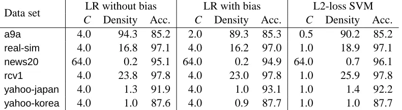
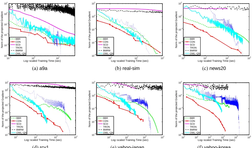
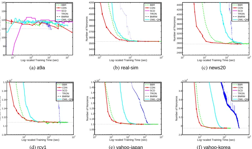
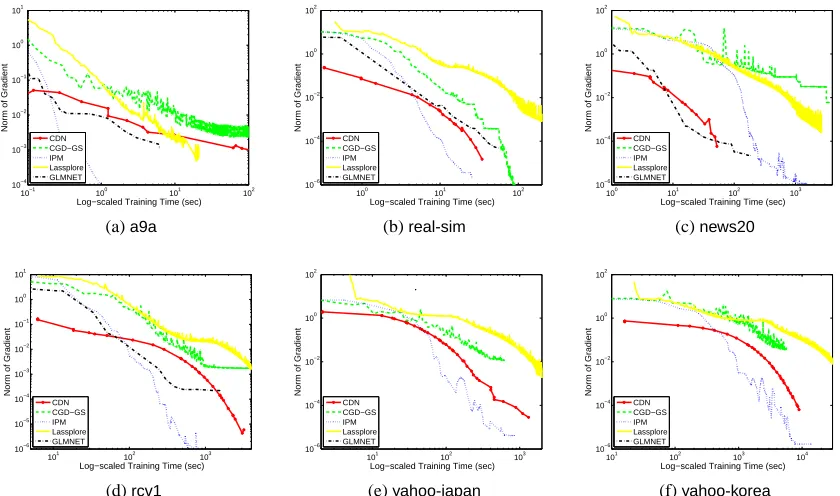
3. Methods and Software Included for Comparison
In the rest of this paper, we compare some state-of-the-art software BBR, SCD, CGD-GS, IPM,
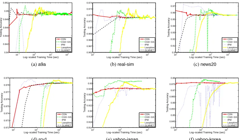
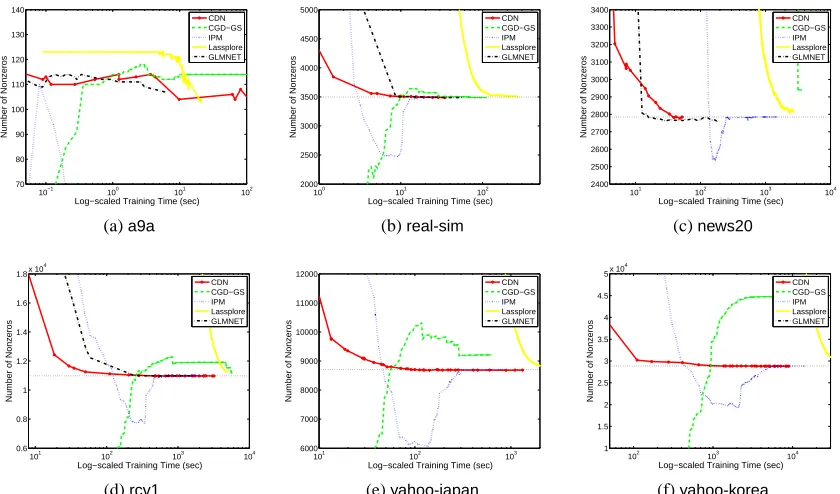
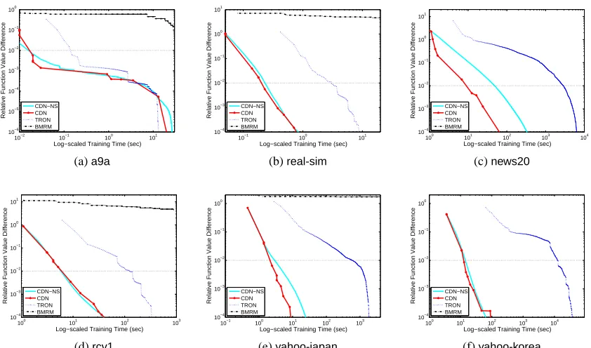
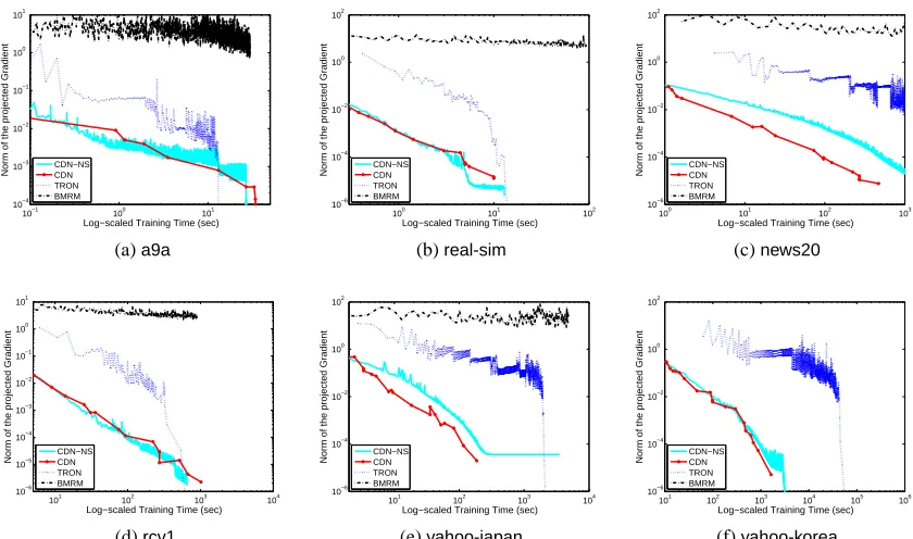
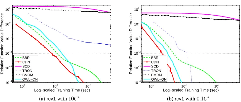
BMRM,OWL-QN,LassploreandGLMNET. We further develop two efficient implementations. One is a coordinate descent method (CDN) and the other is a trust region Newton method (TRON). These packages are selected because of two reasons. First, they are publicly available. Second, they are able to handle large and sparse data sets. We categorize these packages into three groups:
• decomposition methods,
• methods by solving constrained optimization problems,
• other methods,
and describe their algorithms in Sections 4–6. The comparison results are described in Sections 8. Note that classification (logistic regression and L2-loss SVMs) is our focus, and therefore, software for regression problems using the least-square loss (16) is not considered.
4. Decomposition Methods
This section discusses three methods sequentially or randomly choosing variables for update, and one method using gradient information for the working set selection.
4.1 Cyclic Coordinate Descent Methods
From the current solution wk, a coordinate descent method updates one variable at a time to generate
wk,j∈Rn, j=1, . . . ,n+1, such that wk,1=wk, wk,n+1=wk+1, and
wk,j=hwk1+1, . . . ,wkj−+11,wkj, . . . ,wkniT for j=2, . . . ,n.
To update wk,j to wk,j+1, the following one-variable optimization problem is solved: min
z gj(z) =|w k,j
j +z| − |w k,j
j |+Lj(z; wk,j)−Lj(0; wk,j), (17)
where
Algorithm 1 A framework of coordinate descent methods
1. Given w1.
2. For k=1,2,3, . . .(outer iterations) (a) wk,1=wk.
(b) For j=1,2, . . . ,n (inner iterations)
• Find d by solving the sub-problem (17) exactly or approximately. • wk,j+1=wk,j+dej.
(c) wk+1=wk,n+1.
For simplicity, hereafter, we use Lj(z) in most places. If the solution of (17) is d, then we update
the jth element by
wkj,j+1=wkj,j+d.
Typically, a coordinate descent method sequentially goes through all variables and then repeats the same process; see the framework in Algorithm 1. We refer to the process of updating every n elements (i.e., from wkto wk+1) as an outer iteration and the step of updating one element (i.e., from
wk,j to wk,j+1) as an inner iteration. Practically, we only approximately solve (17), where several approaches are discussed below.
Using the same way to obtain the optimality condition in (6), for the one-variable function gj(z),
we have that z=0 is optimal for (17) if and only if
L′j(0) +1=0 if wkj,j>0, L′j(0)−1=0 if wkj,j<0, −1≤L′j(0)≤1 if wkj,j=0.
(18)
The optimality condition at z=0 shows if modifying wkj,jmay decrease the function value or not.
4.1.1 BBR
Genkin et al. (2007) propose a coordinate descent methodBBR for (1) and (5) with logistic loss. This method is extended from Zhang and Oles (2001) for L2-regularized logistic regression. At each inner iteration,BBRapproximately solves the sub-problem (17) by a trust region Newton method. With the trust region∆j, it requires the step z to satisfy
|z| ≤∆j and wkj,j+z (
≥0 if wkj,j>0,
≤0 if wkj,j<0. (19)
The first constraint confines the step size to be in the trust region and∆j is updated at the end of
each inner iteration. Due to the non-differentiable point at z=−wkj,j, the second constraint ensures that the function is differentiable in the search space.
To approximately solve (17),BBRminimizes a quadratic function upper-bounding the function gj(z)in the trust region. Though gj(z)is not differentiable, by considering both cases of wkj,j>0
and wkj,j<0, we obtain the following form:
gj(z) =gj(0) +g′j(0)z+
1 2g
′′
where 0<η<1,
g′j(0)≡
(
L′j(0) +1 if wkj,j>0,
L′j(0)−1 if wkj,j<0, and g ′′
j(ηz)≡L′′j(ηz). (21)
Notice that when wkj,j=0, gj(z)is non-differentiable at z=0 and g′j(0)is not well-defined. We will
discuss this situation later.BBRfinds an upper bound Uj of g′′j(z)such that
Uj≥g′′j(z),∀|z| ≤∆j.
Then ˆgj(z)is an upper-bound function of gj(z):
ˆ
gj(z)≡gj(0) +g′j(0)z+
1 2Ujz
2. Any step z satisfying ˆgj(z)<gˆj(0)leads to
gj(z)−gj(0) =gj(z)−gˆj(0)≤gˆj(z)−gˆj(0)<0,
so the function value is decreased. If logistic loss (2) is used,BBRsuggests setting Uj as
Uj≡C l
∑
i=1
x2i jF yi(wk,j)Txi,∆j|xi j|
, (22)
where
F(r,δ) =
(
0.25 if|r| ≤δ, 1
2+e(|r|−δ)+e(δ−|r|) otherwise.
If wkj,j6=0,BBRminimizes ˆgj(z)under the constraints (19) to obtain
d=min
max P(−g
′ j(0) Uj
,wkj,j),−∆j
,∆j
, (23)
where
P(z,w)≡
(
z if sgn(w+z) =sgn(w), −w otherwise.
Now consider the case of wkj,j=0, where g′j(0)is not well-defined at this point. If L′j(0) +1<0, by defining g′j(0)≡L′j(0) +1, any 0<z≤ −g′j(0)/Ujgives a smaller ˆgj(z)than ˆgj(0). We thus obtain
the new point by mapping −g′j(0)/Uj back to the trust region. The situation for L′j(0)−1>0 is
similar. We do not need to handle the situation−1≤L′j(0)≤1 as (18) and wkj,j=0 indicate that z=0 is the minimum of gj(z).
The procedure ofBBRto approximately solve (17) is described in Algorithm 2. The major cost is on calculating g′j(0)and Uj. For logistic loss, L′j(0)needed for calculating g′j(0)is
L′j(0) =C l
∑
i=1 yixi j
τ(yi(wk,j)Txi)−1
Algorithm 2BBR: Approximately solving the sub-problem by a trust region method 1. Given wk,jand∆j.
2. Calculate Uj by (22).
3. Find a step d by (23).
4. Update∆j by∆j←max(2|d|,∆j/2).
where τ(·) is defined in (9). From (22) and (24), the most expensive operation is on obtaining
wTxi,∀i. A common trick for saving the running time is to store wTxi,∀i and update them
accord-ing to
wTxi←wTxi+d·xi j. (25)
If wTxi, ∀i are available, both (22) and (24) need O(l)operations. Because maintaining wTxi via
(25) also takes O(l), the cost per inner iteration is O(l).
Unfortunately, there is no convergence proof yet for the methodBBR.
4.1.2 COORDINATEDESCENTMETHODUSINGONE-DIMENSIONALNEWTONDIRECTIONS
(CDN)
BBRreplaces the second derivative term in (20) with an upper bound Uj. If we keep using g′′j(0)
and obtain the one-dimensional Newton direction at z=0, the local convergence may be faster. This issue has been studied in L2-regularized logistic regression/SVMs, whereBBRreduces to the approach by Zhang and Oles (2001), and Chang et al. (2008) showed that a coordinate descent method using one-dimensional Newton directions is faster. Here, we extend Chang et al.’s method for L1-regularized problems. The new approach, referred to asCDN, is expected to be faster than
BBRfollowing a similar reason.
A Newton direction is obtained from minimizing the second-order approximation, but gj(z)
is not differentiable due to the L1-regularization term. Thus, we consider only the second-order approximation of the loss term Lj(z)and solve
min
z |w k,j
j +z| − |w k,j
j |+L ′
j(0)z+
1 2L
′′
j(0)z2. (26)
This problem can be reduced to a form commonly referred to as “soft-thresholding” in signal pro-cessing. We show in Appendix B that (26) has the following closed-form solution:
d=
−L′j(0)+1
L′′j(0) if L′j(0) +1≤L′′j(0)w k,j
j ,
−L′j(0)−1
L′′j(0) if L′j(0)−1≥L′′j(0)w k,j
j ,
−wkj,j otherwise.
(27)
Because (26) is only a quadratic approximation of f(wk,j+zej)−f(wk,j), the direction d may not
ensure the decrease of the function value. For the convergence, Chang et al. (2008) consider a line search procedure to findλ∈(0,1)such that the stepλd satisfies the sufficient decrease condition:
f(wk,j+λdej)−f(wk,j) =gj(λd)−gj(0)≤ −σ(λd)2,
Algorithm 3CDN: Approximately solving the sub-problem by Newton directions with line search 1. Given wk,j. Chooseβ∈(0,1).
2. Calculate the Newton direction d by (27).
3. Computeλ=max{1,β,β2, . . .}such thatλd satisfies (28).
Yun (2007) to use a modified condition:
gj(λd)−gj(0)≤σλ
L′j(0)d+|wkj,j+d| − |wkj,j|. (28)
To find λ, CDN adopts a backtrack line search to sequentially check λ=1, β, β2, . . ., where β∈(0,1), untilλd satisfies (28). A description of howCDNapproximately solves the sub-problem (17) is in Algorithm 3.
In Appendix D, we explain that Algorithm 3 falls into a class of Gauss-Seidel coordinate descent methods in Tseng and Yun (2007). By showing that all required assumptions are satisfied, we can directly enjoy some nice theoretical properties. First, following Lemma 3.4(b) in Tseng and Yun (2007), the line search procedure stops in a finite number of steps. Second, for (1) with logistic loss, any limit point of{wk}is an optimum.
We discuss the computational cost. To obtain the sub-problem (26), we must calculate L′j(0)
and L′′j(0). For logistic loss, L′j(0)is shown in (24) and
L′′j(0) =C l
∑
i=1
x2i jτ(yi(wk,j)Txi) 1−τ(yi(wk,j)Txi)
. (29)
Similar to the situation inBBR, calculating wTxi,∀i is the major cost here. We can apply the same
trick in (25) to maintain wTxi, ∀i. In our implementation, we maintain ew
Txi
instead:
ewTxi ←ewTxi·eλdxi j. (30)
The line search procedure needs to calculate gj(λd). From (2), the main cost is still on obtaining
(w+λdej)Txi, ∀i, so the trick in (30) is again useful. If ew
Txi
,∀i are available, from (24), (29) and (2), the cost per inner iteration is
(1+# line search steps)×O(l).
To reduce the cost for line search, Chang et al. (2008) obtain a function ˆgj(·)satisfying ˆgj(λd)> gj(λd) and check ˆgj(λd)−gj(0) in (28). Calculating ˆgj(λd) is much easier than gj(λd), so we
may avoid calculating the last gj(λd)in the line search procedure. In some iterations,λ=1 already
satisfies (28), and therefore, this trick makes the cost of the line search procedure negligible. We do not show details here; however, derivations can be found in Fan et al. (2008, Appendix G).
Next we describe two implementation techniques to improve the convergence speed. The first one is to use a random permutation of sub-problems. In Algorithm 1, we cyclically consider vari-ables to form one-variable sub-problems. Chang et al. (2008) show that solving sub-problems in a random order may lead to faster convergence. That is, at the kth iteration, we randomly permute {1,2, . . . ,n} to {πk(1),πk(2), . . . ,πk(n)} and update the elements of w in the order of
The second implementation technique is shrinking. Past works such as Hsieh et al. (2008), Joachims (1998), and Krishnapuram et al. (2005, Section 3.5) heuristically remove some variables to obtain a smaller optimization problem. If wj has remained zero at many iterations, it is very
possible that the optimal w∗j is also zero. Therefore, we can remove such variables. Our shrink-ing implementation is related to that in the software LIBSVM (Chang and Lin, 2001). From the optimality condition (6),
−1<∇jL(w∗)<1 implies w∗j=0. (31)
We prove in Appendix C the following theorem:
Theorem 1 Assume{wk}globally converges to w∗. If−1<∇jL(w∗)<1, then there is Kj such
that for all k≥Kj,
−1<∇jL(wk,j)<1 and wkj,j=0.
Using this theorem, we design the following shrinking strategy. Before updating wkj,j via approxi-mately solving the sub-problem (17), if
wkj,j=0 and −1+Mk−1<∇jL(wk,j)<1−Mk−1, (32)
we conjecture that wkj,jmay remain zero and hence remove it for optimization. We choose
Mk−1≡maxjvj l ,
where
vj≡
|∇jL(wk−1,j) +1| if wkj−1,j>0,
|∇jL(wk−1,j)−1| if wkj−1,j<0,
max ∇jL(wk−1,j)−1,−1−∇jL(wk−1,j), 0
if wkj−1,j=0,
From (6), vj,j=1, . . . ,n measure the violation of the optimality condition at the(k−1)st iteration.
The value Mk−1 reflects how aggressive we remove variables. It is large in the beginning, but approaches zero in the end.
The shrinking implementation introduces little extra cost. When updating the jth component at the kth iteration, we calculate
∇jL(wk,j) =L′j(0; wk,j)
for the direction d in (27), regardless of implementing shrinking or not. Thus, ∇jL(wk,j) needed
for checking (32) is already available. Moreover, it can be used to calculate vj and Mk, which are
needed for the next iteration.
4.1.3 STOCHASTICCOORDINATEDESCENTMETHOD(SCD)
Shalev-Shwartz and Tewari (2009) propose a stochastic coordinate descent method (SCD) to solve the bound-constrained problem in (12). At the kth iteration, SCD randomly chooses a working variable from{w+1, . . . ,wn+,w−1, . . . ,w−n}. The one-variable sub-problem is
min
z gj(z)≡z+Lj(z; w
k,+−wk,−)−L
Algorithm 4SCDfor L1-regularized logistic regression 1. Given(w+,w−)and Uj>0.
2. While(w+,w−)is not optimal for (12)
(a) Select an element from{w+1, . . . ,w+n,w−1, . . . ,w−n}. (b) Update w+j or w−j by (36)–(37).
subject to the non-negativity constraint
wkj,++z≥0 or wkj,−+z≥0,
according to whether w+j or w−j is the working variable.SCDconsiders a second-order approxima-tion similar toBBR:
ˆ
gj(z) =gj(0) +g′j(0)z+
1 2Ujz
2, (33)
where
g′j(0) =
(
1+L′j(0) for w+j
1−L′j(0) for w−j and Uj≥g
′′
j(z),∀z.
BBRconsiders Uj to be an upper bound of g′′j(z)only in the trust region, whileSCDfinds a global
upper bound of g′′j(z). For logistic regression, following (9) and (29), we haveτ(·) (1−τ(·))≤0.25 and
Uj=0.25C l
∑
i=1
x2i j≥g′′j(z),∀z. (34) Shalev-Shwartz and Tewari (2009) assume−1≤xi j≤1, ∀i,j, so a simpler upper bound is
Uj=0.25Cl. (35)
Using the direction obtained by minimizing (33) and taking the non-negativity into considera-tion,SCDupdates w by the following way:
If w+j is selected
w+j ←w+j +max(−w+j ,−1+L
′ j(0) Uj
) (36)
Else
w−j ←w−j +max(−w−j ,−1−L
′ j(0) Uj
) (37)
A description ofSCDis in Algorithm 4.
4.2 CGD-GS: a Decomposition Method Using Gradients for Selecting Variables
Following the principle of decomposition methods, if wk is the current solution and J is the set of working variables, one should solve the following sub-problem:
min d L(w
k+d)−L(wk) +kwk+dk
1− kwkk1 subject to dj=0,∀j∈/J.
Because it is still difficult to solve this sub-problem,CGD-GSconsiders a quadratic approximation of the loss term:
min
d qk(d)≡∇L(w
k)Td+1
2d
THd+kwk+dk
1− kwkk1 subject to dj=0, ∀j∈/J,
(38)
where H is either∇2L(wk) or its approximation. To ensure the convergence,CGD-GSconducts a backtrack line search to findλsuch thatλd satisfies
f(wk+λd)−f(wk)≤σλ∇L(wk)Td+γdTHd+kwk+dk1− kwkk1, (39) where 0<σ<1 and 0≤γ<1. This condition is the same as (28) ifγ=0 and J contains only one element. Tseng and Yun (2007) used (39) for both the cyclic selection (Gauss-Seidel) or the selection using gradient information (Gauss-Southwell).
For selecting J using gradients, Tseng and Yun (2007) proposed two possible ways. The first one, referred to as the Gauss-Southwell-r rule, requires J to satisfy
kd(J)k∞≥vkd(N)k∞, (40)
where v∈(0,1)is a constant and d(J)and d(N)are the solution of (38) by considering J and N as the working set, respectively. This condition connects the directions of solving sub-problems using a subset and a full set. The other condition for selecting J is
qk(d(J))≤v·qk(d(N)), (41)
where v∈(0,1)and qk(d)is defined in (38). This condition is referred to as the Gauss-Southwell-q
rule. Algorithm 5 summarizes the procedure.
The remaining issues are how to solve the sub-problem (38) and how to obtain J satisfying (40) or (41). TheCGD-GSimplementation considers a diagonal matrix with positive entries as H. For example, Hj j=max(∇2j jL(wk),ε), whereεis a small positive value. Then, the sub-problem
becomes |J|separable one-variable problems like (26). Each one-variable problem has a simple closed-form solution. Further, it is easy to find indices satisfying (40) or (41). For example, the rule (40) becomes to find the larger elements of d(N). Tseng and Yun (2007) proved that any limit point of{wk}is an optimum of (1).
We discuss the computational cost for logistic regression. If H is diagonal, then solving (38) takes only O(|J|)operations. Constructing (38) is more expensive because we need to calculate
∇L(w) =C l
∑
i=1
τ(yiwTxi)−1
yixi. (42)
Algorithm 5CGD-GSfor L1-regularized logistic regression
1. Given w1. Choose (40) or (41) as the strategy for selecting working sets. Given 0<β,σ<1 and 0≤γ<1.
2. For k=1,2,3, . . .
• Choose an H and a working set J. • Get dkby solving the sub-problem (38).
• Computeλ=max{1,β,β2, . . .}such thatλdk satisfies (39).
• wk+1=wk+λdk.
5. Methods by Solving Constrained Optimization Problems
Section 2.2 lists several methods for L1-regularized classification by solving the bound-constrained problems (12), (13), and (14). In this section, we discussTRON,IPM, andLassplorein detail.
5.1 A Trust Region Newton Method (TRON)
We apply the trust region Newton method in Lin and Mor´e (1999) to solve (12). A previous study of this method for L1-regularized logistic regression is by Lee (2008). For convenience, in this section, we slightly abuse the notation by redefining
w≡
w+
w−
∈R2n. (43)
Then, problem (12) can be written in a general form of bounded-constrained problems:
min w
¯ f(w)
subject to w∈Ω≡ {w|lj≤wj≤uj,∀j},
where ¯f(w)denotes the objective function of (12), and l and u are lower and upper bounds, respec-tively.
At the kth iteration of the trust region Newton method, we have an iterate wk, a size∆k of the
trust region, and a quadratic model
qk(d)≡
1 2d
T∇2f¯(wk)d+∇f¯(wk)Td
to approximate the value ¯f(wk+d)−f¯(wk). Next, we find a step dk by approximately solving the following trust region problem
min
d qk(d)
subject to kdk ≤∆k,wk+d∈Ω.
(44)
We then update wk and∆k by checking the ratio
ρk=
¯
f(wk+dk)−f¯(wk)
qk(dk)
Algorithm 6 A trust region method for L1-regularized logistic regression
1. Given w1.
2. For k=1,2,3, . . .(outer iterations)
• Approximately solve (44) and obtain a direction dk; see Algorithm 7. • Computeρkvia (45).
• Update wkto wk+1according to (46) and update∆kto∆k+1.
Algorithm 7TRON: Finding a direction dkby approximately solving (44)
1. Given 0<ε<1. Find the Cauchy step dk,Cand the Cauchy point
wk,1=wk+dk,C and dk,1=dk,C. 2. For t=1, . . . ,2n+1 (inner iterations)
• Find Ft and Bt (free/bounded sets) at wk,t by (50).
• If Ft= /0, then stop and return dk=wk,t−wk.
• Approximately solve
min vFt qk(d
k,t+v)
subject to kdk,t+vk ≤∆k,vBt =0,
by Conjugate Gradient (CG) methods. Denote the solution as vk,t.
• Projected line search on wk,t+λvk,t to obtain wk,t+1and dk,t+1; see Equation (55). We ensure that Ft ⊂Ft+1and|Ft|<|Ft+1|.
• If one of the following situations occurs:
k∇qk(dk,t+1)Ftk ≤εk∇f¯(w
k) Ftk,
or CG abnormally stops (explained in text), then stop and return
dk=wk,t+1−wk.
of the actual reduction in the function to the predicted reduction in the quadratic model. The direc-tion dkis accepted ifρk is large enough:
wk+1=
(
wk+dk ifρk>η0,
wk ifρk≤η0,
(46)
whereη0>0 is a pre-specified value. The size∆kof the trust region is then updated according to the
reduction of the function value. If the reduction is significant, then∆k is enlarged. Otherwise, we
reduce∆k. More details can be found in Lin and Mor´e (1999). The framework of our trust region
5.1.1 CAUCHYPOINT
A challenge for minimizing bound-constrained problems is to quickly identify bounded components at an optimal solution (i.e., components which are upper- or lower-bounded). Because each wjcan
be either bounded or free, the number of combinations is exponential. One commonly used approach takes the negative gradient direction to obtain a new point and projects it back to the feasible region Ω. With a proper line search to ensure the reduction of the quadratic model qk(d), not only do
we effectively guess the set of bounded components at an optimum, but also the convergence is guaranteed. To be more precise, we find a step sizeλ>0 so that
qk(dk,C)≤qk(0) +σ∇qk(0)Tdk,C and kdk,Ck ≤∆k, (47)
where
dk,C=P[wk−λ∇f¯(wk)]−wk (48)
is called the Cauchy step in bound-constrained optimization and σ∈(0,1/2) is a constant. The projection operator P[·]maps wk−λ∇f¯(wk)back to the feasible regionΩ:
P[wj] =min(uj,max(wj,lj)), (49)
so some components become bounded. Although the negative gradient direction is projected in (48), the resulting direction is still a descending one (i.e.,∇qk(0)Tdk,C<0). Hence, one can always
find a smallλ>0 such that (47) is satisfied. The point wk,C≡wk+dk,Cis referred to as the Cauchy point.
5.1.2 NEWTONDIRECTION
Gradient descent methods suffer from slow convergence, so in (48) we should have used the Newton direction. However, the second-order information is accurate only if there are no bound constraints. Lin and Mor´e (1999) propose using Newton directions on the subspace of the Cauchy point’s free components. Recall that we find the Cauchy point to predict the bounded elements at an optimum. We obtain the free/bounded sets at the Cauchy point
F≡F(wk,C) ={j|lj<wkj,C<uj} and B≡B(wk,C) ={j| j∈/F}, (50)
and find a Newton direction on the space F by solving min
vF qk(d
k,C+v)
subject to kdk,C+vk ≤∆k, vB=0.
(51)
If the free set at the Cauchy point is close to that at an optimum, using a Newton direction on this sub-space leads to fast convergence.
Because (51) does not enforce the feasibility of wk,C+v, one needs a projected line search
procedure similar to (47)–(48). Details are shown later in (55). The resulting point may contain more bounded components than the Cauchy point. In this situation, Lin and Mor´e (1999) continue to minimize a quadratic approximation on the new sub-space. They thus generate inner iterates
wk,1=wk,C,wk,2,wk,3, . . ., until that the free/bounded sets do not change. If m inner iterations are taken, then the direction dk for the kth trust region iteration in Algorithm 6 is
Details of our procedure are described in Algorithm 7. Because each inner iteration enlarges the bounded set, the number of inner iterations is bounded by 2n, the number of variables. In practice, very few inner iterations (one or two) are taken. Another reason to take inner iterations is for the quadratic convergence proof in Lin and Mor´e (1999).
Let t be the inner-iteration index and Bt,Ft be bounded/free sets at wk,t. With vBt =0,
qk(dk,t+v) =
1 2v
T Ft∇
2f¯(wk)
Ft,FtvFt+∇qk(d
k,t)T
FtvFt+qk(d
k,t), (52)
so minimizing qk(dk,t+v)is equivalent to solving the following linear system
∇2f¯(wk)
Ft,FtvFt =−∇qk(d
k,t)
Ft. (53)
To solve (53), we conduct conjugate gradient (CG) iterations until k∇2f¯(wk)
Ft,FtvFt+∇qk(d
k,t)
Ftk=k∇qk(d
k,t+1)
Ftk ≤εk∇f¯(w
k)
Ftk (54)
is satisfied, whereεis a given positive constant. See Section 5.1.3 for reasons to choose CG. CG may stop before reaching (54) if either the iterate causes our search direction to exceed the trust region boundary or the singularity of the matrix∇2f¯(wk)Ft,Ft is detected.
Once a direction vk,t is identified, we conduct a projected line search to ensure the feasibility and the sufficient decrease of qk(d). This procedure is similar to (47)–(48) for the Cauchy step. We
findλ(e.g., by a backtrack line search) such that
wk,t+1=P[wk,t+λvk,t], dk,t+1=wk,t+1−wk, and qk(dk,t+1)≤qk(dk,t) +σ∇qk(dk,t)TFt(d
k,t+1−dk,t) Ft,
(55)
where P[·]is defined in (49) andσis the same as that in (47).
5.1.3 HESSIAN-VECTORPRODUCT
CG is very suitable for solving the linear system (53) as it requires only Hessian-vector products. For logistic regression,
∇2f¯(w)
Ft,Ft =C
XT
−XT
Ft,:
DX −X:,F
t, (56)
where D is an l×l diagonal matrix with Dii=τ yi(w+−w−)Txi
1−τ(yi(w+−w−)Txi)
. (57)
The matrix∇2f¯(w)Ft,Ft may be too large to be stored. If using CG, the Hessian-vector product can be conducted by a sequence of matrix-vector products:
∇2f¯(wk,t)
Ft,FtvFt =C
XT −XT
Ft,:
DX −X:,F tvFt
. (58)
Thus, the memory problem is solved.
In Lin et al. (2008) for L2-regularized problems, Hessian-vector products are only needed in CG, but here they are also used in the projected line search for calculating qk(dk,t+1)−qk(dk,t);
see (52) and (55). Moreover, in (58) we use only a sub-matrix of the Hessian, so|Ft|columns of
X −Xare needed. Because in general|Ft|is smaller than the number of variables, calculating
5.1.4 CONVERGENCE
From Theorem 2.1 of Lin and Mor´e (1999), any limit point of {wk} is an optimum of (12). For the local convergence rate, in Appendix E, we indicate that in generalTRONcan achieve quadratic convergence.
5.2 An Interior Point Method (IPM)
Koh et al. (2007) proposed an interior point method to solve (13) with logistic loss. In (13), we omit the bias term b, but Koh et al. (2007) included this term. They consider a log barrier function so that
(w,u)is an interior point of the feasible region:
φt(b,w,u)≡t n
∑
j=1 uj+C
l
∑
i=1
ξ(w,b; xi,yi) !
−
n
∑
j=1
log(u2j−w2j),
where t>0 is a parameter. The unique minimizer(b∗(t),w∗(t),u∗(t))under any given t forms a curve called the “central path,” which approaches an optimal solution of (13) as t→∞. An interior point method thus alternatively minimizes φt(b,w,u) and adjusts t. From a set of (w,b) on the
search path, we can construct a feasible solution to the dual problem of (13) and evaluate the duality gap. The duality gap is guaranteed to converge to 0 as we walk along the central path when t→∞. Thus, we can check the duality gap for the stopping condition.
At the kth iteration, using the current tk, interior point methods approximately minimizeφtk(b,w,u) by finding a Newton direction. The following linear system is solved:
∇2φ
tk(b
k,wk,uk) ∆b ∆w ∆u
=−∇φtk(b
k,wk,uk). (59)
For logistic loss,
∇φt(b,w,u) =
tC∑li=1yi τ(yi(wTxi+b))−1
tC∑li=1 τ(yi(wTxi+b))−1
yixi+
2w1/ u21−w21 .. . 2wn/ u2n−w2n
ten−
2u1/ u21−w21
.. . 2un/ u2n−w2n
and
∇2φ
t(b,w,u) =
tCyTDy tCeTl DX 0T
tCXTDel tCXTDX+D1 D2
0 D2 D1
,
whereτ(·)is defined in (9), en∈Rnand el∈Rl are the vectors of all ones, D is similar to (57) but
includes b, and D1and D2are n×n diagonal matrices:
(D1)j j=2 u2j+w2j
/ u2j−w2j2 and (D2)j j=−4ujwj/ u2j−w2j 2
Algorithm 8IPMfor L1-regularized logistic regression 1. Given b1and an interior point(w1,u1). Let t1= 1
Cl.
2. For k=1,2,3, . . .
• Obtain a Newton direction
∆b
∆w
∆u
by solving (59).
• A backtrack line search procedure to ensure the sufficient decrease ofφtk(·) • Update
bk+1
wk+1 uk+1
=
bk+λ∆b
wk+λ∆w
uk+λ∆u
.
• Construct a dual feasible point and evaluate the duality gapη.
• Set
tk+1=
(
max µ min(2n/η,tk),tk ifλ≥s
min,
tk otherwise,
where µ and sminare constants.
Koh et al. (2007) apply preconditioned conjugate gradient methods (PCG) to solve (59) with diag-onal preconditioning.
For the convergence, a backtrack line search procedure is needed to ensure the sufficient de-crease ofφtk(·). Koh et al. (2007) did not discuss details of their method’s convergence. However, because interior point methods are a type of Newton methods, they often enjoy fast local conver-gence.
5.3 LassploreMethod
Liu et al. (2009) apply Nesterov’s method (Nesterov, 2003) to solve (14). This method can handle (14) with and without the bias term. For simplicity, we do not consider the bias term. In addition to the sequence of iterations{wk}, for faster convergence, Nesterov’s method uses another sequence of searching points{sk}, where
sk=wk+βk(wk−wk−1),
for some positive parameterβk. From sk, we obtain wk+1by taking the negative gradient direction:
wk+1=sk−λk∇¯L(sk),
where
¯L(w)≡
l
∑
i=1
ξi(w; xi,yi)
is the objective function of (14) andλkis the step size. Note that ¯L(w)is different from L(w)defined
in (7) because the penalty parameter C is not needed in (14). Liu et al. (2009) suggest to estimate βkby
βk=
γk(1−αk−1) αk−1(γk+αλkk)