R E S E A R C H
Open Access
Clustering gene expression data using a
diffraction-inspired framework
Steven C Dinger
1*, Michael A Van Wyk
2, Sergio Carmona
3and David M Rubin
1*Correspondence: [email protected] 1Biomedical Engineering Research
Group in the School of Electrical & Information Engineering, University of the Witwatersrand,
Johannesburg, South Africa Full list of author information is available at the end of the article
Abstract
Background: The recent developments in microarray technology has allowed for the simultaneous measurement of gene expression levels. The large amount of captured data challenges conventional statistical tools for analysing and finding inherent correlations between genes and samples. The unsupervised clustering approach is often used, resulting in the development of a wide variety of algorithms. Typical clustering algorithms require selecting certain parameters to operate, for instance the number of expected clusters, as well as defining a similarity measure to quantify the distance between data points. The diffraction-based clustering algorithm however is designed to overcome this necessity for user-defined parameters, as it is able to automatically search the data for any underlying structure.
Methods: The diffraction-based clustering algorithm presented in this paper is tested using five well-known expression datasets pertaining to cancerous tissue samples. The clustering results are then compared to those results obtained from conventional algorithms such as thek-means, fuzzyc-means, self-organising map, hierarchical clustering algorithm, Gaussian mixture model and density-based spatial clustering of applications with noise (DBSCAN). The performance of each algorithm is measured using an average external criterion and an average validity index.
Results: The diffraction-based clustering algorithm is shown to be independent of the number of clusters as the algorithm searches the feature space and requires no form of parameter selection. The results show that the diffraction-based clustering algorithm performs significantly better on the real biological datasets compared to the other existing algorithms.
Conclusion: The results of the diffraction-based clustering algorithm presented in this paper suggest that the method can provide researchers with a new tool for
successfully analysing microarray data.
Keywords: Diffraction, Clustering, Gene-expression data
Background
The rapid development in microarray or DNA chip technology has resulted in the field of data analysis lagging behind the measurement technology [1]. The simultaneous mon-itoring of a large number of gene expressions has led to noisy high-dimensional data and unpredictable results from which no real analysis has yet been developed. The main problem is due to the number of measured variables versus the number of samples, a problem referred to by statisticians as “p-bigger thanN”, forpfeatures andNsamples [1].
A consequence of this is that if classical statistical tools are applied the results can be spurious, as shown by Tibshirani in a review by [1].
Microarray technology is becoming a valuable diagnostic tool and has the poten-tial to replace some conventional diagnostic modalities, which can be both expensive in resources and time due to the vast amount of expertise required for an accurate diagnosis [2]. The initial step therefore is to find patterns in the genome, assuming they exist, and build classifiers from which more accurate and faster diagnostic times can be achieved. The problem with supervised techniques is that they are vulnera-ble to sources of bias, such as deciding which portion of data forms the training or validation set.
The unsupervised field of clustering is the process of finding structure or groups in data, such that points in a cluster are more similar compared to points located in different clus-ters. Clustering has been shown to be a potential solution for discovering and analysing information in gene expression measurements [3]. The similarity between points and clusters is often ambiguous, a result which has led to a wide spectrum of algorithms [4,5]. The two main categories of clustering algorithms are hierarchical and partitional. In hierarchical clustering the data is grouped using a divisive or agglomerative procedure [6], whereas in partitional clustering there arekgroups into which the data points are separated [7].
In the context of microarray experiments cluster analysis can be used to cluster genes, samples or both, a process known as bi-clustering. Gene-based clustering can be used to uncover genes that are co-regulated and share similar function. Sample-based clustering is used to discover novel subtypes in cancer, an example being the discovery of five unique subtypes found in a breast cancer study performed by [8]. It is generally accepted that the same algorithm can be applied to cluster samples and genes, however for bi-clustering further analysis is often required [4].
The performance of clustering algorithms, in general, degrades as the dimensionality of the feature space increases [9]. A common solution to this problem involves reducing the dimensionality of the data before cluster analysis using an appropriate mapping tech-nique. The most recognised and used technique is principal component analysis (PCA), which has been shown to perform inadequately for clustering gene expression data [10]. The idea of using non-linear reduction techniques on expression data, such as isometric mapping (ISOMAP), has also been tested with surprising results that outperform linear techniques like PCA [11].
Methodology
The diffraction-based clustering algorithm and resulting hierarchical agglomerative scheme is derived. The partitioning of the clusters and corresponding lifetime is used to determine the correct number of clusters. The data points are assigned to each cluster using an exponential metric that includes both magnitude and direction.
Derivation of clustering algorithm
ddimensional spaceRdby firstly examining the Fresnel-Kirchoff diffraction equation as follows [12]:
U(μ,ν)= a(x,y)ei(μx+νy)dxdy, (1)
wherea(x,y)is the aperture function. The equation states an important fact about diffrac-tion, namely that the diffraction patternU(X,Y)can be found by performing a Fourier transform over the aperture function. The diffraction patternU(μ,ν)can be altered using a spatial filterG(μ,ν)to obtain the new aperture function, given by
a(x,y)=
+∞
−∞ +∞
−∞ G(μ,ν)U(μ,ν)e
−i(μx+νy)
dμdν. (2)
The next step is to define the aperture function for a given dataset{p1,p2,. . .,pn}. The aperture functiona(x)forx∈Rdis defined as
a(x)=
n
i=1
δ(x−pi). (3)
The aperture function is therefore a collection of impulses located at each datumpi. The initial clusters are defined at each data point. The aperture function is then filtered using the properties of Fourier functions and applying a spatial filterG(ξ), as shown by
Y(ξ)=A(ξ)G(ξ), (4)
=
n
i=1
e−2πi(ξ·pi)G(ξ). (5)
Using the inverse Fourier properties for a shifted function, the filtered aperture function is obtained
y(x)=
n
i=1
g(x−pi). (6)
The result is a set of filter functionsg(x), each centred at a separate data pointpi. The choice of the filter is somewhat arbitrary, however satisfying the constraints set by [13], a Gaussian function is used
G(ξ)=e−σξ22. (7)
The inverse Fourier transform of the Gaussian filter function is itself, as shown by
g(x,σ )= 1 (4π σ )d2
e−
x2 2
with the width of the Gaussian determined by the free parameterσ. The final result is an aperture function specified by
y(x,σ )= 1 (4π σ )d2
n
i=1
e −x−pi22
4σ . (9)
The spectral width of the Gaussian filter decreases as σ increases, resulting in the removal of higher frequencies in the measured data. The result is a family of aperture functions defining a hierarchical agglomerative scheme in which the data points merge as
σ increases. Information pertaining to the aperture function, such as the slope, can then be used to determine which data points belong to a cluster.
The derivative of the aperture function is used to locate the centres of the clusters which, under the condition for local maxima, satisfy
∂y
∂x= 1
2σ (4π σ )d2 n
i=1
(pi−x)e−
x−pi22
4σ = 0. (10)
The centre points that satisfy (10) can be found using data points together with the dynamic gradient system equation
dx
dt = ∇xy(x,σ )= 1
2σ (4π σ )d2 n
i=1
(pi−x)e−
x−pi22
4σ . (11)
This equation can then be approximated using the Euler difference method
x[n+1]=x[n]+h∇xy(x[n] ,σ ), (12)
which is suitable for software implementation and solving for the maxima of the aperture function. The solutions to (12) provide the cluster centres for the dataset. A data point is considered to be cluster centre if it satisfiesx[n+1]−x[n] < for an arbitrarily chosen small number. Cluster centres that satisfyx1−x2< are considered to have
merged to form a single cluster centre.
Cluster lifetime
The problem of determining the correct number of clusters is resolved by measuring the cluster lifetime. The cluster lifetime is defined as follows: Theσ-lifetimeof a cluster is the range ofσ values over which a cluster remains the same and does not merge i.e. it is the difference inσvalues between the point of cluster formation and cluster merging.
It was found in an empirical study performed by [14] that for uniformly distribute data the lifetime curve decays exponentially asπ(σ )=π(0)e−βσ, whereπ(σ )is the number of
clusters that are found using (10). The parameterβis dependent on the dimensionality of the problem and is usually unknown [14]. The logarithmic scale can be used to eliminate the unknown parameter and obtain a linear function ofσ[14].
1. Observe the lifetime plot ofπ(σ )and if it is constant over a wide range ofσvalues then structure exists in the dataset, otherwise the dataset is uniformly distributed. 2. If the data has an inherent structure then the lifetime can determine the correct
number of clusters and the corresponding clustering.
3. The validity of the cluster can be determined by its lifetime and other defined validity indices.
4. If required the measure of outlierness can be used to detect any spurious points in the dataset.
Classification
The assignment of the iterated data pointsxito each partitionπ(σ∗)for a chosenσ∗is achieved, using a similar metric as [13], by
P(xi|Ck)= 1 2
1+
∇ xy(xi)
∇xy(xi) , di,k
di,k
×e −di,k22
4(σ∗) , (13)
wheredi,k= ¯xk−xi.
Here, the exponential metric is used to classify each iterated data pointxi to cluster Ck as it has been shown, by [15], to perform superior to the commonly used Euclidean metric. The exponential metric is maximised when each datum point is closest to a cluster centre and in the same direction, with the latter calculated using the inner product·,· .
Results
Algorithm properties and illustration
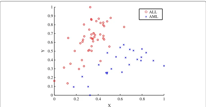
The properties of the diffraction-based clustering algorithm are illustrated using the [16] dataset. The data was normalised using the range as the scale measure and the minimum as the location measure [17]. Figure 1 shows thea prioriclassification of the samples, with the circle-markers indicating the acute lymphoblastic leukaemia (ALL) subtypes and the cross-markers indicating the acute myeloid leukaemia (AML) subtypes. The first two dimensions of the dataset are labelled using X and Y as seen in Figure 1.
0 0.2 0.4 0.6 0.8 1
0 0.1 0.2 0.3 0.4 0.5 0.6 0.7 0.8 0.9 1
ALL AML
X
Y
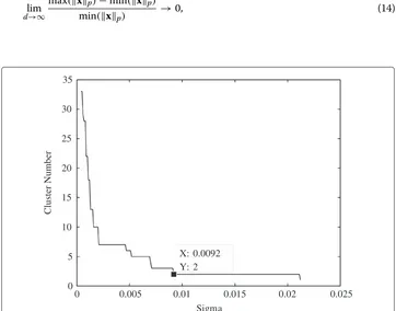
The diffraction-based clustering algorithm was applied to the filtered two dimensional Golub dataset for optimal results. The lifetime curve for the clustering algorithm in Figure 2 illustrates that the inherent number of clusters matches the expected amount. The value of σ was selected to be the minimum value of the range where the cluster number remains constant for the longest time, in this case the value ofσis 9.2×10⁻³.
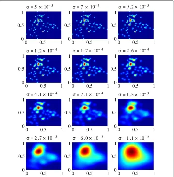
The evolution of the aperture function is shown in Figure 3 for increasingσvalues. The data points initially are point sources that slowly diffuse and merge to form larger clusters, which is depicted by the intensity change in Figure 3. The final result is that all the data points form a single cluster, a theme common to hierarchical clustering.
The cluster centres shown in Figure 4 are tracked asσ increases. The centres of the clusters move and merge to form new cluster centres, eventually leading to a single cluster centre. The route of the centre points is determined by the gradient and maxima of the aperture function which evolves as the parameterσchanges.
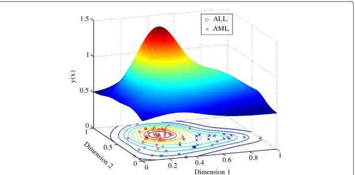
The final aperture function in Figure 5 has aσvalue determined from the cluster life-time plot and is used to classify the points into clusters. The aperture function has two peaks, one that is relatively higher than the other, which is a result of the higher density ALL data points. The number of clusters of dataset therefore correspond with the number of aperture peaks, which in this case is two.
Dimensionality reduction
Clustering algorithms often perform poorly in a high-dimensional space due to the rel-ative contrast between data points, x ∈ Rd, as expressed in the following equation
lim d→∞
max(xp)−min(xp) min(xp) →
0, (14)
0 0.005 0.01 0.015 0.02 0.025 0
5 10 15 20 25 30 35
X: 0.0092 Y: 2
Sigma
Cluster Number
0 0.5 1 0
0.5 1
0 0.5 1
0 0.5 1
0 0.5 1
0 0.5 1
0 0.5 1
0 0.5 1
0 0.5 1
0 0.5 1
0 0.5 1
0 0.5 1
0 0.5 1
0 0.5 1
0 0.5 1
0 0.5 1
0 0.5 1
0 0.5 1
0 0.5 1
0 0.5 1
0 0.5 1
0 0.5 1
0 0.5 1
0 0.5 1
σ= 5 × 10− 5 σ= 7 × 10− 5 σ= 9.2 × 10− 5
σ= 1.2 × 10− 4 σ= 1.7 × 10− 4 σ
= 2.6 × 10− 4
σ= 4.1 × 10− 4 σ= 7.1 × 10− 4 σ
= 1.3 × 10− 3
σ= 2.7 × 10− 3 σ= 6.0 × 10− 3 σ= 1.1 × 10− 2
Figure 3 Sigma evolution of the aperture function on the Golub dataset.The analysis of the Golub dataset was performed using a final selectedσ =9.2×10⁻³.
0 0.1 0.2 0.3 0.4 0.5 0.6 0.7 0.8 0.9 1 0 0.005 0.010 0.015 0.020 0.025 0.030 0.035 Dimension 1 σ σ
0 0.1 0.2 0.3 0.4 0.5 0.6 0.7 0.8 0.9 1 0 0.005 0.010 0.015 0.020 0.025 0.030 0.035 Dimension 2 ALL AML
0 0.2 0.4
0.6 0.8 1
0 0.5 10 0.5 1 1.5
Dimension 1
Dimension
2
y(
x
)
ALL AML
Figure 5 Aperture function of the Golub dataset atσ=9.2×10⁻³.The aperture function with its shape is used to classify the data points into two clusters.
where xp is the Lp norm [9]. The stated equation shows that the relative contrast between data points is degraded and has no meaning in a high-dimensional space. The high-dimensional feature space therefore needs to be reduced using an appropriate reduction technique.
Principal component analysis (PCA), as well as singular value decomposition (SVD), are both commonly used linear methods for reducing the dimensionality of the feature space. The linear methods construct a lower dimensional space using a linear function of the original higher dimensional space. A recent article written by Shi and Luo explored the use of a non-linear dimensionality technique on cancer tissue samples called isometric mapping (ISOMAP) [11]. ISOMAP replaces the usual Euclidean distance with a geodesic distance, which has the ability to capture and characterise the global geometric structure of the data [11]. The ISOMAP technique is also able to deal with non-linear relationships between data points as it is based on manifold theory [11].
The ISOMAP algorithm is applied to the cancer datasets to reduce their dimensionality. The dimension selected for each dataset is based on a paper by Tenenbaum which shows that the intrinsic dimensionality of the dataset can be estimated by the point of inflection, or “elbow” point, of the generated ISOMAP residual variance curve [18]. It should also be noted that Shi and Luo used a wide range of dimensions for thek-means and hierarchical clustering algorithm on the same cancer datasets used in this paper [11]. Their results show that the performance of the clustering algorithms for most of the cancer datasets remain relatively constant as the dimension changes [11].
Leukaemia dataset
The dataset is divided into two types one for training and one for testing the classifier. The initial training set contains 38 samples of which 27 are ALL and 11 are AML samples. The independent testing set contains 34 samples of which 20 are ALL and 14 are AML samples. The RNA was prepared from bone marrow mononuclear cells with the samples hybridised to a high-density oligonucleotide Affymetrix array containing 6 817 probes. The expression profile for each sample was then recorded and quantified using quality control standards [16].
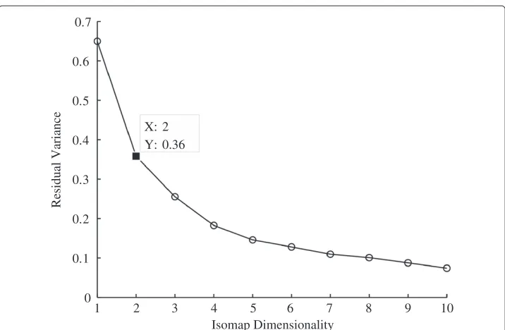
The Golub data was first filtered using the call markers to find genes that were present more than 1% out of all the samples. The dimensionality of the data was then reduced using the ISOMAP algorithm to a suitable dimension. The residual variance plot of the dataset, shown in Figure 6, reveals that the correct dimension is in fact two, as this is the dimension where the curve begins to approximate linear decay.
The performance of the clustering algorithms are evaluated using three main mea-sures: average external criterion (AEC), average validity index (AVI) and accuracy (ACC). The average external criterion is the average of the three main external criteria [17], and defined as
Average External Criterion= J+R+F
3 , (15)
where
J=Jaccard Coefficient,
R=Rand Score,
F=Folkes and Mallows Index.
1 2 3 4 5 6 7 8 9 10 0
0.1 0.2 0.3 0.4 0.5 0.6 0.7
X: 2 Y: 0.36
Isomap Dimensionality
Residual Variance
The average validity index is the average of four commonly used indices, analysed by [19], and is given by
Average Validity Index=
1
IB +ID+IC+I
4 , (16)
where
IB=Davies-Bouldin Index,
ID=Dunn’s Index,
IC =Calinski Harabasz Index,
I=I Index.
It is noted in (16) that the Davies-Bouldin index is inverted, since the index is minimised when there is a suitable clustering result. The average validity index should therefore be maximised for a good clustering result. It should be noted that other validation techniques exist which have been tested on numerous gene datasets [20,21].
The accuracy of the clustering results are determined using a simple misclassification ratio as shown by
Accuracy= Ns−Nm Ns ×
100%, (17)
whereNsis total number of samples andNmis the total number of misclassified samples produced by the algorithm.
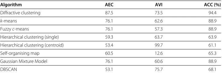
The results of the diffraction-based clustering algorithm were compared to the other main clustering schemes as shown in Table 1. Thek-means algorithm was used with the number of expected clusters equated to 2, similarly for the fuzzyc-means algorithm. The fuzzyc-means exponent was set to 2, the most commonly used value, however there are critiques about choosing this exponent value [22]. The hierarchical clustering algorithm used the standard Euclidean distance with single linkage and centroid linkage as the merg-ing measurement. The topology of the self-organismerg-ing map was 2×1, such that two cluster centroids could be found [16]. The number of clusters in the Gaussian mixture model and DBSCAN algorithm were set to 2.
The results in Table 1 demonstrate that the diffraction-based algorithm outperforms the other algorithms in terms of accuracy and validity. An accuracy of 94.4% for diffraction-based clustering implies that only 4 samples were misclassified, whereas in fuzzyc-means
Table 1 Comparison of the clustering results for the Golub dataset
Algorithm AEC AVI ACC (%)
Diffractive clustering 87.5 73.5 94.4
k-means 76.1 62.6 88.9
Fuzzyc-means 76.1 57.3 88.9
Hierarchical clustering (single) 59.3 63.7 63.9
Hierarchical clustering (centroid) 53.4 99.7 61.1
Self-organising map 60.5 12.6 65.3
Gaussian Mixture Model 76.1 60.6 88.9
DBSCAN 53.1 75.7 68.1
andk-means 8 samples were misclassified which is double that of the diffraction-based clustering algorithm.
The SOM and hierarchical clustering algorithms both perform relatively poorly com-pared to the other algorithms. The reason being that perhaps the incorrect choice of neurons and topology for the SOM was used, or the cut-off level for the hierarchical den-drogram was not optimal. The main problem with these algorithms is the choice for the parameters and determining the cluster numbera priori. The diffraction-based clustering algorithm bypasses these problems by finding the lifetime for the cluster numbers, which gives the optimal parameter choice for clustering the selected dataset.
MILEs dataset
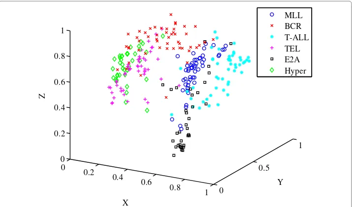
The Microarray Innovations in LEukaemia (MILE) study is a collection of analyses from an international standardisation programme that was conducted in 11 countries [23]. The subtypes of acute lymphoblastic leukaemia (ALL) which are analysed follow those from the study by Liet al. and include: t(4;11) MLL-rearrangement, t(9;22) BCR-ABL, T-ALL, t(12;21) TEL-AML1, t(1;19) E2A-PBX1 and Hyperdiploid>50 [24]. The lymphoblastic leukaemias result from the failed differentiation of the haematopoietic cells, specifically the lymphoid stem cells [23]. The number of samples were evenly distributed as much as possible resulting in 276 samples with a total of 54 675 genes.
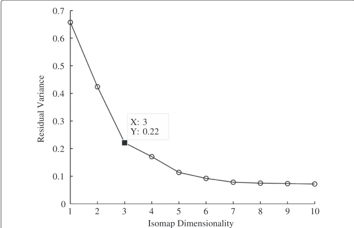
The dimensionality of the MILEs dataset was reduced to three using the ISOMAP algo-rithm and the information provided by the residual variance curve shown in Figure 7. The figure reveals that the inherent dimensionality is three as the curve begins to approximate linear decay at that point.
The data was background corrected and normalised using the robust multiarrary aver-age (RMA) technique. The data was then normalised again using the range such that the
1 2 3 4 5 6 7 8 9 10
0 0.1 0.2 0.3 0.4 0.5 0.6 0.7
X: 3 Y: 0.22
Isomap Dimensionality
Residual Variance
gene expression values were between [ 0, 1]. Thea prioriclassification of the dataset in Figure 8 shows each of the six subtypes designated by their own specific marker.
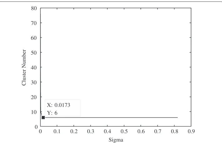
The lifetime curve for the Miles dataset is shown in Figure 9. The curve shows that the cluster number stays constant at six for a large range ofσ. The graph is not com-plete since the cluster number stays fixed at six for more than one order of magnitude inσ, and is therefore assumed to be the correct cluster number. The chosen value ofσ
is the minimum value at which the cluster number stays constant, which in this case is 17.3×10⁻³.
The results of the diffraction-based clustering algorithm were compared to the other clustering algorithms, as shown in Table 2. The number of expected clusters in thek -means algorithm was equated to 6, similarly for the fuzzyc-means algorithm. The fuzzy c-means exponent was set to 2. The hierarchical clustering algorithm uses the Euclidean distance with single linkage and centroid linkage as the merging metric at a maximum cluster level of six. The topology of the self-organising map was set to 6×1 such that six cluster centroids could be found. The number of clusters in the Gaussian mixture model and DBSCAN algorithm were set to 6.
The results in Table 2 show that the diffraction-based clustering algorithm outper-forms the other algorithms both in validity and accuracy. The fuzzyc-means algorithm is the closest, in terms of accuracy, to the diffraction-based clustering algorithm with a value of 71.4%. The accuracies in general are low when compared to the Golub dataset, with the reason being attributable to the large number of different subtypes and high-dimensionality of the feature space [9].
Other datasets
The cluster analysis of three other cancerous datasets was performed. Theσ parameter for the diffraction clustering algorithm was determined using the cluster lifetime curve.
0 0.2
0.4 0.6
0.8
1 0
0.5
1
0 0.2 0.4 0.6 0.8 1
MLL BCR T-ALL TEL E2A Hyper
X
Y
Z
0 0.1 0.2 0.3 0.4 0.5 0.6 0.7 0.8 0.9 0
10 20 30 40 50 60 70 80
X: 0.0173 Y: 6
Sigma
Cluster Number
Figure 9 Cluster lifetime plot for the three dimensional MILEs dataset.The lifetime plot illustrates how long a certain cluster size exists under evolution of theσparameter, and in this specific instance the cluster lifetime persists at 6 for a large range ofσvalues. The persistence of the line therefore indicates the correct cluster number is 6.
The parameters of the other clustering algorithms were adjusted to the correct number of clusters for each dataset.
Khan dataset
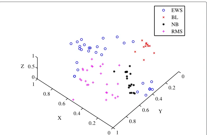
The Khan dataset was obtained from a study performed on classifying small, round blue-cell tumours (SRBCT) [25]. The tumours belong to four distinct diagnostic categories which present challenges for clinical diagnostics [25]. The four classes are Neuroblas-toma (NB), Rhabdomyosarcoma (RMS), Burkitt lymphomas (BL) and the Ewing family of tumours (EWS). The correct class to which the tumour belongs is important since treat-ment options, responses to therapy and prognoses vary significantly depending on the diagnosis [25].
The Khan gene-expression data was obtained from cDNA microarrays that each con-tained 6 567 genes, and a sample size of 83. The data was normalised to a range of [ 0, 1]
Table 2 Comparison of the clustering results for the MILEs dataset
Algorithm AEC AVI ACC (%)
Diffractive clustering 66.6 179.0 73.1
k-means 59.1 152.6 61.6
Fuzzyc-means 62.9 171.4 71.4
Hierarchical clustering (single) 47.7 64.2 47.1
Hierarchical clustering (centroid) 56.4 155.2 60.9
Self-organising map 46.1 10.6 47.1
Gaussian Mixture Model 58.6 96.4 61.2
DBSCAN 52.2 122.3 57.6
using the minimum as the location measure and the range as the scale measure. The dimensionality for the Khan dataset was originally selected as ten using PCA to allow for well-calibrated artificial neural network models [25]. The dataset however was reduced to three using the ISOMAP algorithm which is it’s intrinsic dimensionality. The predeter-mined classes of SRBCT tumours are shown in Figure 10. The sigma value was chosen to be 0.0099, which was obtained using the longest cluster lifetime.
The diffractive clustering algorithm was compared to the clustering algorithms for the Khan dataset, as shown in Table 3. The results show that the diffractive clustering algo-rithm is able to accurately separate the data into four distinct classes. The average external index of the diffractive clustering algorithm is also relatively higher indicating a suitable clustering solution.
The diffractive clustering algorithm was able to correctly classify 58 out of the 83 sam-ples as opposed to the fuzzyc-means algorithm which only correctly classified 54 out of the 83 samples, probably due to the fuzzyc-means algorithm finding a local minimum for its cost function as opposed to a global minimum.
Shipp dataset
The Shipp dataset is a study performed on diffuse large B-cell lymphoma (DLBCL), which is the most common malignancy in adults and is curable in less than 50% of cases [26]. The experiment performed by Shippet al.identified tumours in a single B-cell lineage, specifically the distinction of DLBCL from a related germinal centred B-cell follicular lymphoma (FL) [26]. The clinical distinction between the two types of lymphomas is usu-ally difficult as FLs acquire the morphology and clinical characteristics of DLBCLs over time [26]. The microrarray transcription study of the lymphomas, containing 6 817 genes,
0 0.2 0.4 0.6 0.8 1
0
0.2
0.4
0.6
0.8
1 0
0.5 1
EWS BL NB RMS
Y X
Z
Table 3 Comparison of the clustering results for the Khan dataset
Algorithm AEC AVI ACC (%)
Diffractive clustering 53.3 98.4 70.0
k-means 49.1 105.7 63.0
Fuzzyc-means 50.9 113.7 65.1
Hierarchical clustering (single) 40.7 79.8 43.2
Hierarchical clustering (centroid) 51.0 106.3 57.8
Self-organising map 46.3 15.7 54.2
Gaussian Mixture Model 51.8 102.2 50.6
DBSCAN 46.8 100.7 55.4
The diffractive clustering algorithm outperforms the other clustering algorithms in terms of accuracy, with the fuzzy
c-means algorithm performing well in terms of the validity index.
was performed on 77 patients, of whom 58 were diagnosed with DLBCL and other 19 with FL.
The dimensionality of the Shipp dataset was reduced to two dimensions using the ISOMAP algorithm. Thea prioriclassification of the 77 samples in two dimensions is shown in Figure 11. The similarity of the tumour lineage between DLBCLs and FLs is evident by the amount of mixing of the different data points, as shown in Figure 11. The sigma value was chosen to be 0.0073, which was obtained using the longest cluster lifetime.
The diffractive clustering algorithm, applied to the Shipp dataset, was compared to the other main types of clustering algorithms. The clustering results are shown in Table 4, with the most accurate and valid results pertaining to the diffractive clustering algo-rithm. The diffractive clustering algorithm correctly classifies 49 out of the 77 samples, as opposed to the SOM and hierarchical clustering algorithm which correctly classify only
0 0.2 0.4 0.6 0.8 1
0 0.1 0.2 0.3 0.4 0.5 0.6 0.7 0.8 0.9 1
DLBCL FL
X
Y
Table 4 Comparison of the clustering results for the Shipp dataset
Algorithm AEC AVI ACC (%)
Diffractive clustering 55.5 160.6 63.6
k-means 48.0 79.7 51.9
Fuzzyc-means 48.7 82.0 51.9
Hierarchical clustering (single) 51.1 112.2 53.3
Hierarchical clustering (centroid) 51.1 113.6 53.2
Self-organising map 47.7 14.7 53.3
Gaussian Mixture Model 49.8 66.8 51.9
DBSCAN 49.9 65.4 54.5
The diffractive clustering algorithm outperforms the others in terms of accuracy, however all the algorithms perform relatively poorly due to the mixing between the two different classes.
41 out of the 77 samples. The accuracy however of the diffractive algorithm, although 10% larger than the rest, is still relatively low.
Pomeroy dataset
The Pomeroy dataset is a study performed on embryonal tumours of the central ner-vous system (CNS) [27]. Medulloblastomas, a highly malignant brain tumour that originates in the cerebellum or posterior fossa, are most common in paediatrics with very little known about their response to treatment and pathogenesis [27]. The study performed by Pomeroyet al. analysed the transcription levels of 99 patients to iden-tify any expression differences between medulloblastomas (MED), primitive neuroec-todermal tumours (PNETs), atypical teratoid/rhabdoid tumours (AT/RTs), malignant gliomas (MAL) and normal tissue [27].
The Pomeroy study analyses the DNA from 99 patients on oligonucleotide microarrays with 6 817 genes. The data was also split into three datasets of varying sample size. The dataset known as A2 is used in this clustering analysis and contains 90 samples, of which 60 are MED, 10 are MAL, 10 are AT/RTs, 6 are PNETs and 4 are normal [27]. The dimen-sionality of the Pomeroy dataset was reduced to two using the ISOMAP algorithm. Thea prioriclassification of the samples using clinical methods is shown in Figure 12. The sigma value was chosen to be 0.00281, which was obtained using the longest cluster lifetime.
A cluster analysis was performed on the Pomeroy dataset using the diffractive clustering algorithm and compared to the other main types of clustering algorithms. The results are shown in Table 5, with the most accurate and valid results pertaining to the diffractive clustering algorithm. The diffractive clustering algorithm correctly classifies 61 out of the 90 samples as opposed to the hierarchical clustering algorithm which only classifies 51 out of the 90 samples correctly.
The validity of the clustering solution produced by the diffraction algorithm is also remarkably high compared to the other algorithms. The main reason for the accuracy of the diffraction algorithm being low, although still high relative to the other clustering results, is the unbalanced distribution of samples, which is a result of the large number of medulloblastoma samples in the dataset.
Discussion
0 0.2 0.4 0.6 0.8 1 0
0.1 0.2 0.3 0.4 0.5 0.6 0.7 0.8 0.9 1
MED MAL AT/RT Normal PNET
X
Y
Figure 12 Scatter plot of thea prioriclassification for the Pomeroy dataset.The five embryonal tumours of the central nervous system are shown. Medulloblastomas (MED), Primitive neuroectodermal tumours (PNETs), Atypical teratoid/rhabdoid tumours (AT/RTs), Malignant gliomas (MAL) and Normal tissue.
the hierarchical clustering algorithm, self-organising map, Gaussian mixture model and DBSCAN require initialisation of parameters and layouts which can often lead to poor results.
Another difficulty associated with conventional clustering algorithms is deciding on correct number of clusters to select. There are however techniques, such as the gap statis-tic, which allows one to estimate the correct number of clusters [28]. The problem with the gap statistic is the choice of the reference distribution, which if chosen to be uniform produces ambiguous results for elongated clusters [28]. There are other more robust tech-niques that can be combined with the algorithms, such as robustness analysis and cluster ensembles, which can determine the correct number of clusters [29,30].
Resampling-based methods can also be used in conjunction with conventional cluster-ing algorithms to improve their performance [31]. By contrast, the algorithm presented in
Table 5 Comparison of the clustering results for the Pomeroy dataset
Algorithm AEC AVI ACC (%)
Diffractive clustering 63.1 258.7 67.8
k-means 42.7 173.6 48.9
Fuzzyc-means 39.9 154.6 43.3
Hierarchical clustering (single) 49.8 256.2 56.7
Hierarchical clustering (centroid) 50.7 292.6 57.8
Self-organising map 41.2 13.7 44.4
Gaussian Mixture Model 42.2 79.2 37.7
DBSCAN 36.6 46.4 33.3
this paper can inherently determine the correct cluster number using the cluster lifetime. The merit of the diffractive clustering algorithm is therefore due first to the ability of the algorithm to handle non-spherical or arbitrarily shaped clusters, and secondly due to the optimisation of its single parameter,σ, using the cluster lifetime.
Conclusion
The recent development in microarray technology has given rise to a large amount of data on the genetic expressions of cells. A solution to this problem of discovery and analysis in gene expression data is the application of unsupervised techniques such as cluster anal-ysis. The clustering of samples allows one to find the inherent structure in the genome without filtering or representing the data with only a few selected genes.
The validation and performance of the clustering results, although poorly defined, can be addressed successfully with relative and external criteria. The number of clustering algorithms is large and as such the choice of the correct or preferred algorithm remains ambiguous. The languid approach is usually to choose the fastest algorithm such as the k-means algorithm. The classical algorithms although fast lack the insight to the cluster-ing process, and rely on the predetermined, usually biased number of clusters to work. The diffractive clustering algorithm is independent of the number of clusters as the algo-rithm searches the feature space and requires no other form of feedback. The results also show that the diffractive clustering algorithm, in terms of accuracy, outperforms the other classical types of clustering algorithms.
Competing interests
The authors declare that they have no competing interests.
Authors’ contributions
SD proposed the diffraction approach, developed the algorithm, performed its implementation and carried out the research. MV helped supervise the project and provided consultation on related pattern analysis and classification matters. SC helped with the medical aspects of the project and also with obtaining the microarray data. DR formulated the general project, supervised the research, coordinated the biomedical and engineering aspects, and contributed to editing the manuscript. All authors read and approved the final manuscript.
Acknowledgements
This work is funded by Fogarty International Center grants for HIV-related malignancies (D43TW000010-21S1) and TB (5U2RTW007370-05). The opinions expressed herein do not necessarily reflect those of the funders.
Author details
1Biomedical Engineering Research Group in the School of Electrical & Information Engineering, University of the Witwatersrand, Johannesburg, South Africa.2Systems & Control Research Group in the School of Electrical & Information Engineering, University of the Witwatersrand, Johannesburg, South Africa.3National Health Laboratory Service and Department of Molecular Medicine and Haematology, University of the Witwatersrand, Johannesburg, South Africa.
Received: 13 August 2012 Accepted: 12 November 2012 Published: 19 November 2012
References
1. Cobb K:Microarrays: The Search for Meaning in a Vast Sea of Data.Tech. rep., Biomedical Computation Review 2006.
2. Statnikov A, et al.:A comprehensive evaluation of multicategory classification methods for microarray gene expression cancer diagnosis.Bioinoformatics2005,21(5):631–634.
3. Domany E:Cluster Analysis of Gene Expression Data.J Stat Physcs2003,110(3–6):1117–1139. 4. Jiang D, et al.:Cluster Analysis for Gene Expression Data: A Survey.IEEE Trans Knowledge Data Eng2004,
16(11):1370–1386.
5. Frey BJ, Dueck D:Clustering by Passing Messages Between Data Points.Science2007,315:972–976. 6. Dr˘aghici S:Data Analysis Tools for DNA Microarrays. London: Chapman & Hall/CRC Mathematical Biology and
Medicine Series; 2003.
7. Belacel N, et al.:Clustering Methods for Microarray Gene Expression Data.J Integrative Biol2006,10(4):507–531. 8. Sorlie T, et al.:Gene Expression Patterns of Breast Carcinomas Distinguish Tumor Subclasses with Clinical
9. Aggarwal CC, et al.:On the Surprising Behaviour of Distance Metrics in High Dimensional Space.Lecture notes, Institute of Computer Science, University of Halle 2001.
10. Yeung KY, Ruzzo WL:Principal Component Analysis for Clustering Gene Expression Data.Bioinformatics2001,
17(9):763–774.
11. Shi J, Luo Z:Nonlinear dimensionality reduction of gene expression data for visualisation and clustering analysis of cancer tissue samples.Comput Biol Med2010,40:723–732.
12. Fowles GR:Introduction to Modern Optics. 2nd edition. New York: Dover Publications; 1975.
13. Roberts SJ:Parametric and Non-parametric Unsupervised Cluster Analysis., Technical Report 2, 1997. 14. Leung Y, et al.:Clustering by Scale-Space Filtering.IEEE Trans Pattern Anal Machine Intelligence2000,
22(12):1396–1410.
15. Yao Z, et al.:Quantum, Clustering Algorithm based on Exponent Measuring Distance.InInternational Symposium on Knowledge Acquisition and Modeling Workshop, 2008. KAM Workshop 2008,IEEE Catalog Number 10560087, IEEE; 2008:436–439. [ISBN 978-1-4244-3530-2].
16. Golub TR, et al.:Molecular Classification of Cancer: Class Discovery and Class Prediction by Gene Expression Monitoring.Science1999,286:531–537.
17. Gan G, et al.:Data Clustering Theory, Algorithms, and Applications. Philadelphia: SIAM, Society for Industrial and Applied Mathematics; 2007.
18. Tenenbaum JB, de Silva V, Langford JC:A global geometric framework for nonlinear dimensionality reduction. SCIENCE2000,290:2319–2323.
19. Maulik U, Bandyopadhyay S:Performance Evaluation of Some Clustering Algorithms and Validity Indices.IEEE Trans Pattern Anal Machine Intelligence2002,24(12):1650–1654.
20. Datta S, Datta S:Comparisons and validation of statistical clustering techniques for microarray gene expression data.Bioinformatics2003,19(4):459–466.
21. Handl J, Knowles J, Kell DB:Computational cluster validation in post-genomic data analysis.Bioinformatics
2005,21(15):3201–3212.
22. Dembele D, Kastner P:Fuzzy c-means method for clustering microarray data.Bioinformatics2003,19(8):973–980. 23. Mills K, et al.:Microarray-based classifiers and prognosis models identify subgroups with distinct clinical
outcomes and high risk of AML transformation of myelodysplastic syndrome.Blood2009,114(5):1063–1072. 24. Li Z, et al.:Gene Expression-Based Classification and Regulatory Networks of Pediatric Acute Lymphoblastic
Leukemia.BLOOD2009,114(20):4486–4493.
25. Khan J, Wei JS, Ringnér M, et al.:Classification and Diagnostic Prediction of Cancers using Gene Expression Profiling and Artificial Neural Networks.Nat Medicine2001,7(6):673–679.
26. Shipp MA, Ross KN, Tamayo P, et al.:Diffuse Large B-cell Lymphoma Outcome Prediction by Gene Expression Profiling and Supervised Machine Learning.Nat Medicine2002,8:68–74.
27. Pomeroy SL, Tamayo P, Gaasenbeek M, et al.:Prediction of Central Nervous System Embryonal Tumour Outcome Based on Gene Expression.Nat Medicine2002,415:436–442.
28. Tibshirani R, Walther G, Hastie T:Estimating the number of clusters in a data set via the gap statistic.R Stat Soc
2001,63(2):411–423.
29. Gallegos MT, Ritter G:A robust method for cluster analysis.Ann Stat2005,33:347–380.
30. Strehl A, Gosh J:Cluster ensembles–A knowledge reuse framework for combining multiple partitions. J Machine Learning Res2002,3:583–617.
31. Monti S, Tamayo P, Mesirov J, Golub T:Consensus clustering: a resampling-based method for class discovery and visualization of gene expression microarray data.Machine learning2003,52:91–118.
doi:10.1186/1475-925X-11-85
Cite this article as:Dingeret al.:Clustering gene expression data using a diffraction-inspired framework.BioMedical Engineering OnLine201211:85.
Submit your next manuscript to BioMed Central and take full advantage of:
• Convenient online submission
• Thorough peer review
• No space constraints or color figure charges
• Immediate publication on acceptance
• Inclusion in PubMed, CAS, Scopus and Google Scholar
• Research which is freely available for redistribution