The Thirty-Third AAAI Conference on Artificial Intelligence (AAAI-19)
Re
2EMA: Regularized and Reinitialized Exponential
Moving Average for Target Model Update in Object Tracking
Jianglei Huang, Wengang Zhou
CAS Key Laboratory of Technology in GIPAS, EEIS Department, University of Science and Technology of China [email protected], [email protected]
Abstract
Target model update plays an important role in visual object tracking. However, performing optimal model update is chal-lenging. In this work, we propose to achieve an optimal tar-get model by learning a transformation matrix from the last target model to the newly generated one, which results into a minimization objective. In this objective, there exists two challenges. The first is that the newly generated target model is unreliable. To overcome this problem, we propose to im-pose a penalty to limit the distance between the learned target model and the last one. The second is that as time evolves, we can not decide whether the last target model has been corrupted or not. To get out of this dilemma, we propose a reinitialization term. Besides, to control the complexity of the transformation matrix, we also add a regularizer. We find that the optimization formula’s solution, with some simplifi-cations, degenerates to EMA. Finally, despite the simplicity, extensive experiments conducted on several commonly used benchmarks demonstrate the effectiveness of our proposed approach in relatively long term scenarios.
Introduction
Visual object tracking is a fundamental task of computer vi-sion and has many practical applications such as in moni-toring and auto-driving (Smeulders et al. 2014; Zhang et al. 2015; Wu, Lim, and Yang 2013; Han, Sim, and Adam 2017; Wang et al. 2018; Wang, Zhou, and Li 2018a; 2018b). The objective of object tracking is to online locate an arbitrary target with only initial object’s bounding box given, which implies that there is no prior information about the target in the offline phase. This requires that the target’s model should be online constructed from the given bounding box and updated on the fly with predicted ones in successive video frames. Therefore, model update plays a crucial role in object tracking algorithms.
However, in visual object tracking, model update is chal-lenging, since there are distractors and other corrupted situa-tions such as occlusion and blur. The target model generated based on the current video frame may be unreliable, which risks corrupting the initial model when used for updating. Besides, what is even worse is the accumulation of small er-rors. The small errors such as background pixels included
Copyright c2019, Association for the Advancement of Artificial Intelligence (www.aaai.org). All rights reserved.
in the bounding box may accumulate with continuously up-dating, which will eventually degrade the target model and make the tracker drift away. The big corruption sources may be eliminated by some specialized techniques such as oc-clusion and/or blur detection, but the accumulation of small errors is hard to avoid.
Recently, there have been works (Bertinetto et al. 2016a; 2016c; Tao, Gavves, and Smeulders 2016) that explore the possibility of performing no model update at all. In those methods, visual object tacking is formulated as an one-shot learning problem. Despite the simplicity, encouraging re-sults are achieved. Essentially, those methods learn to derive a general model regardless of target variations with large of-fline datasets. In principle, they intend to learn an invariant and discriminative feature extractor such that the target is stable and separable from background in the feature space (Li et al. 2018). However, learning such an extractor that can produce an invariant and discriminative representation is in-trinsically difficult. Because as time evolves, the appearance of the target may change drastically and even become irrel-evant with that of the given sample. For example, initially given a frame containing a closed book, when it is opened up in successive frames, its appearance becomes irrelevant. As a result, those methods may fail to extract a relevant fea-ture and eventually lose the target. If there is model update, those kind of failure could be avoided. Besides, with model update, we may be free of the large scale datasets for offline training in those algorithms.
The most popular update policy is exponential moving av-erage (EMA). This approach basically adds up all online col-lected training samples with an exponential decayed weight for each sample. It can be implemented in a “moving” man-ner, and thus there is no need to keep the historical samples. Therefore it can be both memory and computation efficient. However, it is ad-hoc and its effect is limited. In this work, we seek a more complicated update method.
update rate. In other words, the naive EMA can be inter-preted in an optimization point of view, which serves as a new insight into EMA. In other literatures, the effectiveness of EMA is interpreted in a aggregation theory point of view (Bolme, Draper, and Beveridge 2009). In addition to this, with the convenience of this math formula representation, we can easily incorporate other terms into this objective.
The first term is the regularization, which seems trivial but in our experiments we find that it has positive effect on the performance. In addition, because of its existence, we can apply other advanced techniques such as kernel trick (Hen-riques et al. 2015).
The second one is the reinitialization. The above objective can also be interpreted in a manifold learning perspective, i.e., the target models at different time-steps form a man-ifold path, and our learned target model must keep close enough to the endpoint of the manifold path while adapt-ing to the target model newly generated in the current video frame. However, as time evolves, the manifold path becomes very long and the endpoint is far away from start point. Then there comes an ambiguity dilemma. On the one side, the sit-uation, i.e., the large distance between the start point and endpoint, is reasonable, because that the target appearance may have largely changed and we need to adapt to it. On the other side, this occasion should be avoided, and we need to return to the start point, as the endpoint may have been corrupted by small errors’ accumulation or other big pollu-tion sources. We can not decide which side the real case is. Inspired by the solution in PageRank (Page et al. 1999) algo-rithm, we propose to randomly select one side to jump out of this dilemma. Further, since the random solution is not deterministic, we take a weighted hybrid decision instead.
In summary, we propose an optimization objective for tar-get model update, which can be degenerated with some sim-plifications to EMA. With the convenience of this fashion, it is flexible to incorporate regularization term and further apply other advanced techniques such as kernel trick. In ad-dition, to overcome the degradation of the target model, we also propose a reinitialization term. Finally, our method can take place of EMA seamlessly, which will further bring per-formance improvement.
Related Work
In this section, we mainly introduce related tracking algo-rithms on model update. For a more comprehensive sur-vey, interested readers can refer to (Yilmaz, Javed, and Shah 2006; Smeulders et al. 2014; Kristan et al. 2016).
EMA.Averaging of filters is first employed in (Bolme, Draper, and Beveridge 2009), which is motivated by the ag-gregation theory,i.e., bagging. Particularly, the exact filters can be viewed as weak classifiers, the averaging of which can form a stronger classifier. Later in (Bolme et al. 2010), the averaging is adopted in an online vision, where the his-torical filters’ weights are exponential decayed, thus this variant is called exponential moving average (EMA). Since then, EMA is broadly utilized in correlation filter related object tracking algorithms (Henriques et al. 2015). Recent years, it has been found that EMA can also be employed in Siamese network related tracking methods (Valmadre et
al. 2017). We propose to minimize a square error to learn a best transformation matrix, motivated by the fact that the target model need to adapt to the variation of the object and the newly generated target model is unreliable. We find the solution of this formula’s base form equals to EMA, which implies that EMA can be interpreted in an optimization point of view.
Imposing Restrictions on Model Update.There is a crit-ical problem related to stability-plasticity dilemma in model update (Li et al. 2018). On the one hand, model update should be plastic to effectively absorb new variations from tracked target. On the other hand, it needs to be stable to avoid being corrupted when small errors accumulate. Note that there are differences between the dilemma explained here and the one described by us. The former is a common plight in model update, in contrast, the later is a situation that we do not know which action to perform when the manifold path is far away from the start point. In the other words, the later is more specific than the former.
To alleviate this problem, Lainet.al.keep the initial tar-get model as a reference, and they update to the latest tartar-get model only when its predicted parameters are close enough to those learnt by the reference model (2004). They take a threshold to decide whether it is close enough. Similar meth-ods are taken in (Guo et al. 2017) that learns a transform matrix from the initial target model directly to the latest one. Inspired by those two, Liet.al.adopt an anchor loss while training their GRU based model update module (2018).
Those techniques are intrinsically similar with the reini-tialization term employed by us,i.e., all of them follow the principle that limits the manifold path not to go too far away form the start point. But, their specific practices are differ-ent. Facing the ambiguity dilemma, we propose to randomly select one way to jump out, and later to make it practical, we take a hybrid decision. Besides, our method can be viewed as a re-weighting process, which up-weights the initial tar-get model adaptively as the manifold path grows. In contrast, above techniques limits the distance by a threshold control-ling the nearness between two groups of predicted parame-ters, a transforming matrix only from the initial model to the latest one, or an anchor loss in offline training process.
its applications in real-time situations. Our reinitialization term can also be viewed as a re-weighting process as men-tioned above, but it only re-weights two weights,i.e., one for the initial target model and the other for the latest target model, which brings little computation overhead.
Short- and Long-term Memory.A mixture model con-sisting of three components,i.e., a stable component respon-sible for long-term variations, a two-frame transient compo-nent for capturing short-term variations, and an outlier pro-cess is proposed in (Jepson, Fleet, and El-Maraghi 2003). Inspired by Atkinson-Shiffrin Memory Model, Honget.al. propose to form a short-term store and a long-term store to collaboratively process the object tracking task (2015).
RNNs Based Model Update Modules.Yang and Chan propose a LSTM memory module to cope with model update problem for Siamese network based methods (2017). How-ever, this memory module barely brings improvement on the performance. Later in (Yang and Chan 2018), they provide an improved version, where the LSTM no longer acts as the memory module but serves as a memory controller, which controls the assembling, reading and writhing of candidate target models. The improved version shows its effectiveness in various of benchmarks. In (Li et al. 2018), a GRU based meta-learner for learning how to update the target model is proposed. This approach shares some similarities with Yang and Chan’s method, but during offline training they utilize an anchor loss, which is crucial for successfully learning.
Methods
Primal Objective
In the online tracking process, when a new frame comes, a typical model matching based object tracking algorithm first detects the most similar region with the target model. Next based on the detected region it generates a new target model, then with which it updates the original target model. The most commonly used update policy is exponential moving average (EMA),
Tt= (1−η)Tt−1+ηEt, (1)
whereTtdenotes the learned target model in time stept,Et
is the naive target model generated purely from the detected region in frametandηis the update rate.
EMA can be viewed as a linear interpolation between cur-rent and historical target models, and the weights of past tar-get models are exponential decayed. The update process in EMA can be highly efficient since it needs no iterative opti-mization nor extra memory. However, this method is ad-hoc and can hardly handle more complex situations such as oc-clusion and blur. Instead, we seek a more complicated and effective method to update the target model. We propose fol-lowing optimization objective,
W0=argmin
W
{||Tt−1∗W−Et||2+
λ||Tt−1∗W−Tt−1||2+µ||W||2},
(2)
where∗ denotes circular convolution,λis the penalty fac-tor and µis the regularizer. Eq. 2 learns an optimal trans-formation matrixW0 from the previous target modelTt−1
Figure 1: Illustration of our method. Each point denotes the target model T at different time steps. Those target mod-els form a manifold path. The objective of our method is to learn aTtwhich adapts to the newly generated target model Etwhile keeping close enough toTt−1. When the manifold
path becomes long, as indicated by the color, we can not de-cide whetherTt−1has been corrupted or not. Therefore we
could either return toT0by chance (a) or take a mixture of T0andTt−1(b) to get out of this dilemma.
to approximate the newly generated target model Et. The
newly generated target modelEtis not reliable, as there are distractors and occlusion, thus we add a penalty in Eq. 2 to force the learned target model not to change too much from the previous target modelTt−1. Finally, the current target
model can be obtained by
Tt=Tt−1∗W0. (3)
Ambiguity Dilemma
Eq. 2 can be interpreted in a manifold learning point of view as illustrated in Fig. 1 (a). We want to learn an optimal target modelTtbetweenTt−1andEtsuch that it is close enough
toEtto capture the appearance variations of the target, as
well as not too far away fromTt−1 to ensure the
smooth-ness of the manifold path. In other words, we need to find the best location ofTtin order to minimize the distance be-tweenTt−1andEtwith a distance weightλcontrolling the
smoothness of the manifold path.
In this light, as tracking proceeds, there occurs an ambi-guity dilemma. There exists at1, whent > t1, the manifold
would go sufficiently far away form the start pointT0. This
may attribute to two reasons: (a) the appearance of the target has significantly changed and (b) the target modelTt−1 is
corrupted by non-target pixels such as background.
The first case is reasonable, and we may continue to com-pute the target model Tt along the manifold path. On the
contrary, the second case should be avoided, since the cur-rent manifold path is corrupted, and we need to create a new path. In the task of object tracking, the most reliable target model is T0 as it is given. Thus under the second
manifold path. However, the problem is that when the dis-tance betweenT0andTt−1is sufficiently large, there is no
way to know which case it belongs to. Therefore we could not decide which action to perform.
Random-walk Reinitialization
To jump out of above dilemma, we could randomly select one action to perform, which process is illustrated in Fig. 1 (a). In PageRank algorithm (Page et al. 1999), there is a sim-ilar dilemma, where there are loops among web page while computing the rank. Lawrenceet.al.offer chances to jump out of those loops. In our problem, we could perform in a similar way to decide whether to continue to walk along the manifold path or just return to the start point. Formally, we add a reinitialization term in Eq. 2 as follows,
W0=argmin
W
{||Tt−1∗W−Et||2+
λ((1−I(p))||Tt−1∗W−Tt−1||2+
I(p)||Tt−1∗W−T0||2) +µ||W||2},
(4)
whereI(p) = 1with some probabilityp.
Weighted Hybrid Decision
Eq. 4, however, is not applicable. Since it randomly chooses one action to perform in every time step while updating the target model, its result is not deterministic, which is fatal in real applications. To deal with the problem, we could take a mixture ofT0andTt−1, which is stated in Fig.1 (b).
For-mally, we defineg(p)as a map ofpto replaceI(p), where
g(p)∈ {x|x∈Randx∈[0,1]}. Then Eq. 4 becomes
W0=argmin
W
{||Tt−1∗W−Et||2+
λ((1−g(p))||Tt−1∗W−Tt−1||2+
g(p)||Tt−1∗W−T0||2) +µ||W||2}.
(5)
Eq. 5 is deterministic, and thus it is applicable in practical applications, and in some way it overcomes the target model degradation problem.
We definepas a metric ofTt−1andT0 to measure the
length of the manifold path. Specifically, in this paper we take cosine distance asp,i.e.,
p= 1− |ver(T0)
Hver(T t−1)|
p
(ver(T0)Hver(T0))(ver(Tt−1)Hver(Tt−1))
,
(6) wherever()denotes the vectorization operation, andTHis the Hermitian transpose ofT,i.e.,TH= (T∗)TandT∗is the
complex conjugate ofT.
We defineg(p)as a power function to properly weight the two side of the ambiguity dilemma. When the manifold path is short,i.e.,pis small, the target model should aggressively adapt to the change of the target appearance, and thusg(p)
should be small. In contrast, when the manifold path is long, i.e.,pis large, the target model may be corrupted and we should up-weight the initial target modelT0, which requires
largeg(p). Therefore,g(p)should be positive related top
and in this work we setg(p)as
g(p) =
(αp)k, if(αp)k
61,
1, if(αp)k >1, (7)
whereα >0andk>1are hyper-parameters.
Solution
Primal Solution. Since Eq. 5 is convex, we can derive a closed form solution. In most of tracking algorithms,Tt ∈
Rn. We could convert andimensional tensor to an one
di-mensional vector by vectorization operation. Therefore in the following, we take the one dimensional vector to derive the solution and use lower case to represent for correspond-ing vectors. LetXtbe a matrix containing all circulant shifts ofttas is in (Henriques et al. 2015), then Eq. 5 becomes,
w0=argmin
w
{||Xt−1w−et||2+
λ((1−g(p))||Xt−1w−tt−1||2+
g(p)||Xt−1w−t0||2) +µ||w||2}.
(8)
To findw0, define
l=||Xt−1w−et||2+λ((1−g(p))||Xt−1w−tt−1||2 +g(p)||Xt−1w−t0||2) +µ||w||2.
(9)
Setting ∂w∂l =0, we have the solution,
w0 =((1 +λ)XTtXt+µI)−1XTt( et+λ((1−g(p))tt−1+g(p)t0)).
(10)
However, above equation needs to compute large matrix’s inversion, which is known time-consuming, therefore we should find other alternatives. Following (Henriques et al. 2015), by using the circulant matrix’s property,
Xt=Fdiag(ˆtt−1)FH, (11)
whereFis the DFT matrix, and the hatˆdenotes the DFT of a vector, the solution can be derived as
ˆ
w=ˆtt−1(ˆet+λ((1−g(p))ˆtt−1+g(p)ˆt0))
(1 +λ)ˆt∗t−1ˆtt−1+µ , (12)
wheredenotes the element-wise multiplication andˆt∗t−1
is the complex conjugate ofˆtt−1.
Kernelization. The kernel trick can also be applied as with (Henriques et al. 2015). Specifically, expressingwas
w=X
i
αiϕ(tit−1), (13)
wheretit−1 is theith row of circulant matrixXt−1, we can
find
ˆ
α=ˆet+λ((1−g(p))ˆtt−1+g(p)ˆt0) (1 +λ)ˆktt−1tt−1+µ
, (14)
where the hatˆagain denotes DFT andktt−1tt−1 is the first row of the kernel matrixKwith elements
Kij =k(tit−1,tjt−1) =ϕT(tit−1)ϕ(tjt−1). (15) Then the target modelttcan be written as
ˆtt=kˆ tt−1tt−1
(ˆet+λ((1−g(p))ˆtt−1+g(p)ˆt0))
(1 +λ)ˆktt−1tt−1+µ
. (16)
Finally, we can perform IDFT to convertˆttback to its
Relationship with EMA
In Eq. 16, settingµ= 0andg(p) = 0, we will get
ˆtt=ˆet+λˆtt−1
1 +λ . (17)
DFT has linear property (Gonzalez and Woods 2001), there-fore Eq. 17 equals to
tt= λ
1 +λtt−1+
1
1 +λet, (18)
which is the same with EMA in Eq. 1 with η = 1+1λ. In other words, our method can be viewed as an extension of EMA with regularization and reinitialization, and we name our method asRe2EMA.
Experiments
In this section, we first provide a comprehensive study about our method. After that we present comparison results with other related object tracking algorithms.
Experimental Setups
Implementation Details.As a common practice with cor-relation filters, to employ the cyclic assumption, we need to weightTt−1,T0, andE0by a cosine window to convert
them to Fourier domain (Henriques et al. 2015). For correla-tion filter related algorithms, the target models are already in Fourier domain, thus we could directly take Eq. 16 to get the solution. But for Siamese network related methods, the tar-get models are originally in spatial domain. To convert them to Fourier domain, we need to multiply a cosine window. However, this operation will cause an information loss. To overcome this problem, we setµ= 0in Eq. 16 to get
ˆ Tt=
ˆ
Et+λ((1−g(p))ˆTt−1+g(p)ˆT0)
1 +λ . (19)
As mentioned earlier, DFT has linear property, then Eq. 19 becomes
Tt=Et+λ((1−g(p))Tt−1+g(p)T0)
1 +λ . (20)
The above equation is in spatial domain, and we could em-ploy it in Siamese network related algorithms. Note that ac-tually Eq. 20 discards the regularization term, which is a compromise to the information loss limitation.
Evaluation Metrics. For OTB family (Wu, Lim, and Yang 2015) and TColor-128 (Liang, Blasch, and Ling 2015) datasets, we take one-pass evaluation (OPE) with precision and success plots metrics. The precision plot measures the distance between the predicted and the ground-truth cen-ter locations under different thresholds (at a threshold 20 is called DP). The success plot measures the overlap ratios of the predicted and the ground-truth bounding boxes, where the area under the curve (AUC) is computed as an overall performance measurement.
Methods AUC (%)
BACF (2017) 63.24
Reg. Rei.
BACF Re2EMA
7 7 62.77
3 7 62.85
7 3 64.76
3 3 65.18
kernel
linear 65.18 Gaussian 65.22 polynomial 65.42
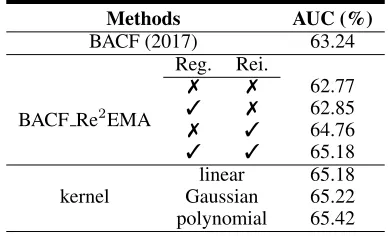
Table 1: Ablation study of proposed regularization and reini-tialization terms, with performances of different kernels. Reg.: regularization term. Rei.: reinitialization term.
Ablation Study
In this subsection, we take OTB-2015 (Wu, Lim, and Yang 2015) as a validation set and BACF (Galoogahi, Fagg, and Lucey 2017) as a baseline method to analyze each proposed component. Note that BACF already employs EMA to up-date their target model, therefore considering the relation-ship of EMA and our method Re2EMA, we setλ≈ 1
η −1,
and only tuneµ,αandkin OTB-2015.
Regularization and reinitialization term are effective.
Table 1 shows the ablation analysis of the proposed two terms. With both terms, our method is 1.94% better than BACF baseline, which is a significant improvement. To in-vestigate the source of this improvement, we conduct several experiments. Firstly, to ensure that the improvement does not come from any other resources,e.g., λor the form of the formula, we run our method without both terms, which leads to 62.77% in AUC. This result is a little lower than that of EMA, which two in our expectations should be the same, since our method in the simplest form equals to EMA. This is due to the update rateη is0.013, and in our method we setλ= 76.0for numerical propose,i.e.,λdoes not strictly equal to 1η−1. Next, we run our method with only the regu-larization term, and it results in 62.85%, which suggests that regularization term has positive effect on performance but is not the main contributor. Finally, we run our approach with only the reinitialization term to get 64.76% in AUC, which indicates that the reinitialization term contributes most to the improvement of performance.
The above ablation experiments clearly show that the reinitialization term proposed by us has a great impact on the tracking results, which also indicates that the degrada-tion of target model is a severe problem in model update.
OTB-2015 OTB-50 TColor-128
Methods speed DP AUC DP AUC DP AUC
(fps.) (%) (%) (%) (%) (%) (%)
KCF 236 69.66 48.46 61.06 40.70 55.79 39.18 +Re2 239 71.71 49.30 62.07 41.42 56.01 39.58 ∆ +2.05 +0.84 +1.01 +0.72 +0.22 +0.40 Staple 39 77.50 58.63 66.26 50.60 66.42 50.49 +Re2 29 82.03 62.26 72.73 54.60 69.50 52.01
∆ +4.53 +3.63 +6.47 +4.00 +3.08 +1.52
SRDCF 6 77.63 60.19 70.42 53.60 65.08 48.83 +Re2 6 80.07 62.55 72.88 55.50 66.42 50.14 ∆ +2.44 +2.36 +2.46 +1.90 +1.34 +1.31 BACF 16 82.37 63.24 76.82 58.04 65.87 50.20 +Re2 15 83.21 65.18 78.81 60.75 66.45 51.33
∆ +0.84 +1.94 +1.99 +2.71 +0.58 +1.13
SiamFC 29 76.79 59.49 67.93 52.14 69.40 50.74 +Re2 30 80.14 62.24 72.03 55.43 70.99 51.89 ∆ +3.35 +2.75 +4.10 +3.29 +1.59 +1.15
CFNet 27 73.86 57.02 68.63 51.88 60.91 45.78 +Re2 30 76.04 59.08 68.97 52.36 61.83 46.30 ∆ +2.18 +2.06 +0.34 +0.48 +0.92 +0.52
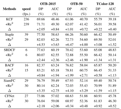
Table 2: Experiment results of before and after applying Re2EMA on several benchmarks. ∆ denotes the perfor-mance gain. +Re2 means taking Re2EMA as the target model update method in baseline tracking algorithms. The speed is averaged on TColor-128 dataset.
find that in KCF (Henriques et al. 2015) Gaussian kernel performs worst and linear kernel behaves similar with poly-nomial kernel. Therefore, to ensure efficiency and effective-ness, we prefer linear kernel and take it as a default option for all our experimented tracking approaches.
Map functiong(p)is important.We plot the optimized
g(p)in Fig. 2, from which we find g(p)is similar with a threshold decision function,i.e.,
q(p) =u(p−a) =
0, ifp < a,
1, ifp>a, (21)
whereais a threshold andu(p−a)is the shifted unit step function. Thereforeg(p)can be viewed as a soft threshold decision function. Then how does q(p)perform? We find that employingq(p)results in 63.16% in AUC, which is 2.02 percentage points lower than that of g(p) (65.18%). This comparison result suggests that a soft decision function is much better. From the Fig. 2, we can also find that the tran-sition point when the function value first becomes 1 ofg(p)
(P1in Fig. 2) arrives earlier than that (P2in Fig. 2) ofq(p).
An explanation to this phenomenon is that at the same level of corruption of the componentEt, the algorithm should
re-turn toT0. Since in our method we apply a soft threshold
decision functiong(p),i.e., we allow a larger proportion of
T0earlier, to arrive at the same level corruption ofEtwith
that in usingq(p), the transition point should come earlier.
Baseline Comparisons
In this section, we select some representative trackers from both correlation filter and Siamese network families as our baseline methods. From correlation filter family, we
Figure 2: Plot ofg(p)and threshold decision functionq(p).
g(p)can be viewed as a soft threshold decision function.
Figure 3: Precision and success plots on OTB-2015. Only top 10 trackers are shown. The legend on the left figure con-tains DP, while on the right is AUC instead.
choose KCF (Henriques et al. 2015), Staple (Bertinetto et al. 2016b), SRDCF (Danelljan et al. 2015) and BACF (Ga-loogahi, Fagg, and Lucey 2017). From Siamese network family, we select SiamFC (Bertinetto et al. 2016c) and CFNet (Valmadre et al. 2017). Note this version of SiamFC is actually the baseline-conv5 in (Valmadre et al. 2017), which is an improved variant. Those baseline approaches all take EMA as their target model update method. Note also that we do not apply regularization term in SRDCF, SiamFC and CFNet due to the information loss limitation. Similar with the last section, we take OTB-2015 as a validation set to tune hyper-parameters,i.e.,α,k, andµ, leaving others un-changed. After being selected on OTB-2015, they are kept fixed across all the experiments. The comparison results are summarized in Table 2, Fig. 3 and Fig. 5.
OTB family datasets. On OTB-50 and OTB-2015
datasets, our method brings significant improvement on performance for all those baseline algorithms. As men-tioned earlier, those baseline approaches all originally em-ploy EMA, thus those performance improvements attribute to our proposed regularization and reinitialization terms.
af-Figure 4: Trackers’ performance gain after applying our tar-get model update method under different attributes of se-quences on OTB-2015.∆represents the performance gain.
Figure 5: Precision and success plots on TColor-128. Only top 10 trackers are shown. The legend on the left figure con-tains DP, while on the right is AUC instead.
ter applying our method on different attributes of video se-quences in Fig. 4. Our method brings positive effect for most of attributes, and under some severe occasions such as OCC, SV, MB, and OV, most trackers still get large performance improvement, which is owing to our reinitialization strategy.
TColor-128 datasetconsists of 128 color videos. All the baseline trackers get significant performance improvement after applying Re2EMA, while the tracking speed being al-most the same. Note we do not tune hyper-parameters on this dataset, thus this results more impartially validate the effectiveness and efficiency of our method.
Comparison with the Real-time State-of-the-arts
We compare BACF equipped with Re2EMA against other three real-time state-of-the-art trackers in Table 3. At first, there is a performance gap between ECOhc and BACF. But after employing our method, BACF is able to achieve com-parable results with ECOhc, which demonstrates the effec-tiveness of our method.
Comparison with Other Related Methods
We present the comparison results with some related tar-get model update methods in Table 4. MemTrack (Yang and Chan 2018), LU (Li et al. 2018) and our method bring sim-ilar performance improvements. However, the former two
Methods ECOhc EAST LMCF BACF BACF (2017) (2017) (2017) (2017) Re2EMA
AUC (%) 64.9 62.9 58.0 63.2 65.2
Table 3: Comparison results with three real-time state-of-the-art trackers on OTB-2015 dataset.
Model Update Methods Metric SiamFC EMA RFL LU Mem. Re2 AUC (%)
(2016c) (2010) (2017) (2018) (2018) ours
3 58.2
3 3 59.5*
3 3 58.1
3 3 62.0
3 3 62.6
3 3 62.2
Module - LSTM GRU LSTM Mat.
Details Off. Train No Yes Yes Yes No
Off. Data No Yes Yes Yes No
Device C G G G C
Table 4: Comparison with some related target model up-date methods on OTB-2015. * The reported AUC of SiamFC+EMA (baseline-conv5) is 58.8 in (Valmadre et al. 2017), but we find higher performance can be achieved af-ter adjusting the updating rateη. Off.: offline. Mem.: Mem-Track. Mat.: transformation matrixw. Device: the required type of device to run the corresponding target model update method. C: CPU. G: GPU.
approaches employ RNNs as their model update modules, which need to be trained in an offline phase with large hand-annotated datasets. Besides, currently their methods could only be integrated with Siamese network family trackers. In contrast, our method requires no offline training and could also be employed by correlation filter related tracking algo-rithms. Therefore our method is more efficient and the ap-plication is wider.
Conclusion
We propose to learn a transformation matrix to achieve an optimal target model, which results into a minimization ob-jective. To overcome the unreliability problem of the newly generated target model, we propose to impose a penalty. Fur-ther, to alleviate the degradation level of the target model, we propose a reinitialization term. Finally to limit the complex-ity of the transformation matrix, we also add a regularizer. Despite the simplicity, extensive experiments demonstrate the efficiency and effectiveness of the proposed approach.
Acknowledgments
References
Babenko, B.; Yang, M.-H.; and Belongie, S. 2011. Ro-bust object tracking with online multiple instance learning. TPAMI33(8):1619–1632.
Bertinetto, L.; Henriques, J. F.; Valmadre, J.; Torr, P.; and Vedaldi, A. 2016a. Learning feed-forward one-shot learners. InNIPS, 523–531.
Bertinetto, L.; Valmadre, J.; Golodetz, S.; Miksik, O.; and Torr, P. H. 2016b. Staple: Complementary learners for real-time tracking. InCVPR, 1401–1409.
Bertinetto, L.; Valmadre, J.; Henriques, J. F.; Vedaldi, A.; and Torr, P. H. 2016c. Fully-convolutional siamese networks for object tracking. InECCV Workshops, 850–865.
Bhat, G.; Johnander, J.; Danelljan, M.; Khan, F. S.; and Fels-berg, M. 2018. Unveiling the power of deep tracking.arXiv preprint arXiv:1804.06833.
Bolme, D. S.; Beveridge, J. R.; Draper, B. A.; and Lui, Y. M. 2010. Visual object tracking using adaptive correlation fil-ters. InCVPR, 2544–2550.
Bolme, D. S.; Draper, B. A.; and Beveridge, J. R. 2009. Average of synthetic exact filters. InCVPR, 2105–2112. Danelljan, M.; Hager, G.; Shahbaz Khan, F.; and Felsberg, M. 2015. Learning spatially regularized correlation filters for visual tracking. InICCV, 4310–4318.
Danelljan, M.; Hager, G.; Shahbaz Khan, F.; and Felsberg, M. 2016. Adaptive decontamination of the training set: A unified formulation for discriminative visual tracking. In CVPR, 1430–1438.
Danelljan, M.; Bhat, G.; Khan, F. S.; and Felsberg, M. 2017. Eco: Efficient convolution operators for tracking. InCVPR, 6931–6939.
Galoogahi, H. K.; Fagg, A.; and Lucey, S. 2017. Learning background-aware correlation filters for visual tracking. In ICCV, 1144–1152.
Gonzalez, R. C., and Woods, R. E. 2001. Digital Image Processing. Boston, MA, USA: Addison-Wesley Longman Publishing Co., Inc., 2nd edition.
Guo, Q.; Feng, W.; Zhou, C.; Huang, R.; Wan, L.; and Wang, S. 2017. Learning dynamic siamese network for visual ob-ject tracking. InICCV, 1781–1789.
Han, B.; Sim, J.; and Adam, H. 2017. Branchout: Regu-larization for online ensemble tracking with convolutional neural networks. InICCV, 2217–2224.
Henriques, J. F.; Caseiro, R.; Martins, P.; and Batista, J. 2015. High-speed tracking with kernelized correlation fil-ters. TPAMI37(3):583–596.
Hong, Z.; Chen, Z.; Wang, C.; Mei, X.; Prokhorov, D.; and Tao, D. 2015. Multi-store tracker (muster): A cognitive psychology inspired approach to object tracking. InCVPR, 749–758.
Huang, C.; Lucey, S.; and Ramanan, D. 2017. Learning policies for adaptive tracking with deep feature cascades. In ICCV, 105–114.
Jepson, A. D.; Fleet, D. J.; and El-Maraghi, T. F. 2003. Ro-bust online appearance models for visual tracking. TPAMI 25(10):1296–1311.
Kristan, M.; Matas, J.; Leonardis, A.; Vojivr, T.; Pflugfelder, R.; Fernandez, G.; Nebehay, G.; Porikli, F.; and Cehovin, L. 2016. A novel performance evaluation methodology for single-target trackers. TPAMI38(11):2137–2155.
Kwak, S.; Nam, W.; Han, B.; and Han, J. H. 2011. Learn-ing occlusion with likelihoods for visual trackLearn-ing. InICCV, 1551–1558.
Li, C.; Lin, L.; Zuo, W.; and Tang, J. 2017. Learning patch-based dynamic graph for visual tracking. InAAAI, 4126– 4132.
Li, B.; Xie, W.; Zeng, W.; and Liu, W. 2018. Learning to up-date for object tracking.arXiv preprint arXiv:1806.07078. Liang, P.; Blasch, E.; and Ling, H. 2015. Encoding color information for visual tracking: Algorithms and benchmark. TIP24(12):5630–5644.
Matthews, L.; Ishikawa, T.; and Baker, S. 2004. The tem-plate update problem. TPAMI26(6):810–815.
Page, L.; Brin, S.; Motwani, R.; and Winograd, T. 1999. The pagerank citation ranking: Bringing order to the web. Technical report, Stanford InfoLab.
Smeulders, A. W. M.; Chu, D. M.; Cucchiara, R.; Calderara, S.; Dehghan, A.; and Shah, M. 2014. Visual tracking: An experimental survey.TPAMI36(7):1442–1468.
Tao, R.; Gavves, E.; and Smeulders, A. W. 2016. Siamese instance search for tracking. InCVPR, 1420–1429.
Valmadre, J.; Bertinetto, L.; Henriques, J.; Vedaldi, A.; and Torr, P. H. 2017. End-to-end representation learning for correlation filter based tracking. InCVPR, 5000–5008. Wang, N.; Zhou, W.; Tian, Q.; Hong, R.; Wang, M.; and Li, H. 2018. Multi-cue correlation filters for robust visual tracking. InCVPR, 4844–4853.
Wang, M.; Liu, Y.; and Huang, Z. 2017. Large margin object tracking with circulant feature maps. InCVPR, 21–26. Wang, N.; Zhou, W.; and Li, H. 2018a. Reliable re-detection for long-term tracking.TCSVT1–1.
Wang, N.; Zhou, W.; and Li, H. 2018b. Robust object track-ing via part-based correlation particle filter. InICME, 1–6. Wu, Y.; Lim, J.; and Yang, M.-H. 2013. Online object track-ing: A benchmark. InCVPR, 2411–2418.
Wu, Y.; Lim, J.; and Yang, M.-H. 2015. Object tracking benchmark. TPAMI37(9):1834–1848.
Yang, T., and Chan, A. B. 2017. Recurrent filter learning for visual tracking. InICCV Workshops.
Yang, T., and Chan, A. B. 2018. Learning dynamic memory networks for object tracking. InECCV.
Yilmaz, A.; Javed, O.; and Shah, M. 2006. Object tracking: A survey.ACM Comput. Surv.38(4).