The Thirty-Third AAAI Conference on Artificial Intelligence (AAAI-19)
Soft Facial Landmark Detection by Label Distribution Learning
Kai Su, Xin Geng
∗MOE Key Laboratory of Computer Network and Information Integration, School of Computer Science and Engineering,
Southeast University, Nanjing 210096, China
{sukai, xgeng}@seu.edu.cn
Abstract
Most existing facial landmark detection algorithms regard the manually annotated landmarks as precise hard labels, there-fore, the accurate annotated landmarks are essential to the training of these algorithms. However, in many cases, there exist deviations in manual annotations, and the landmarks marked for facial parts with occlusion and large poses are not always accurate, which means that the “ground truth” land-marks are usually not annotated precisely. In such case, it is more reasonable to use soft labels rather than explicit hard labels. Therefore, this paper proposes to associate a bivari-ate label distribution (BLD) to each landmark of an image. A BLD covers the neighboring pixels around the original man-ually annotated point, alleviating the problem of inaccurate landmarks. After generating a BLD for each landmark, the proposed method firstly learns the mappings from an image patch to the BLD of each landmark, and then the predicted BLDs are used in a deformable model fitting process to obtain the final facial shape for the image. Experimental results show that the proposed method performs better than the compared state-of-the-art facial landmark detection algorithms. Further-more, the proposed method appears to be much more robust against the landmark noise in the training set than other com-pared baselines.
Introduction
Facial landmark detection aims to localize feature points on a face image, such as the nose, chin, eyes and mouth. It is a prerequisite of many automatic facial analysis systems, e.g., face recognition (Zhao et al. 2003) and facial age estimation (Geng, Yin, and Zhou 2013). Thus, this task has attracted more and more attention in recent years. A large number of approaches have been proposed for facial landmark detec-tion, which can be roughly classified into two families, i.e., model based methods and regression based methods.
Active Shape Models (ASM) (Cootes et al. 1995) and Active Appearance Models (AAM) (Matthews and Baker 2004) are two early typical model based methods. ASM applies Principal Component Analysis (PCA) to a set of aligned training shapes to build its shape model. AAM is an extension of ASM, generating both shape and appearance models for an image. Constrained Local Models (CLM)
∗
Corresponding author.
Copyright c2019, Association for the Advancement of Artificial Intelligence (www.aaai.org). All rights reserved.
(Cristinacce and Cootes 2008; Zhu and Ramanan 2012) is another widely-used class of model based approaches for the facial landmark detection. The shape model of CLM is the same point distribution model as the one used by ASM and AAM. Unlike AAM building holistic appearance model, CLM uses a set of local appearance patches cropped around each current landmark to represent a face. Generally speak-ing, model based methods attempt to optimize the model pa-rameters by maximizing the probability of a facial image being reconstructed by their deformable models. However, building powerful deformable models requires a massive amount of training images with carefully annotated land-marks (Sagonas et al. 2013b), while most existing model based methods have not taken into consideration the issue of inaccurate “ground truth” landmarks.
The most representative way of regression based meth-ods is the Cascaded Shape Regression (CSR) framework (Cao et al. 2014; Ren et al. 2014; Trigeorgis et al. 2016; Xiong and De la Torre 2013; Zhang et al. 2014), which di-rectly learns a set of regressors to update the estimated shape iteratively in a coarse-to-fine manner. For example, ESR (Cao et al. 2014) tries to directly learn a regression function with shape-indexed features to infer the whole facial shape for an image. SDM (Xiong and De la Torre 2013) learns a cascaded descent direction to minimize the shape residuals on the hand-crafted SIFT features. LBF (Ren et al. 2014) learns a set of local binary features for each landmark inde-pendently, and then uses these features to jointly learn a lin-ear regressor to minimize errors between the predicted and ground truth shape. In recent years, deep learning techniques have also been applied to the CSR framework. For example, CFAN (Zhang et al. 2014) uses cascaded Auto-Encoder net-works with different resolution image inputs to predict accu-rate landmarks. MDM (Trigeorgis et al. 2016) adopts pow-erful CNN-based features and RNN-based memory units to perform coarse-to-fine shape refinement. The optimization target of the shape regression methods is to directly mini-mize the residuals between the predicted and ground truth shapes in a cascaded manner. That is to say, accurate ground truth landmarks are essential to their training process.
im-漏a漐
漏b漐
漏c漐
Figure 1: (a) The example of the inaccurate annotated land-marks in the 300-W database. (b) The annotated point with a red cross is inaccurate, which is significantly deviated from the ground truth (the red point). (c) The example of a BLD is assigned to the red cross point. Higher intensity (brighter) in the BLD means stronger relevance. Better view in color.
ages requires trained human experts. The heavy annotation workload often makes people tired, which will cause sub-jective deviations in the manual annotations. Moreover, it is usually difficult for the annotators to mark the landmarks for the facial parts with occlusions, large illumination or pose variations. Semi-automatic annotation methods usually con-tain three steps (Sagonas et al. 2013b): first of all, use the existing annotated facial image subsets to train an Active Orientation Models (AOM), and then fit the trained AOM to the non-annotated facial image subsets. The fitting results are manually classified into the “Bad” and “Good” subsets. A new AOM for the non-annotated subsets is trained from the “Good” fitting subsets, and the remaining images with the “Bad” results are re-fit using the re-trained AOM un-til convergence. However, semi-automatic methods sun-till can not completely avoid the subjective errors of manual clas-sification. Moreover, it may introduce errors caused by the AOM. In short, either manual or semi-automatic, the land-mark annotation methods cannot avoid inaccurate points that are significantly deviated from the ground truth. For exam-ple, Fig. 1 shows a typical facial image with 68 annotated landmarks from the 300-W (Sagonas et al. 2013a) database. The green points are the manually annotated landmarks from the dataset. A close observation of the enlarged left eye patch (Fig. 1(b)) reveals that the original landmark for the eye cor-ner (the point with a red cross) is actually significantly de-viated from the ground truth (the red point). Such case is unfortunately very common in the current datasets. How-ever, most existing facial landmark detection algorithms pay little attention to this issue, which might cause serious per-formance deterioration.
Based on the above observation, we propose asoftfacial landmark detection method in this paper. As shown in Fig. 1, without further information, we can only assume that the annotated point with the red cross is the most relevant la-bel to the ground truth red point. Meanwhile, the neighbor-ing points around the red cross point can also be regarded as candidates for the ground truth. Of course, with the ba-sic assumption that the ground truth point should not be far away from the annotated point, the possibility of the
neigh-boring point being the ground truth will decrease with the increase of the distance to the annotated point. This will create a data structure matching a recently proposed ma-chine learning paradigm calledLabel Distribution Learning
(LDL) (Geng 2016). The label distribution covers a certain number of labels, each label has its own description degree, representing the degree to which each label describes the in-stance. In this paper, a label distribution is assigned to each annotated landmark. The label in the label distribution refers to the candidate point for the ground truth landmark, and the corresponding description degree is explained as the degree to which the point can describe the ground truth landmark. The description degree of a point fades away when the Eu-clidean distance between this point and the annotated land-mark increases. In the two-dimensional image space, the de-scription degrees of all possible points form a bivariate prob-ability distribution, which is calledbivariate label distribu-tion (BLD). As shown in Fig. 1, the example of a BLD can be seen in (c), which is generated from the red cross point in the image patch (b). If we crop a patch centered at the red cross point, all the pixels in the patch form the label space. Then, the BLD assigned to the red cross point is generated via a bivariate Gaussian distribution centered at the red cross point. Higher intensity in Fig. 1(c) means higher possibility of being the ground truth. In this way, we obtain a soft facial landmark covering a small neighborhood around the original annotation. As long as the ground truth landmarks are not far away from the annotated points, the BLDs assigned to the annotated points can cover the likelihoods of the ground truth landmarks, which alleviates the effects of the inaccu-rate annotated landmarks. After generating a BLD for each landmark, our proposed method firstly learns the mappings from an image patch to the BLD of each landmark, and then the predicted BLDs are used in a deformable model fitting process to obtain the final predicted facial shape.
The rest of this paper is organized as follows. First, prior works on the LDL and the CLM framework are reviewed. Second, Soft Facial Landmark Detection by LDL is pro-posed. After that, the experimental results are reported. Fi-nally, a conclusion and future work are drawn.
Related Work
Label Distribution Learning
Layer 1 Layer 2 Layer 3
Figure 2: Overview of our Multi-scale Cascaded BLD Regression (MCBR). White points are the currently estimated shapes. Green points are the annotated shapes. The blue rectangles are the image patches centered at two selected example white landmarks. Their BLDs are on the right-side of each image. Higher intensity (brighter) means stronger relevance. Better view in color.
Constrained Local Model
Deformable model fitting is often performed in the Con-strained Local Model (CLM) framework (Cristinacce and Cootes 2008). More specifically, the CLM framework is mainly composed of three parts: a point distribution model (PDM), local patch experts and the deformable model fitting approach.
Point Distribution Model Point Distribution Model (PDM) (Cootes et al. 1995) is a typical parameterized shape model, which applies PCA to obtain a linear approxima-tion about the shape variaapproxima-tions (e.g., facial expressions, head poses). In order to place a shape in the image frame, the PCA model is composed with a 2D global similarity transform (translationt, in-plane rotationRand scales):
xl=sR(xl+Φlq) +t. (1)
The parameters describing the PDM is denoted as p =
{s,R,t,q}, whereqis the shape variation parameter vector.
xldenotes the mean location of thel-th facial landmark, and
Φldenotes the related sub-matrix of the shape eigenvectors
Φ. Generally, assume the shape variation parameters follow a Gaussian distribution, and the global similarity transform parameters have a uniform prior, then PDM parameters have the following prior (Saragih, Lucey, and Cohn 2011):
fN(q;0,Λ) = 1
√
2πΛexp(−
q2 2Λ2), p(p)∝fN(q;0,Λ),
(2)
whereΛis a diagonal matrix containing the eigenvalues as-sociated to the shape eigenvectors.
Local Patch Experts Local patch experts are a very im-portant part of the CLM framework. For thel-th landmark, a local patch expert evaluates the probability of the land-mark being aligned at point y, i.e., p(gl = 1|y), where
gl∈ {−1,1}is a variable denoting whetherl-th landmark is
misaligned or aligned at pointy. There have been a number of different methods proposed as local patch experts, e.g., Logistic Regression (LR) (Saragih, Lucey, and Cohn 2011),
Minimum Output Sum of Squared Errors (MOSSE) filters (Bolme et al. 2010).
Deformable Model Fitting The goal of deformable model fitting is to register a parameterized shape model (e.g., PDM) to a face imageI such that landmarks recon-structed by the model is as close to the consistent locations in the image as possible (Saragih, Lucey, and Cohn 2011). Fit-ting process can be viewed as a search for the model param-eters p, that jointly maximizes the probability of all land-marks being well aligned, with the regularizations overp. Assuming the alignments for each landmark (Llandmarks totally) are conditionally independent, a Maximum A Poste-rior (MAP) estimation function ofpis:
p(p|{gl= 1}L
l=1,I)∝p(p|Λ) L Y
l=1
p(gl= 1|xl,I,p), (3)
This can be solved using various methods, and the most pop-ular one is the RLMS approach proposed in (Saragih, Lucey, and Cohn 2011):
∆p=−(ρΛe−1+JTJ)−1(ρΛe−1p−JTv),
p∗=p+ ∆p, (4)
where J = [J1;...;JL] is the Jacobian of PDM, v = [v1;...;vL]is the concatenation of the mean shift vectors of each landmark:
vl= (X
y∈Ψl
p(gl= 1|y,I)fN(xl;y, ρE) P
z∈Ψlp(gl= 1|z,I)fN(xl;z, ρE)
y)−xl,
(5) whereρis a free parameter denoting the variance of the PCA reconstructed noise,Edenotes the identity matrix,xlis the currently estimated position of the l-th landmark, Ψl
de-notes all integer pixels in thel-th cropped image patch cen-tered atxl. For a detailed derivation, the interested reader
Soft Facial Landmark Detection by LDL
Given a face ImageI, the purpose of facial landmark de-tection is to estimate a shapes, which is as close as possi-ble to the ground truth shapes∗. Formally, a 2D face shape
s = [x1;...;xL]T consists of L facial landmarks, where
xl= [xl, yl]denotes the coordinate of thel-th landmark.
Multi-scale Cascaded BLD Regression
In this paper, we propose an architecture named Multi-scale Cascaded BLD Regression (MCBR), as illustrated in Fig. 2. Given a facial image, our method starts from a low resolution image with an initial estimated shapes0 = [x0
1, ...,x0L]
T, to recover the ground truth shapess∗
progres-sively. In our implementation, we first conduct the BLD re-gression at the low resolution layer. At each later layer, we double the image resolution and conduct the BLD regres-sion stage by stage (e.g., we perform the BLD regresregres-sion twice in the later experiments), each stage with an updated shape. As shown in Fig. 2, the cropped image patch (the blue rectangle) of the same size for the annotated landmark at the lower resolution face covers more context information and constrains the BLD in a larger search region. On the other hand, the cropped image patch of the same size at the higher resolution face then constrains the BLD within a small re-gion, which leads to finer adjustments. Thus, adopting the multi-scale strategy can accelerate the shape convergence, meanwhile avoid the trapping in local optimum.
Our training is conducted atmdifferent resolution layers, each layer has nstages. Therefore, there are totally T = m×nstages in our training. The optimization target of each stage is to learn the mappings from an image patch to the BLD of each landmark independently. For example, during thet-th training stage, firstly, we crop an image patch (the blue rectangle in Fig. 2) centered at each currently estimated landmarkxt(the white point). Then, based on the annotated shapessˆ(the green points), we can obtain the BLD for each image patch. The mapping parametersΘtare optimized to
generate a predicted BLD most similar to the true BLD. During the test process, given an unseen image, we start from a coarse initial shape s0, and crop the image patch
centered at the currently estimated shape. Then we use the trained mapping parameter matrixΘat this stage to obtain the predicted BLD for each image patch. These predicted BLDs are used in a deformable model fitting process to ob-tain the refined predicted facial shape, which will be used as an input shape for the next stage.
Training of Our Model
Bivariate Label Distribution Initialization At the t-th training stage of the Multi-scale Cascaded BLD Regression (MCBR), the first step is to initialize the BLD for each land-mark independently. Assume the currently estimated shape isst= [xt
1, ...,xtL]
T. If we crop an image patch centered at
thel-th estimated landmarkxt
l, then, the label spaceYl =
{y1,y2, ...,yC}is obtained for thel-th landmark, whereyc
represents thec-th pixel in the cropped image patch, i.e., a label in the label space,Cis the number of all pixels in the patch. The BLD at thet-th stage for thel-th landmark of the
imageI is defined as a vectordtl,I, which contains the de-scription degrees of all labelsycinYl. Suppose the
descrip-tion degree of a pointycin the cropped space to the image
I is represented by dt
l,I,yc, and thel-th annotated point is ˆ
xl, then,dt
l,I,xˆl should be the highest among all possible
pixels in the l-th cropped label space. The description de-greedtl,I,y
c decreases with the increase of the distance
be-tweenyc andxlˆ , i.e., the farther a point yc is away from
ˆ
xl, the lowerdtl,I,yc is. The desired bivariate facial land-mark label distribution should satisfy two criteria. First is
dt
l,I,yc∈[0,1], and the second is P
yc∈Yldtl,I,yc = 1.
In order to generate a reasonable BLD for thel-th facial landmark of the image I, one way is to use a discretized bivariate Gaussian distributionN(yc; ˆxl,Σ)centered at the
l-th annotated landmarkxˆl, i.e.,
dtl,I,y
c=
1
2πp|Σ|Zexp(−
1
2(yc−xˆl)
TΣ−1(y
c−xˆl)),
(6) whereΣis a2×2covariance matrix,Zis a normalization factor that makes sureP
ycd
t
l,I,yc = 1.
Fig. 2 shows some examples of the BLDs. Blue rectan-gles are the cropped image patches centered at the currently estimated landmarks (the white points). Then in the cropped label space, the annotated landmark (the green point) has the highest description degree, neighboring pixels around the annotated landmark have a lower degree. The description degrees of the points far away from the annotated landmark are nearly zero, which displays black color in the BLD of Fig. 2.
After generating the BLD for each landmark, the training set at thet-th stage becomesGt={G1t, Gt2, ..., GtL}, where
Gt
l={(I1,dl,tI1), ...,(IN,d
t
l,IN)}is the training set for the l-th landmark,N is the number of the total training images.
Bivariate Label Distribution Learning The description degreedl,I,ycan be represented by the form of conditional
probability, i.e., dl,I,y = pl(y|I). It can be explained as
that the probability ofyequals to its description degree. As-sumepl(y|I)to be a parametric modelpl(y|I;Θl), where
Θl∈RD×Cis the parametric matrix for thel-th landmark, D is the dimensions of image features extracted from the cropped patch, and C is the number of all pixels in the cropped label space Yl. Our target is the optimization of
the parameter matrix Θl. This problem matches the Label
Distribution Learning (Geng 2016). There are many criteria to measure the similarity between the ground truth and pre-dicted distributions. If Kullback-Leibler (KL) divergence is used to measure the distance between the true and predicted BLD, then, the best parameterΘt
l at thet-th stage is
deter-mined by
Θtl= arg min
Θ X
i,c
(dtl,Ii,ycln( d t l,Ii,yc pl(yc|Ii;Θl)
))
= arg max Θ
X
i,c
(dtl,Ii,ycln(pl(yc|Ii;Θl))).
As to the form ofpl(yc|Ii;Θl), similar to (Geng 2016),
we use the maximum entropy model to embody the mapping from the image patch to the corresponding BLD:
pl(yc|Ii;Θl) = 1 Γi
exp(X
r
Θc,rϕri), (8)
whereΓi =Pcexp( P
rΘc,rϕ
r
i)is the normalization
fac-tor,ϕr
i is ther-th element in the image featuresϕi,Θc,r is
an element inΘlcorresponding to the labelycand ther-th
image feature. For the image features ϕ, we apply multi-scale HOG features to the cropped image patches centered at each currently estimated landmark, and then concatenate all the features into a long vector.
Substituting Equation (8) to (7) yields:
Θtl= arg max
Θ X
i,c
dtl,Ii,ycX r
Θc,rϕri
−X
i
lnX
c
exp(X
r
Θc,rϕri).
(9)
The limited-memory quasi-Newton method L-BFGS (Liu and Nocedal 1989) is used to optimize Equation (9). After obtaining the optimal parameterΘl, given an unseen image I, we can have the predicted BLDs in the cropped patch for each landmark bypl(y|I;Θl), which are used in a
de-formable fitting process to obtain the predicted facial shapes.
Test of Our Model
At thet-th test stage, our target is to use the predicted BLD for each estimated landmark to refine the currently estimated shapes, with the help of the deformable model fitting ap-proach. For an unseen imageI, first, we cropped the image patchΨlcentered at each currently estimated landmarkxtl,
then, we extracted image features from the patch, and use
pl(y|I;Θtl)to predict the BLD for thel-th landmark. The predicted BLDs are used to calculate the mean shifts of each landmark, i.e., substitutepl(y|I;Θtl)to Equation (5) yields
vl= (X
y∈Ψl
pl(y|I;Θtl)fN(xtl;y, ρE) P
z∈Ψlpl(z|I;Θ t l)fN(x
t l;z, ρE)
y)−xtl.
(10) Using Equation (8), (10) and (4) iteratively to updatep
until convergence. Then, we have the updated PDM parame-terpt=pt−1+ ∆pat thet-th stage, simultaneously obtain-ing refined estimated shapest = [xt
1, ...,xtL] using
Equa-tion (1).stis then sent to the next cascaded stage, untiltis not less thanT.
Experiments
There are three parts in our experiments. The first experi-ment compares the accuracy of our proposed MCBR method with respect to other baselines based on the CLM frame-work. Second, we will test the performance of our proposed MCBR method, compared with the state-of-the-art methods. Finally, we will test the robustness against the increase of the annotated landmark noise.
0 1 2 3 4 5 6 7 8
Localization Error(Inter-pupil Normalized) x 100 0
0.1 0.2 0.3 0.4 0.5 0.6 0.7 0.8 0.9 1
Fraction of Test Faces (521 in Total)
CED for 20-pts testset of BioID
Initial MOSSE+ASM MOSSE+RLMS MCCF+ASM MCCF+RLMS MCBR+ASM (OURS) MCBR+RLMS (OURS)
Figure 3: Cumulative Error Distributions over20landmarks on the BioID database (Jesorsky, Kirchberg, and Frischholz 2001).
Comparison with CLMs
We perform an experiment to see how our proposed MCBR method outperforms other CLM methods. The experiment is performed on the BioID database (Jesorsky, Kirchberg, and Frischholz 2001), consisting of1521frontal and close to frontal images with20landmarks.1000images are ran-domly selected for the training and the rest 521 images are used for the test. In this experiment, two effective and popular patch experts are evaluated: MOSSE (Bolme et al. 2010) and MCCF (Galoogahi, Sim, and Lucey 2013) filters. During the training of the MOSSE and MCCF filters, each aligned patch sample is represented using DSIFT, and then requires a normalization step, and finally it is multiplied by a cosine window. For our proposed MCBR method, the num-ber of iterations in L-BFGS is set to 60. All methods are conducted at m = 3 resolution layers (e.g.,64,128,256), and each layer containsn = 1stage. For all methods, the size of local patches and desired output is set to 21×21, and the standard deviation in the desired output is set to2. The deformable model fitting approach that best evaluates the local patch experts is the method that relies the most on the output of the patch experts, i.e., the Active Shape Model (ASM) (Cootes et al. 1995). The other fitting approach used is the RLMS (Saragih, Lucey, and Cohn 2011) method. The average run time for our proposed MCBR method on an In-tel Core i7 2.20-GHz machine is140ms per image with20
landmarks.
The Cumulative Error Distributions (CED) for this ex-periment is presented in Fig. 3, which shows the percent-age of faces that achieved a given inter-pupil distance nor-malized landmark error (Ren et al. 2014) amount. The pre-sented Initial curve represents the initial estimate, provided by the mean shape. This experiment shows that our proposed MCBR method always outperforms the others when using the same fitting approach, and maximum performance can be achieved by using our proposed MCBR method and the RLMS fitting approach.
Comparison with state of the art
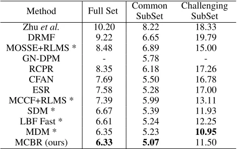
Table 1: The inter-pupil distance normalized landmark error (%) of the compared methods on the 300-W (Sagonas et al. 2013a) dataset.
Method Full Set Common
SubSet
Challenging SubSet Zhuet al. 10.20 8.22 18.33
DRMF 9.22 6.65 19.79
MOSSE+RLMS * 8.48 6.89 15.00
GN-DPM - 5.78
-RCPR 8.35 6.18 17.26
CFAN 7.69 5.50 16.78
ESR 7.58 5.28 17.00
MCCF+RLMS * 7.39 5.99 13.11
SDM * 6.67 5.39 11.93
LBF Fast * 6.61 5.24 12.25
MDM * 6.35 5.23 10.95
MCBR (ours) 6.33 5.07 11.50
68 annotated facial points for robustness evaluation of facial landmark detection algorithms. Following the same dataset configuration as in (Ren et al. 2014) , our training set con-sists of the training set of LFPW (Belhumeur et al. 2013) and Helen (Le et al. 2012), the whole AFW set (Zhu and Ramanan 2012), totally 3148 training images. Our test set consists of the test set of LFPW and Helen, and the whole IBUG set, totally 689 test images.
Implementation Details In this experiment, we conduct our proposed MCBR method atm= 3 different resolution layers, each layer containsn= 2 stages. The standard devi-ation in Equdevi-ation (6) to compute the BLDs is set to2. And the size of cropped patch is set to31×31. The number of iterations in L-BFGS is set to66.
To provide a better initial shape for an image, we di-vide the training set into three view-specific subsets, i.e., left
(−30◦,−0◦), frontal(−15◦,15◦)and right(0◦,30◦). The overlaps between adjacent views are considered for fault tol-erance. We decide which view range a face image belongs to by the distance between the pose of this image and the cen-tral poses of the three subsets, i.e.,−15◦,0◦,15◦ 1. Then,
we assign the mean shape of the corresponding view sub-sets as an initial shape for an image during the test phase. The average run time for our proposed MCBR method us-ing unoptimized Python implementations on an Intel Core i7 2.20-GHz machine is800ms per image with68landmarks. During training, we use data augmentation to enlarge the training data. For each training image, we randomly select the shape of other training images in the same view-specific subset as the initial shape four times. In this way, we gener-ate4perturbed initial shapes for each training image. During test, we only use the view-specific mean shape as the initial shape without multiple initializations. Note that we only use view-specific subsets to provide better initial shapes, rather than training our method separately in each view.
1
We apply the open source pose estimator to the 300-W dataset: https://github.com/mpatacchiola/deepgaze
Baselines We choose several existing state-of-the-art fa-cial landmark detection algorithms for comparison, includ-ing Zhu et al.(Zhu and Ramanan 2012), DMRF (Asthana et al. 2013), GN-DPM (Tzimiropoulos and Pantic 2014), RCPR (Burgos-Artizzu, Perona, and Doll´ar 2013), CFAN (Zhang et al. 2014), ESR (Cao et al. 2014), SDM (Xiong and De la Torre 2013), LBF Fast (Ren et al. 2014) and MDM (Trigeorgis et al. 2016). Also, we add two best CLM meth-ods, i.e., MOSSE+RLMS and MCCF+RLMS. The mean landmark errors (Ren et al. 2014) of different methods are reported in Table 1. The results of methods marked with * are obtained by our implementation, and others are directly obtained from the corresponding papers. It is worth noting that we only sample initial shapes for each training image 4 times to augment the training set, which is far less than the amount of training data for other trained models mentioned in their paper. MOSSE+RLMS, MCCF+RLMS, SDM and LBF Fast are all conducted in the Multi-scale Cascaded manner. The size of local patches in MOSSE/MCCF+RLMS is set to31×31. SDM uses the same HOG descriptors as ours. For LBF Fast, we set the number of trees at each stage to 68×6 = 408, and each tree depth is set to 5. The radiuses of two stages at each resolution layer are set to [0.3, 0.2], and the number of the randomly sampled candidate features in the local region is set to 500. For MDM, we set all param-eters the same as described in their paper. Bounding boxes provided by 300-W set are used for all implemented meth-ods. Initial shapes for the test images are set the same for all implemented methods.
Results We compare our method with the baseline meth-ods in Table 1. The MOSSE/MCCF+RLMS method per-forms worst in all implemented methods. MDM adopts the powerful CNN to learn the data-driven features and RNN to impose the memory constraint on the descent directions, so it performs better than LBF Fast and SDM on the Full Set. LBF Fast performs better than SDM, which benefits from its highly discriminative local binary features. While all baseline methods do not consider the issue of the inaccu-rate annotated landmarks, our method uses soft landmarks, i.e., BLD, to deal with the landmark noise, and thus achieve the best performance on the Full Set.
0 1 2 3 4 5 6 7 Variance of the inaccurate landmark noise 6
6.5 7 7.5 8 8.5 9
Mean Localization Error x 100
Robust results on the 300-W Full Set
MOSSE+RLMS MCCF+RLMS SDM LBF Fast MDM MCBR (OURS)
(a) Full Set
0 1 2 3 4 5 6 7 Variance of the inaccurate landmark noise 5
5.2 5.4 5.6 5.8 6 6.2 6.4 6.6 6.8 7
Mean Localization Error x 100
Robust results on the 300-W Common SubSet
MOSSE+RLMS MCCF+RLMS SDM LBF Fast MDM MCBR (OURS)
(b) Common Subset
0 1 2 3 4 5 6 7
Variance of the inaccurate landmark noise 10.5
11 11.5 12 12.5 13 13.5 14 14.5 15 15.5
Mean Localization Error x 100
Robust results on the 300-W Challenging SubSet
MOSSE+RLMS MCCF+RLMS SDM LBF Fast MDM MCBR (OURS)
(c) Challenging Subset
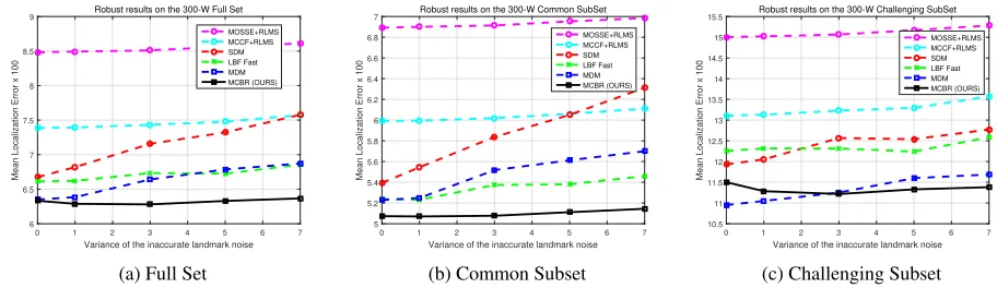
Figure 4: Results on the 300-W dataset (Sagonas et al. 2013a) when increasing the inaccurate annotated landmark noise.
Robustness against annotation noise
Our model appears robust against the increase of the in-accurate facial landmarks annotations since it associates a BLD for each landmark, which considers the neighboring pixels around the originally annotated landmark. To further demonstrate this, we design an experiment that gradually in-creases the annotated landmarks noise in the training set. In order to observe the performance of the algorithm, we keep the test set unchanged while the noise of the training land-marks gradually increases.
For the training images in the 300-W database, we im-pose annotation noise on the original landmarks. Annota-tion noise can be modeled as Gaussian distribuAnnota-tion ∼ N(;0,ρ2), which can be explained as the deviation pixel
distance from the original landmark.ρ2denotes the variance
of the noise, which reflects the inaccuracy of the annotated landmarks. In our experiments, we conduct 5 different vari-ances of the noise, i.e.,ρ2= [0, 1, 3, 5, 7]. We choose five compared methods from Table 1, the top three baseline al-gorithms, i.e., SDM (Xiong and De la Torre 2013), LBF Fast (Ren et al. 2014) and MDM (Trigeorgis et al. 2016), and two CLM method, i.e., MOSSE/MCCF+RLMS. The impletation details of all algorithms are set to the same as men-tioned above.
The performances of different algorithms against the in-crease of the landmark noise are shown in Fig. 4. Our model deals with facial landmark detection well not only in the value of the averaged landmark error, but also the robustness against more and more training annotated landmark noise. Generally speaking, for the Full Set in Fig. 4(a), although MOSSE/MCCF+RLMS does not seem to be sensitive to the landmark noise, their averaged landmark error is too high, which makes no sense. SDM deteriorates quickly with the increase of the inaccurate landmark noise. Compared with SDM, LBF Fast considers the shape constraints between the landmarks, the curve of it shows a relatively gentler ten-dency. Since MDM adopts effective convolutional features, it starts from a lower mean landmark error than LBF Fast. However, the data-driven MDM deteriorates faster than LBF Fast, revealing that the performance of MDM is sensitive to the landmark noise. Furthermore, our method deteriorates most slowly with the increase of the landmark noise.
For the Common Subset shown in Fig. 4(b), our method
shows the most slowest rising trend among all compared baselines against the increased landmark noise. For the Challenging SubSet shown in Fig. 4(c), since hand-crafted features are sub-optimal compared with convolutional fea-tures, our method starts from a higher position than MDM. However, with the increased landmark noise, our method gradually performs better than MDM. Note that there exist a phenomenon that some methods achieve a slightly better performance when increasing the landmark noise. For exam-ple, in Fig. 4(c), our method shows a slight improvement in the experiments of noise 1 than in noise 0. The reason might be that the performances in the Challenging Subset are sen-sitive to the initial shapes, and when increasing landmark noise, the initial shapes calculated from the training set for the test images also changed, which may cause experimental random improvements.
In summary, performance curves of our method on the different test subsets are rather stable than all compared baselines, which validates the robustness of our algorithm against the increased training landmark noise.
Conclusion and Future Work
Acknowledgments
This research was supported by the National Key Research & Development Plan of China (No. 2017YFB1002801), the National Science Foundation of China (61622203), the Jiangsu Natural Science Funds for Distinguished Young Scholar (BK20140022), the Collaborative Innovation Cen-ter of Novel Software Technology and Industrialization, and the Collaborative Innovation Center of Wireless Communi-cations Technology.
References
Asthana, A.; Zafeiriou, S.; Cheng, S.; and Pantic, M. 2013. Robust discriminative response map fitting with constrained local models. In Proceedings of the IEEE Conference on Computer Vision and Pattern Recognition, 3444–3451. Belhumeur, P. N.; Jacobs, D. W.; Kriegman, D. J.; and Ku-mar, N. 2013. Localizing parts of faces using a consensus of exemplars. IEEE transactions on pattern analysis and machine intelligence35(12):2930–2940.
Bolme, D. S.; Beveridge, J. R.; Draper, B. A.; and Lui, Y. M. 2010. Visual object tracking using adaptive correlation fil-ters. InComputer Vision and Pattern Recognition (CVPR), 2010 IEEE Conference on, 2544–2550. IEEE.
Burgos-Artizzu, X. P.; Perona, P.; and Doll´ar, P. 2013. Ro-bust face landmark estimation under occlusion. In Proceed-ings of the IEEE International Conference on Computer Vi-sion, 1513–1520.
Cao, X.; Wei, Y.; Wen, F.; and Sun, J. 2014. Face align-ment by explicit shape regression. International Journal of Computer Vision107(2):177–190.
Cootes, T. F.; Taylor, C. J.; Cooper, D. H.; and Graham, J. 1995. Active shape models-their training and application.
Computer vision and image understanding61(1):38–59. Cristinacce, D., and Cootes, T. 2008. Automatic feature localisation with constrained local models. Pattern Recog-nition41(10):3054–3067.
Galoogahi, H. K.; Sim, T.; and Lucey, S. 2013. Multi-channel correlation filters. InComputer Vision (ICCV), 2013 IEEE International Conference on, 3072–3079. IEEE. Geng, X., and Ling, M. 2017. Soft video parsing by label distribution learning. InAAAI, 1331–1337.
Geng, X.; Yin, C.; and Zhou, Z.-H. 2013. Facial age estima-tion by learning from label distribuestima-tions.IEEE Transactions on Pattern Analysis and Machine Intelligence35(10):2401– 2412.
Geng, X. 2016. Label distribution learning. IEEE Trans-actions on Knowledge and Data Engineering 28(7):1734– 1748.
Jesorsky, O.; Kirchberg, K. J.; and Frischholz, R. W. 2001. Robust face detection using the hausdorff distance. In Inter-national Conference on Audio-and Video-Based Biometric Person Authentication, 90–95. Springer.
Le, V.; Brandt, J.; Lin, Z.; Bourdev, L.; and Huang, T. S. 2012. Interactive facial feature localization. InEuropean Conference on Computer Vision, 679–692. Springer.
Liu, D. C., and Nocedal, J. 1989. On the limited mem-ory bfgs method for large scale optimization. Mathematical programming45(1):503–528.
Matthews, I., and Baker, S. 2004. Active appearance models revisited. International journal of computer vision
60(2):135–164.
Ren, S.; Cao, X.; Wei, Y.; and Sun, J. 2014. Face alignment at 3000 fps via regressing local binary features. In Proceed-ings of the IEEE Conference on Computer Vision and Pat-tern Recognition, 1685–1692.
Sagonas, C.; Tzimiropoulos, G.; Zafeiriou, S.; and Pantic, M. 2013a. 300 faces in-the-wild challenge: The first fa-cial landmark localization challenge. InProceedings of the IEEE International Conference on Computer Vision Work-shops, 397–403.
Sagonas, C.; Tzimiropoulos, G.; Zafeiriou, S.; and Pantic, M. 2013b. A semi-automatic methodology for facial land-mark annotation. InProceedings of the IEEE Conference on Computer Vision and Pattern Recognition Workshops, 896– 903.
Saragih, J. M.; Lucey, S.; and Cohn, J. F. 2011. Deformable model fitting by regularized landmark mean-shift. Interna-tional Journal of Computer Vision91(2):200–215.
Trigeorgis, G.; Snape, P.; Nicolaou, M. A.; Antonakos, E.; and Zafeiriou, S. 2016. Mnemonic descent method: A re-current process applied for end-to-end face alignment. In
Proceedings of the IEEE Conference on Computer Vision and Pattern Recognition, 4177–4187.
Tsoumakas, G., and Katakis, I. 2006. Multi-label classifica-tion: An overview.International Journal of Data Warehous-ing and MinWarehous-ing3(3).
Tzimiropoulos, G., and Pantic, M. 2014. Gauss-newton de-formable part models for face alignment in-the-wild. In Pro-ceedings of the IEEE Conference on Computer Vision and Pattern Recognition, 1851–1858.
Xiong, X., and De la Torre, F. 2013. Supervised descent method and its applications to face alignment. In Proceed-ings of the IEEE conference on computer vision and pattern recognition, 532–539.
Zhang, J.; Shan, S.; Kan, M.; and Chen, X. 2014. Coarse-to-fine auto-encoder networks (cfan) for real-time face align-ment. InEuropean Conference on Computer Vision, 1–16. Springer.
Zhao, W.; Chellappa, R.; Phillips, P. J.; and Rosenfeld, A. 2003. Face recognition: A literature survey.ACM computing surveys (CSUR)35(4):399–458.
Zhou, Y.; Xue, H.; and Geng, X. 2015. Emotion distribution recognition from facial expressions. InProceedings of the 23rd ACM international conference on Multimedia, 1247– 1250. ACM.