Confidence Sets with Expected Sizes
for Multiclass Classification
Christophe Denis [email protected]
LAMA UMR-CNRS 8050
Universit´e Paris-Est Marne-la-Vall´ee
5 Bd Descartes, 77454 Marne-la-Vall´ee cedex 2, France
Mohamed Hebiri [email protected]
LAMA UMR-CNRS 8050
Universit´e Paris-Est Marne-la-Vall´ee
5 Bd Descartes, 77454 Marne-la-Vall´ee cedex 2, France
Editor:G´abor Lugosi
Abstract
Multiclass classification problems such as image annotation can involve a large number of classes. In this context, confusion between classes can occur, and single label classification may be misleading. We provide in the present paper a general device that, given an unla-beled dataset and a score function defined as the minimizer of some empirical and convex risk, outputs a set of class labels, instead of a single one. Interestingly, this procedure does not require that the unlabeled dataset explores the whole classes. Even more, the method is calibrated to control the expected size of the output set while minimizing the classification risk. We show the statistical optimality of the procedure and establish rates of convergence under the Tsybakov margin condition. It turns out that these rates are linear on the number of labels. We apply our methodology to convex aggregation of confidence sets based on theV-fold cross validation principle also known as the superlearning princi-ple (van der Laan et al., 2007). We illustrate the numerical performance of the procedure on real data and demonstrate in particular that with moderate expected size, w.r.t. the number of labels, the procedure provides significant improvement of the classification risk.
Keywords: Multiclass Classification, Confidence Sets, Empirical Risk Minimization, Convex Loss, Superlearning
1. Introduction
The advent of high-throughput technology has generated tremendous amounts of large and high-dimensional classification data. This allows classification at unprecedented scales with hundreds or even more classes. The standard approach to classification in the multiclass setting is to use a classification rule for assigning a single label. More specifically, it consists in assigning a single label Y ∈ Y, with Y ={1, . . . , K}, to a given input example X ∈ X
among a collection of labels. However, while a large number of classes can lead to precise characterizations of data points, similarities among classes also bear the risk of confusion and misclassification. Hence, assigning a single label can lead to wrong or ambiguous results. In this paper, we address this problem by introducing an approach that yields sets of labels as outputs, namely, confidence sets. A confidence set Γ is a function that maps X
c
onto 2Y. A natural way to obtain a set of labels is to use ranked outputs of the classification rule. For example, one could take the classes that correspond to the top-level conditional probabilities P(Y =·|X=x). Here, we provide a more general approach where we control
the expected size of the confidence sets. For a confidence set Γ, the expected size of Γ is defined as E[|Γ(X)|], where | · | stands for the cardinality. For a sample X and given an
expected set sizeβ, we provide an algorithm that outputs a set ˆΓ(X) such thatE[|Γ(ˆ X)|]≈
β. Furthermore, the procedure aims at minimizing the classification error given by
P
Y /∈Γ(ˆ X)≈ min
Γ :E[|Γ(X)|]=βP(Y /
∈Γ(X)) =R∗β.
We establish a close formula of the oracle confidence set Γ∗ = argminΓ :E[|Γ(X)|]=βP(Y /∈Γ(X))
that involves the cumulative distribution functions of the conditional probabilities. Besides, we formulate a data-driven counterpart of Γ∗ based on the minimization of the empirical risk. However, the natural risk function in the multiclass setting is non convex, and then minimizing it is proving to be a computational issue. As a remedy, convex surrogates are often used in machine learning, and more specifically in classification as reflected by the popularity of methods such as Boosting (Freund and Schapire, 1997), logistic regres-sion (Friedman et al., 2000) and support vector machine (Vapnik, 1998). In our problem this translates by considering some convex surrogate of the 0/1-loss in P(Y /∈Γ(X)); we
introduce a new convex risk function which enables us to emphasize specific aspects of con-fidence sets. That convex risk function is partly inspired by the works by Zhang (2004), Bartlett et al. (2006) and Yuan and Wegkamp (2010), that deal with binary classification.
Our approach displays two main features. First, our method can be implemented in a semi-supervised way (Vapnik, 1998). More precisely, the method is a two-steps procedure that requires the estimation of score functions (as minimizers of some convex risk function) in a first step and the estimation of the cumulative distribution of these scores in a sec-ond one. Hence, the first step requires labeled data whereas the secsec-ond one involves only unlabeled samples. Notably, the unlabeled sample does not necessary consists of examples coming from the whole classes. This aspects is fondamental when we deal with a large num-ber of classes, some of which been sparsely represented. Second, from the theoretical point of view, we provide an oracle inequality satisfied by ˆΓ, the empirical confidence set that results from the minimization of an empirical convex risk. The obtained oracle inequality shall enable us to derive rates of convergence on a particular class of confidence sets under the Tsybakov noise assumption on the data generating distribution. These rates are linear in the number of classesK and also depend on the regularity of the cumulative distribution functions of the conditional probabilities.
for-est procedures or softmax regression since these methods are popular in machine learning and that each of them is associated to a different shape.
We end up this discussion by highlighting in two words what we perceive as being the main contributions of the present paper. We describe an optimal strategy for building con-fidence sets in multiclass classification setting, and we derive a new aggregation procedure for confidence sets that still allows controlling the expected size of the resulting confidence set.
Related works: The closest learning task to the present work is classification with reject option which is a particular setting in binary classification. Several papers fall within the scope of this area (Chow, 1970; Herbei and Wegkamp, 2006; Yuan and Wegkamp, 2010; Wegkamp and Yuan, 2011; Lei, 2014; Denis and Hebiri, 2015) and differ from each other by the goal they consider. Among these references, our procedure is partially inspired by Denis and Hebiri (2015) that also consider a semi-supervised approach to build confidence sets invoking some cumulative distribution functions (of the conditional probabilities themselves in their case). The similarity is however limited to the definition of oracle confidence sets, the oracle confidence in the present paper being an extension of the one defined in the paper by Denis and Hebiri (2015) to the multiclass setting. On the other hand, all the data-driven considerations are completely different (in particular, Denis and Hebiri (2015) focus on plug-in rules) and importantly, we develop here new probabilistic results on sums of cumulative distribution functions of random variables, that are of own interest.
Assigning a set of labels instead of a single one for an input example is not new (Vovk et al., 2005; Wu et al., 2004; del Coz et al., 2009; Lei et al., 2013; Choromanska et al., 2016). One of the most popular methods is based onConformal Prediction approach (Vovk et al., 1999; Vovk, 2002; Vovk et al., 2005). In the multiclass classification framework, the goal of this algorithm is to build the smallest set of labels such that its classification error is below a pre-specified level. Since our procedure aims at minimizing the classification error while keeping under control the size of the set, Conformal Prediction can be seen as a dual of our method. It is worth mentioning that conformal predictors approaches need two labeled datasets where we only need one labeled dataset, the second being unlabeled. We refer to the very interesting statistical study of Conformal Predictors in the binary case in the paper by Lei (2014).
Notation: First, we state general notation. Let Y = {1, . . . , K}, with K ≥ 2 being an integer. Let (X, Y) be the generic data-structure taking its values inX ×Ywith distribution
P. The goal in classification is to predict the label Y given an observation of X. This is
performed based on a classifier (or classification rule)swhich is a function mappingX onto
Y. Let S be the set of all classifiers. The misclassification risk R associated with s∈ S is defined as
R(s) =P(s(X)6=Y).
Moreover, the minimizer of R over S is the Bayes classifier, denoted by s∗, and is charac-terized by
s∗(·) = argmax
k∈Y
pk(·),
wherepk(x) =P(Y =k|X=x) for x∈ X and k∈ Y.
Let a confidence set be any measurable function that mapsX onto 2Y. Let Γ be a confidence set. This confidence set is characterized by two attributes. The first one is the risk associated to the confidence set
R(Γ) =P(Y /∈Γ(X)), (1)
and is related to its accuracy. The second attribute is linked to the information given by the confidence set. It is defined as
I(Γ) =E(|Γ(X)|), (2)
where | · | stands for the cardinality. Moreover, for some β ∈ [1, K], we say that, for two confidence sets Γ and Γ0 such thatI(Γ) =I(Γ0) =β, the confidence set Γ is “better” than Γ0 ifR(Γ)≤ R(Γ0).
Organization of the paper: The rest of the paper is organized as follows. Next section is devoted to the definition and the main properties of the oracle confidence set for multiclass classification. The empirical risk minimization procedure is provided in Section 3. Rates of convergence for the confidence set that results from this minimization can also be found in this section. We present an application of our procedure to aggregation of confidence sets in Section 4. We finally draw some conclusions and present perspectives of our work in Section 5. Proofs of our results are postponed to the Appendix.
2. Confidence set for multiclass classification
In the present section, we define a class of confidence sets that are suitable for multiclass classification and referred asOracleβ-sets. For someβ ∈(0, K), these sets are shown to be optimal according to the risk (1) with an information (2) equal to β. Moreover, basic but fondamental properties of Oracleβ-sets can be found in Proposition 1, while Proposition 7 provides another interpretation of these sets.
2.1 Notation and definition
First of all, we introduce in this section a class of confidence sets that specifies oracle confidence sets. Let β ∈(0, K) be a desired information level. The so-calledOracle β-sets
are optimal according to the risk (1) among all the confidence sets Γ such that I(Γ) =β. Throughout the paper we make the following assumption
(A1) For all k∈ {1, . . . , K}, the cumulative distribution function Fpk of pk(X) is
continu-ous.
The definition of the Oracle β-set relies on the continuous and decreasing function G defined for anyt∈[0,1] by
G(t) =
K
X
k=1
¯ Fpk(t),
where for any k ∈ {1, . . . , K}, we denote by ¯Fpk the tail distribution function of pk(X),
that is, ¯Fpk = 1−Fpk withFpk being the cumulative distribution function (c.d.f.) ofpk(X).
The generalized inverseG−1 ofG is given by (see (van der Vaart, 1998)):
The functions G and G−1 are central in the construction of the Oracle β-sets. We then provide some of their useful properties in the following proposition.
Proposition 1 The following properties on G hold
i) For every t∈(0,1) and β∈(0, K), G−1(β)≤t⇔β≥G(t).
ii) For every β∈(0, K), G(G−1(β)) =β.
iii) Let εbe a random variable, independent of X, and distributed from a uniform distri-bution on {1, . . . , K} and let U be uniformly distributed on [0, K]. Define
Z =
K
X
k=1
pk(X)1{ε=k}.
If the function Gis continuous, then G(Z)=L U and G−1(U)=L Z.
The proof of Proposition 1 relies on Lemma 1 in the Appendix. Now, we are able to defined the Oracleβ-set:
Definition 2 Let β∈(0, K), the Oracle β-set is given by
Γ∗β(X) = {k∈ {1, . . . , K}: G(pk(X))≤β}
= k∈ {1, . . . , K}: pk(X)≥G−1(β) .
This definition of the Oracleβ-set is intuitive and can be related to the binary classification with reject option setting (Chow, 1970; Herbei and Wegkamp, 2006; Denis and Hebiri, 2015) in the following way: a label k is assigned to the Oracle β-set if the probability pk(X) is
large enough. It is worth noting that the function G plays the same role as the c.d.f. of the score function used by Denis and Hebiri (2015). As emphasized by Proposition 1, their introduction allows to control exactly the information (2). Indeed, it follows from the definition of the Oracleβ-set that for eachβ ∈(0, K)
|Γ∗β(X)|=
K
X
k=1
1{pk(X)≥G−1(β)},
and thenI(Γ∗β) =E
h
|Γ∗β(X)|i=G(G−1(β)). Therefore, Proposition 1 ensures that
I(Γ∗β) =β.
This last display points out that the Oracleβ-sets are indeedβ-level (that is, its information equals β). In the next section, we focus on the study of the risk of these oracle confidence sets.
2.2 Properties of the oracle confidence sets
Let us first state the optimality of the Oracleβ-set:
Proposition 4 Let Assumption (A1) be satisfied. For any β ∈(0, K), we have both:
1. The Oracle β-setΓ∗β satisfies the following property:
R Γ∗β
= inf
Γ R(Γ), where the infimum is taken over all β-level confidence sets.
2. For any β-level confidence set Γ, the following holds
0≤ R(Γ)− R Γ∗β=E
X
k∈(Γ∗
β(X) ∆ Γ(X))
pk(X)−G−1(β)
, (3)
where the symbol ∆ stands for the symmetric difference of two sets, that is, for two subsets A and B of {1, . . . , K}, we write A∆B = (A\B)∪(B\A).
Several remarks can be made from Proposition 4. First, for β ∈ (0, K), the Oracle β-set is optimal for the misclassification risk, over the class of β-level confidence sets. Moreover, the excess risk of any β-level confidence set relies on the behavior of the score functions pk around the threshold G−1(β). Finally, we can note that if K = 2 and β = 1, which
implies that G−1(β) = 1/2, Equation (3) reduces to the misclassification excess risk in binary classification.
Remark 5 One way to build a confidence setΓ with informationβ is to setΓas theβ top levels conditional probabilities. In the sequel this method is referred as the max procedure. This strategy is natural but actually suboptimal as shown by the first point of Proposition 4. As an illustration, we consider a simulation scheme with K = 10 classes. We generate
(X, Y) according to a mixture model. More precisely,
i) the label Y is distributed from a uniform distribution on {1, . . . , K};
ii) conditional onY =k, the feature X is generated according to a multivariate gaussian distribution with mean parameter µk∈R10 and identity covariance matrix. For each
k= 1, . . . , K, the vectors µk are i.i.d realizations of uniform distribution on [0,4].
For β = 2 we evaluate the risks of the Oracle β-set and the max procedure and obtain respectively 0.05 and 0.09 (with very small variance).
Remark 6 An important motivation behind the introduction of confidence sets and in par-ticular of Oracle β-sets is that they might outperform the Bayes rule which can be seen as the Oracleβ-set associated toβ = 1. This gap in performance is even larger when the num-ber of classes K is large and there is a big confusion between classes. Such improvement will be illustrated in the numerical study (see Section 4.3).
Proposition 7 For t∈[0,1], andΓ a confidence set, we define
Lt(Γ) =P(Y /∈Γ(X)) +tI(Γ).
For β∈[0, K], the following equality holds:
LG−1(β)(Γ∗β) = min
Γ LG
−1(β)(Γ).
The proof of this proposition relies on the same arguments as those of Proposition 4. It is then omitted. Proposition 7 states that the Oracle β-set is defined as the minimizer, over all confidence sets Γ, of the risk function Lt when the tuning parameter t is set equal to
G−1(β). Note moreover that the risk functionLtis a trade-off, controlled by the parameter
t, between the risk of a confidence set on the one hand, and the information provided by this confidence set on the other hand. Hence, the risk function Lt can be viewed as
a generalization to the multiclass case of the risk function provided by Chow (1970) and Herbei and Wegkamp (2006) for binary classification with reject option setting.
3. Empirical risk minimization
In this section we introduce and study confidence sets which rely on the minimization of convex risks. Their definitions and main properties are given in Sections 3.1-3.2. As a consequence, we deduce a data-driven procedure described in Section 3.3 with several theoretical properties, such as rates of convergence, that we demonstrate in Section 3.4.
3.1 φ-risk
Let f = (f1, . . . , fK) : X → RK be a score function and Gf(.) = PKk=1F¯fk(.). Assuming
that the function Gf is continuous and given an information level β ∈(0, K), there exists
δ∈R, such thatGf(−δ) =β. Given this simple but important fact, we define the confidence
set Γf,δ associated to f and δ as
Γf,δ(X) ={k : fk(X)≥ −δ}. (4)
In this way, the confidence set Γf,δ consists of top scores, and the threshold δ is fixed so
thatI(Γf,δ) =β. As a consequence, we naturally aim at solving the problem
min
f∈FR(Γf,δ),
where F is a class of functions. Due to computational issues, it is convenient to focus on a convex surrogate of the previous minimization problem. To this end, let φ:R→Rbe a
convex function. We define the φ-risk of f by
Rφ(f) =E
" K X
k=1
φ(Zkfk(X))
#
, (5)
whereZk = 21{Y=k}−1 for allk= 1, . . . , K. Therefore, our target score becomes
¯
f ∈argmin
f∈F
for the purpose of building the confidence Γf ,δ¯ . In the sequel, we also introduce f∗, the
minimizer over the class of all measurable functions, of theφ-risk. The notation suppresses the dependence on φ. It is worth mentioning at this point that the definition of the risk functionRφis dictated by Equation (3) and suits for confidence sets. Moreover, this
func-tion differs from the classical risk funcfunc-tion used in the multiclass setting (see (Tewari and Bartlett, 2007)). The reason behind this is that building a confidence set is closer to K binary classification problems.
3.2 Classification calibration for confidence sets
Convexification of the risk in classification is a standard technique. In this section we adapt classical results and tools to confidence sets in the multiclass setting. We refer the reader to earlier papers for interesting developments (Zhang, 2004; Bartlett et al., 2006; Yuan and Wegkamp, 2010).
One of the main important concept when we deal with convexification of the risk is the notion of calibration of the loss function φ. This property permits to connect confidence sets deduced from the convex risk and from the classification risk.
Definition 8 We say that the function φ is confidence set calibrated if for allβ >0, there exists δ∗∈Rsuch that
Γf∗,δ∗= Γ∗β,
with f∗ being the minimizer of the φ-risk
f∗ ∈argmin
f
Rφ(f),
where the infimum is taken over the class of all measurable functions. Hence, the confidence set based on f∗ coincides with the Bayes confidence set.
Given this, we can state the following proposition that gives a characterization of the con-fidence set calibration property in terms of the functionG.
Proposition 9 The functionφis confidence set calibrated if and only if for all β∈(0, K), there exists δ∗ ∈Rsuch that φ0(δ∗) and φ0(−δ∗) both exists, φ0(δ∗)<0, φ0(−δ∗)<0 and
G−1(β) = φ
0(δ∗)
φ0(δ∗) +φ0(−δ∗) ,
where φ0 denotes the derivative ofφ.
et al., 2006; Wegkamp and Yuan, 2011)). Now, for some score function f and some real number δ such thatGf(−δ) =β, we define the excess risk
∆R(Γf,δ) =R(Γf,δ)− R(Γ∗β),
and the excess φ-risk
∆Rφ(f) =Rφ(f)−Rφ(f∗).
We also introduce the marginal conditional excess φ-risk on f = (f1, . . . , fK) as
∆Rkφ(f(X)) =pk(X)(φ(fk(X))−φ(fk∗(X))) + (1−pk(X))(φ(−fk(X))−φ(−fk∗(X))),
for k = 1, . . . , K. The following theorem shows that the consistency in terms of φ-risk implies the consistency in terms of classification riskR.
Theorem 10 Assume thatφ is confidence set calibrated and assume that there exists con-stants C >0 and s≥1 such that1
|pk(X)−G−1(β)|s≤C∆Rkφ(−δ
∗
). (6)
Let fˆn be a sequence of scores. We assume that for each n, the functionGfnˆ is continuous. Let δn∈R be such thatGfnˆ (−δn) =β, then
∆Rφ( ˆfn) P
→0 ⇒ ∆R(Γfn,δnˆ )
P
→0.
The theorem ensures that the convergence in terms of φ risk implies the convergence in terms of riskR. This convergence is made possible since we manage, in the proof, to bound the excess risk by (a power of) the excessφ-risk. The assumption needed in this theorem is also standard and is for instance satisfied for the boosting, least square and logistic losses with the parameter sbeing equal to 2 (see (Bartlett et al., 2006)).
3.3 Data-driven procedure
In this section we provide the steps of the construction of our empirical confidence set that is deduced from the empirical risk minimization. Before going into further details, let us first mention that our procedure is semi-supervised in the sense that it requires two datasets, one of which being unlabeled. Hence we introduce a first data setDn={(Xi, Yi), i= 1, . . . , n},
which consists of independent copies of (X, Y). We define the empirical φ-risk associated to a score function f (which is the empirical counterpart ofRφgiven in (5)):
ˆ Rφ(f) =
1 n
n
X
i=1
K
X
k=1
φ(Zkifk(Xi)), (7)
whereZi
k= 21{Yi=k}−1 for all k= 1, . . . , K. We also define the empirical risk minimizer
overF, a convex set of score functions, as
ˆ
f = arg min
f∈F
ˆ Rφ(f).
1. With abuse of notation, we write ∆Rkφ(−δ
∗
) instead of ∆Rkφ((−δ
∗
At this point, we have in hands the optimal score function ˆf and need to build the corre-sponding confidence set with the right expected size. However, let us before introduce an intermediate confidence set that would help comprehension since it mimics the oracleβ-set Γ∗ with regard to its construction using ˆf instead off∗. For this purpose, we define
Ffkˆ(t) =PX
ˆ
fk(X)≤t|Dn
,
for t∈ R, wherePX is the marginal distribution of X. As for the c.d.f. ofpk and fk, we
make the following assumption:
(A2) The cumulative distribution functionsFfˆ
k withk= 1, . . . , K are continuous.
At this point, we are able to define an empirical approximation of the Oracle β-set for β ∈(0, K):
e
Γβ(X) =
n
k∈ {1, . . . , K}: Ge( ˆfk(X))≤β o
, (8)
where fort∈R
e
G(t) =
K
X
k=1
¯
Ffkˆ(t), (9)
with ¯Ffkˆ = 1−Ffkˆ. Since the function Ge depends on the unknown distribution of X, we
consider a second but interestinglyunlabeleddatasetDN ={Xi, i= 1, . . . , N}, independent
of Dn in order to compute the empirical versions of the ¯Ffˆ
k’s. By now, we can define the
empiricalβ-set based on ˆf:
Definition 11 Let fˆbe the minimizer of the empirical φ-risk given in (7) based on Dn,
and consider the unlabeled datasetDN. Let β ∈(0, K). The empirical β-set is given by
ˆ
Γβ(X) =
n
k∈ {1, . . . , K}: ˆG( ˆfk(X))≤β
o
, (10)
where
ˆ
G(.) = 1 N
N
X
i=1
K
X
k=1
1{fkˆ(Xi)≥.}.
The most important remark about the construction of this data-driven confidence set is that it is made in a semi-supervised way. Indeed, the estimation of the tail distribution functions of ˆfk requires only a set ofunlabeled observations. This is particularly attractive
in applications where the number of label observations is small (because labelling examples is time consuming or may be costly) and where one has in hand several unlabeled features that can be used to make prediction more accurate. As an important consequence is that the estimation of the tail distribution functions of ˆfk does not depend on the number of
3.4 Rates of convergence
In this Section, we provide rates of convergence for the empirical confidence sets defined in Section 3.3. First, we state some additional notation. In the sequel, the symbols P
and E stand for generic probability and expectation, respectively. Moreover, given the empiricalβ-set ˆΓβ from Definition 11, we consider the risk R
ˆ Γβ
=PY /∈Γˆβ(X)
and
the information IΓˆβ
=Eh|Γˆβ(X)|
i
. Our first result ensures that ˆΓβ is of level β up to
a term of orderK/√N.
Proposition 12 For each β ∈(0, K), the following equality holds
I
ˆ Γβ
=β+O
K
√
N
.
In order to precise rates of convergence for the risk, we need to formulate several assump-tions. First, we consider loss functions φ which have in common that the modulus of convexity of their underlying risk function Rφ, defined by
δ(ε) = inf
(
Rφ(f) +Rφ(g)
2 −Rφ
f +g 2
,
K
X
k=1
EX(fk−gk)2(X)
≥ε2
)
, (11)
satisfies δ(ε) ≥ c12 for some c1 > 0 (we refer to (Bartlett et al., 2006; Bartlett and
Mendelson, 2006) for more details on modulus of convexity for classification risk). Moreover, we assume thatφis classification calibrated and L-Lipschitz forL >0. On the other hand, forα >0, we assume a margin condition Mkα on eachpk, k= 1, . . . , K (Tsybakov, 2004).
Mkα: PX 0<|pk(X)−G−1(β)| ≤t
≤c2tα, for some constant c2>0 and for all t >0.
It is important to note that since we assume that the distribution functions of pk(X) are
continuous for each k, we havePX 0<|pk(X)−G−1(β)| ≤t
→0 witht→0. Therefore, the margin condition only precise the rate of this decay to 0. Now, we provide the rate of convergence that we can expect for the empirical confidence sets defined by Equation (10).
Theorem 13 Assume that kfk∞ ≤ B for all f ∈ F. Let Mn = N(1/n, L∞,F) be the cardinality of the set of closed balls with radius 1/n inL∞-norm needed to cover F. Under the assumptions of Theorem 10, with the modulos of convexity δ(ε)≥c12 with c1>0, ifφ is L-Lipschitz and if the margin assumptions Mkα are satisfied withα >0, then
E h
|∆R(ˆΓβ)|
i
≤C(B, L, s, α)K1−α/(α+s)
inf
f∈F∆Rφ(f) +
Klog(Mn)
n
α/(α+s)
+C0√K
N,
where C0 >0 is an absolute constant and C(B, L, s, α)>0 is a constant that depends only onL, B, s and α.
From this theorem we obtain the following rate of convergence: Klog(nMn)α/(α+s)+ √K
N.
this rate is linear in K, the number of classes, that seems to be the characteristic of multiclass classification as compared to binary classification. Note that the exponent α/(α+s) is not classical and is due to the estimation of quantiles. The second part of the rates which is of order K/√N relies on the estimation of the function ˜G given in (9). This part of the estimation is established under the mild Assumptions (A1) and (A2). For this term the proof of the linearity onK is tricky and is obtained thanks to a new technical probabilistic results on sums of cumulative distribution functions (see Lemma 1). Let us conclude this paragraph by mentioning that Theorem 13 applies for instance forF being the convex hull of a finite family of a score functions which is the scope of the next section.
4. Application to confidence sets aggregation
This Section is devoted to an aggregation procedure which relies on the superlearning prin-ciple. The specifics of our superlearning procedure is given in Section 4.1. In Section 4.2, we show the consistency of our procedure and finally we provide a numerical illustration in Section 4.3 of our algorithm.
4.1 Description of the procedure: superlearning
In this section, we describe the superlearning procedure for confidence sets. The superlearn-ing procedure is based on the V-fold cross-validation procedure (see (van der Laan et al., 2007)). Initially, this aggregation procedure has been introduced in the context of regression and binary classification. LetV ≥2 be an integer and let (Bv)1≤v≤V be a regular partition of
{1, . . . , n},i.e., a partition such that, for eachv= 1, . . . , V, card(Bv)∈ {bn/Vc,bn/Vc+1},
where we write bxc for the floor of any real number x (that is, x−1≤ bxc ≤x). For each v ∈ {1, . . . , V}, we denote by D(nv) (respectively D
(−v)
n ) the dataset {(Xi, Yi), i ∈Bv}
(re-spectively {(Xi, Yi), i6∈Bv}), and define the corresponding empirical measures
Pn(v) = 1 card(Bv)
X
i∈Bv
Dirac(Xi, Yi), and
Pn(−v) = 1
n−card(Bv)
X
i6∈Bv
Dirac(Xi, Yi).
For a score algorithmf, that is to say a function which maps the empirical distribution to a score function. We define the cross-validated risk of f as
b
Rnφ(f) = 1 V
V
X
v=1
R(P (v)
n ) φ
f(Pn(−v)), (12)
where for eachv∈ {1, . . . , V},R(P (v)
n ) φ (f(P
(−v)
n )) is the empirical estimator ofRφ(f(P
(−v)
n ),
based onD(nv) and conditionally onD(−n v):
R(P (v)
n ) φ
f(Pn(−v))= 1 card(Bv)
X
i∈Iv K
X
k=1
Next, we considerF = f1, . . . , fM
a family of M score algorithms. We define the cross-validated score by
b
f ∈ argmin
f∈conv(F) b
Rφn(f). (13)
Finally, we consider the resulting cross-validated confidence set defined by
ˆ
ΓCVβ (X) =nk∈ {1, . . . , K}: ˆG( ˆfk(X))≤β
o
,
that we analyse in the next section.
4.2 Consistency of the algorithm
In this Section, we show some results that illustrate the consistency of the superlearning procedure described above. To this end, we introduce the oracle counterpart of the cross-validated risk defined in (12). For a scoref, we define
˜
Rnφ(f) = 1 V
V
X
v=1
Rφ(f(Pn(−v)),
that yields to the oracle counterpart of the cross-validated score defined in (13)
˜
f ∈ argmin
f∈conv(F)
˜ Rφn(f).
Here again, we assume that the loss function φ satisfies the properties described in Sec-tion 3.4 so that we can state the following result:
Proposition 14 We assume that for each f ∈ conv(F) and v ∈ {1, . . . , V} we have kf(Pn(−v))k∞≤B. Then the following holds
EhR˜nφ( ˆf)−R˜φn( ˜f)i≤C(B, L)KMlog(n)
bn/Vc ,
where C(B, L)>0 is a constant that depends only on B and L.
As usual when one deals with cross-validated estimators, the theorem compares ˆf to the oracle counterpart ˜f in terms of the oracle cross-validatedφ-risk. The theorem teaches us that, for sufficiently large n, ˆf perform as well as ˜f. However our main goal remains con-fidence sets. Therefore the next step consists in showing that the concon-fidence set associated to the cross-validated score ˆf has good properties in terms of the classification risk. Let Γf,δ be the confidence set that results from a choice of β ∈ (0, K) and a score function
f ∈conv(F). We introduce the following excess risks
∆ ˜Rn(Γf,δ) =
1 V
V
X
v=1 R
Γ
f
Pn(−v)
,δ
− R∗,
∆ ˜Rnφ(f) = 1 V
V
X
v=1
Rφ(f(Pn(−v)))−Rφ(f∗).
Forest(K= 4)
β-set
β rforest softmax reg svm kknn CV
2 R 0.02 (0.02) 0.06 (0.02) 0.02 (0.01) 0.05 (0.03) 0.02 (0.01)
I 2.00 (0.09) 2.00 (0.08) 2.00 (0.09) 2.00 (0.08) 2.00 (0.08)
Plant(K= 100)
β-set
β rforest softmax reg svm kknn CV
2 R 0.18 (0.03) 0.77 (0.02) 0.32 (0.04) 0.20 (0.03) 0.17 (0.03)
I 2.00 (0.09) 2.02 (0.18) 1.99 (0.10) 2.00 (0.08) 2.00 (0.08) 10 R 0.02 (0.01) 0.42 (0.04) 0.03 (0.02) 0.08 (0.03) 0.02 (0.01)
I 9.95 (0.38) 10.06 (0.58) 9.98 (0.22) 9.98 (0.23) 9.96 (0.37)
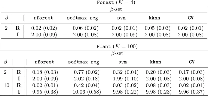
Table 1: For each of theB = 100 repetitions and for each dataset, we derive the estimated risks Rand informationI of the differentβ-sets w.r.t. β. We compute the means and standard deviations (between parentheses) over theB = 100 repetitions. For eachβ, theβ-sets are based on, from left to right,rforest,softmax regandsvm,
kknn and CV which are respectively the random forest, the softmax regression, support vector machines, k nearest neighbors and the superlearning procedure. Top: the dataset is the Forest– the dataset is thePlant.
Proposition 15 We assume that for eachv ∈ {1, . . . , V}, t7→PXfˆPn(−v)
≤t|Dn is
continuous. Under the assumptions of Proposition 14 and if the margin assumptions Mkα
are satisfied with α >0,
E h
|∆ ˜Rn(ˆΓCVβ )|i≤C(B, L, α, s)K1−α/(α+s)
E
h
∆ ˜Rnφ( ˜f)
i
+KMlog(n)
bn/Vc
α/(α+s)
+C0√K
N.
The proof of Proposition 15 relies on Proposition 14 and similar arguments as in Theorem 13.
4.3 Application to real datasets
In this section, we provide an application of our aggregation procedure described in Sec-tion 4.1. For the numerical experiment we focus on the boosting loss and consider the library of algorithms constituted by the random forest, the softmax regression, the support vector machines and the k nearest neighbors (with k= 11) procedures. To be more specifics, we respectively exploit the R packages randomForest, polspline, e1071 and kknn. All the
R functions are used with standard tuning parameters. Finally the parameter V of the aggregation procedure is fixed to 5.
We evaluate the performance of the procedure on two real datasets: the Forest type mapping dataset and the one-hundred plant species leaves dataset coming from the UCI database. In the sequel we refer to these two datasets as Forest and Plant respectively. The Forest dataset consists of K = 4 classes and 523 labeled observations (we gather the train and test sets) with 27 features. Here the classes are unbalanced. In the Plant
so that each class consists of 16 observations. The original dataset contains 3 covariates (each covariate consists of 64 features). In order to make the problem more challenging, we drop 2 covariates.
To get an indication of the statistical significance, it makes sense to compare our aggre-gated confidence set (referred asCV) to the confidence sets that result from each component of the library. Roughly speaking, we evaluate risks (and informations) of these confidence sets on each dataset. To do so, we use thecross validation principle. In particular, we run B = 100 times the procedure where we split the data each time in three: a sample of sizen to build the scores ˆf; a sample of sizeN to estimate the functionGand to get the confidence sets; and a sample of size M to evaluate the risk and the information. For both datasets, we make sure that in the sample of sizen, there is the same number of observations in each class. As a benchmark, we notify that the misclassification risks of the best classifier from the library in the Forestdataset is evaluated at 0.15 , whereas in the Plantdataset, it is evaluated at 0.40. As planned, the performance of the classical methods are quite bad in this last dataset.
We set the sizes of the samples as n = 200, N = 100 and M = 223 for the Forest
dataset, and n= 1000,N = 200 andM = 400 for the Plantone. The results are reported in Table 1, and confirm our expectations. In particular, our main observation is that the aggregated confidence set (CV) outperforms all components of the library in the sense that it is at least as good as the best component in all of the experiments. Second, let us state some remarks that hold for all of the confidence sets and in particular our aggregated confidence set. First, we note that the informationI(Γ) has the good levelβ which is supported by our theory. Moreover, we see that the risk gets drastically better with moderateβ as compared to thebestmisclassification risk. For instance, for thePlant, the error rate of the confidence set with β = 2 based on random forests is 0.18 whereas the misclassification error rate of the best component is 0.40.
5. Conclusion
This section gathers the proofs of our results. Let us first add a notation that will be used throughout the Appendix: for any random variable (or vector) Z, we denote by PZ
the probability w.r.t. Z and by EZ, the corresponding expectation.
Appendix A. Technical Lemmas
We first lay out key lemmata, which are crucial to establish the main theory. We consider K ≥2 be an integer, andZ1, . . . , ZK,K random variables. Moreover we define functionH
by:
H(t) = 1 K
K
X
k=1
Fk(t), ∀t∈[0,1],
where for allk= 1, . . . , K,Fk is the cumulative distribution function of Zk. Finally, let us
define the generalized inverseH−1 ofH:
H−1(p) = inf{t:H(t)≥p}, ∀p∈(0,1).
Lemma 1 Let ε distributed from a uniform distribution on{1, . . . , K} and independent of
Zk, k= 1, . . . , K. Let U distributed from a uniform distribution on[0,1]. We consider
Z =
K
X
k=1
Zk1{ε=k}.
If H is continuous then
H(Z)=L U and H−1(U)=L Z
Proof First we note that for every t∈[0,1], P(H(Z)≤t) = P Z ≤H−1(t). Moreover,
we have
P(H(Z)≤t) = K
X
k=1
P(Z ≤H−1(t), ε=k)
= 1
K
K
X
k=1
P(Zk≤H−1(t)) with ε independent of X
= H(H−1(t))
= t with H continuous.
To conclude the proof, we observe that
P H−1(U)≤t = P(U ≤H(t))
= 1
K
K
X
k=1
Fk(t)
=
K
X
k=1
P(Zk≤t, ε=k)
Lemma 2 There exists an absolute constant C0 >0 such that
K
X
k=1 P
|Gˆ( ˆfk(X)−Ge( ˆfk(X))| ≥ |Ge( ˆfk(X))−β|
≤ C 0K √
N.
Proof We define, forγ >0 andk∈ {1, . . . K}
Ak0 =
n
Ge( ˆfk(X))−β ≤γ
o
Akj = n2j−1γ <|Ge( ˆfk(X))−β| ≤2jγ o
, j ≥1.
Since, for every k, the events (Akj)j≥0 are mutually exclusive, we deduce
K
X
k=1
P|Gˆ( ˆfk(X)−Ge( ˆfk(X))| ≥ |Ge( ˆfk(X))−β|
=
K
X
k=1 X
j≥0
P|Gˆ( ˆfk(X)−Ge( ˆfk(X))| ≥ |Ge( ˆfk(X))−β|, Akj
. (14)
Now, we consider a random variableεuniformly distributed on{1, . . . , K}and independent of Dn and X. Conditional on Dn and under Assumption (A2), we apply Lemma 1 with Zk = ˆfk(X), Z = PKk=1Zk1{ε=k} and then obtain that Ge(Z) is uniformly distributed on
[0, K]. Therefore, for all j≥0 and γ >0, we deduce
1 K
K
X
k=1
PX
|Ge( ˆfk(X))−β| ≤2jγ|Dn
= PX
|Ge(Z)−β| ≤2jγ|Dn
≤ 2
j+1γ
K .
Hence, for allj≥0, we obtain
K
X
k=1
P(Akj)≤2j+1γ. (15)
Next, we observe that for allj≥1
K
X
k=1
P|Gˆ( ˆfk(X)−Ge( ˆfk(X))| ≥ |Ge( ˆfk(X))−β|, Akj
≤
K
X
k=1
E(Dn,X) h
PDN
|Gˆ( ˆfk(X))−Ge( ˆfk(X))| ≥2j−1γ|Dn, X
1Ak j
i
Now, since conditional on (Dn, X), ˆG( ˆfk(X)) is an empirical mean of i.i.d random variables
of common mean Ge( ˆfk(X))∈[0, K], we deduce from Hoeffding’s inequality that
PDN
|Gˆ( ˆfk(X))−Ge( ˆfk(X))| ≥2j−1γ|Dn, X
≤2 exp
−N γ
222j−1
K2
.
Therefore, from Inequalities (14), (15) and (16), we get
K
X
k=1
P|Gˆ( ˆfk(X)−Ge( ˆfk(X))| ≥ |Ge( ˆfk(X))−β|
≤
K
X
k=1
PAk0+X
j≥1
2 exp
−N γ
222j−1
K2
K
X
k=1
PAkj
!
≤2γ+γX
j≥1
2j+2exp
−N γ
222j−1
K2
.
Finally, choosingγ = √K
N in the above inequality, we finish the proof of the lemma.
Appendix B. Proof of Proposition 4
Letβ >0 and Γ be a confidence set such thatI(Γ) = β. First, we note that the following decomposition holds
R(Γ)− R(Γ∗β) =
K X j=1 K X k=1 E " K X l=1
(1{Y /∈Γ(X)}−1{Y /∈Γ∗
β(X)})1{Y=l}1{|Γ(X)|=k}1{|Γ
∗
β(X)|=j}
# = K X j=1 K X k=1 E "K X l=1
(1{l /∈Γ(X)}−1{l /∈Γ∗
β(X)})pl(X)1{|Γ(X)|=k}1{|Γ
∗
β(X)|=j}
# = K X j=1 K X k=1 E " K X l=1
(1{l∈Γ∗
β(X)\Γ(X)}−1{l∈Γ(X)\Γ
∗
β(X)})pl(X)1{|Γ(X)|=k,|Γ
∗
β(X)|=j}
#
,
where we conditioned by X to get the second equality. From the last decomposition and with
E[|Γ(X)|] = E|Γ∗β(X)|
= E K X j=1 K X k=1
k1{|Γ(X)|=k}1{|Γ∗
β(X)|=j}
= E K X j=1 K X k=1
j1{|Γ(X)|=k}1{|Γ∗
β(X)|=j}
we can express the excess risk as the sum of two terms:
R(Γ)−R(Γ∗β) =
K
X
j=1
K
X
k=1
E
" K X
l=1 1{l∈Γ∗
β(X)\Γ(X)}pl(X)−jG
−1
(β)
!
1{|Γ(X)|=k}1{|Γ∗
β(X)|=j}
#
+
K
X
j=1
K
X
k=1
E
"
kG−1(β)−
K
X
l=1
1{l∈Γ(X)\Γ∗
β(X)}pl(X)
!
1{|Γ(X)|=k}1{|Γ∗β(X)|=j} #
. (17)
Now, for j, k∈ {1, . . . , K}on the event{|Γ(X)|=k,|Γ∗β(X)|=j}, we have
k=
K
X
l=1
1{l∈Γ(X)\Γ∗
β(X)}+ K
X
l=1
1{l∈Γ(X)∩Γ∗
β(X)},
and
j=
K
X
l=1 1{l∈Γ∗
β(X)\Γ(X)}+ K
X
l=1
1{l∈Γ(X)∩Γ∗
β(X)}.
Therefore, since
l∈Γ∗β ⇔pl(X)≥G−1(β),
Equality (17) yields the result.
Appendix C. Proof of Theorem 10
First we recall that ˆfn = ( ˆfn,1, . . . ,fˆn,K) is a sequence of score functions and δn ∈ R is
such thatGfnˆ (−δn) =β. We suppress the dependence onnto simplify notation and write
ˆ
f = ( ˆf1, . . . ,fˆK) andδ for ˆf and δnrespectively. Moreover, since there is no doubt, we also
suppress everywhere the dependence on X. We also define the events
Bk={fˆk∈(−δ,−δ∗) or ˆfk∈(−δ∗,−δ)}, (18)
for k = 1, . . . , K. We aim at controlling the excess risk ∆R(Γf ,δˆ ). Since the risk R is
decomposable, it is convenient to introduce “marginal excess risks”:
∆Rk(Γf,δ) =1{k∈(Γf ,δˆ ∆ Γ
∗
β)}|pk−G
−1(β)|.
Recall also that by convexity of the loss functionφ, we have that for allx, y∈R,
φ(y)−φ(x)≥φ0(x)(y−x). (19)
Assume that ˆfk ≤ −δ and ˆfk ≤ −δ∗ ≤ fk∗, which translates as pk−G−1(β) ≥ 0, we get
thanks to (19)
pk(φ( ˆfk)−φ(−δ))−(1−pk)(φ(−fˆk)−φ(δ))≥(φ0(δ∗)−φ0(−δ∗))(pk−G−1(β))( ˆfk+δ∗)≥0.
Similarly, if ˆfk≥ −δ and ˆfk≥ −δ∗ ≥fk∗, that is, pk−G−1(β)≤0 we have
Note that in the following two cases
• fˆk≤ −δ and fk∗ ≤ −δ
∗
;
• fˆk≥ −δ and fk∗ ≥ −δ
∗,
we have ∆Rk(Γ
ˆ
f ,δ) = 0. Therefore, from the above inequalities, on Bkc and by
assump-tion (6) we get
1Bc
k1{k∈(Γf ,δˆ ∆ Γ∗β)}|pk−G
−1
(β)|s≤C(∆Rkφ( ˆf)). (20)
Therefore, since s≥1, we have
E
"K X
k=1 1Bc
k∩{k∈(Γf ,δˆ ∆ Γ∗β)}|pk−G
−1
(β)| #!s ≤ 1 K K X k=1 E h 1Bc
k∩{k∈Γf ,δˆ ∆Γ∗β}K s|p
k−G−1(β)|s
i
≤ CKs−1∆Rφ( ˆf).
Moreover
E
" K X
k=1
1Bk1{k∈(Γf ,δˆ ∆ Γ∗β)}|pk−G
−1
(β)| #
≤
K
X
k=1
P(Bk)
≤ Eh|Gfˆ(−δ)−Gfˆ(−δ∗)| i
≤ E
h
|Gf∗(−δ∗)−Gˆ
f(−δ
∗
)|i.
Finally, we get the following bound
∆R(Γf ,δˆ )≤K
s−1
s ∆Rφ( ˆf)1/s+E
h
|Gf∗(−δ∗)−Gˆ
f(−δ
∗)|i.
Now we observe that
|1{fkˆ≥−δ∗}−1{f∗
k≥−δ∗}| ≤1{|pk−G−1(β)|s≤C∆Rkφ( ˆf)}. (21)
Therefore, for each γ >0, we have
EX
h
|Gf∗(−δ∗)−Gˆ
f(−δ
∗)|i ≤
K
X
k=1
PX
|pk(X)−G−1(β)|s≤C∆Rkφ( ˆf)
≤ K X k=1 PX
|pk(X)−G−1(β)| ≤γ1/s
+PX
γ≤C∆Rkφ( ˆf)
.
Now using Markov Inequality, we have that
K
X
k=1
PX
γ ≤C∆Rkφ( ˆf) ≤ C
γ K X k=1 EX h
∆Rkφ( ˆf)i
≤ C∆Rφ( ˆf)
The above inequality yields
EX
h
|Gf∗(−δ∗)−Gˆ
f(−δ
∗
)|i≤ C∆Rφ( ˆf)
γ + K X k=1 PX
|pk(X)−G−1(β)| ≤γ1/s
. (22)
Hence, with Equation (21), we get
∆R(Γf ,δˆ )≤K
s−1
s ∆Rφ( ˆf)1/s+C∆Rφ( ˆf)
γ + K X k=1 PX
|pk(X)−G−1(β)| ≤γ1/s
.
The termPK
k=1PX |pk(X)−G−1(β)| ≤γ1/s
→0 whenγ →0, given that the distribution function of the p0ksare continuous. Then using the convergence in distribution of ∆Rφ( ˆf)
to zero, the last inequality ensures the desired result.
Appendix D. Proof of Proposition 12
For anyβ ∈(0, K), and conditional on Dn we define
e
G−1(β) = inf{t∈R: Ge(t)≤β}. (23)
We note that Assumption (A2) ensures thatt7→Ge(t) is continuous and then
e
G(Ge−1(β)) =β.
Now, we have
|Γeβ(X)| =
K
X
k=1 1{
e
G( ˆfk(X))≤β}
=
K
X
k=1
1{fkˆ(X)≥Ge−1(β)}. Hence, the last equation implies that
EX
h
|eΓβ(X)||Dn
i = K X k=1 PX ˆ
fk(X)≥Ge−1(β)|Dn
=Ge(Ge−1(β)) =β. (24)
Therefore, we obtain Eh|Γeβ(X)| i
=β. Also, we can write
E h ˆ Γβ(X)
i −β ≤ E h
|Γˆβ(X)| − |Γeβ(X)| i ≤ E "K X k=1
1{Gˆ( ˆfk(X))≤β}−1{Ge( ˆfk(X))≤β}
# ≤ E h
|Γˆβ(X) ∆eΓβ(X)| i ≤ K X k=1 E h |1{Gˆ( ˆf
k(X))≤β}−1{Ge( ˆfk(X))≤β}|
i
≤
K
X
k=1
P|Gˆ( ˆfk(X)−Ge( ˆfk(X))| ≥ |Ge( ˆfk(X))−β|
Hence, applying Lemma 2 in the above inequality, we obtain the desired result.
Appendix E. Proof of Theorem 13
When there is no doubt, we suppress the dependence onX. First, let us state a intermediate result that is also needed to prove the theorem.
Lemma 3 ConsiderΓf ,δˆ the confidence set based on the score functionfˆwith information
β (that is, Gfˆ(−δ) =β). Under assumptions Mαk, the following holds
∆R(Γf ,δˆ )≤C(α, s) n
K1−1/(s+λ−λs)∆Rφ( ˆf)1/(s+λ−λs)+K1−λ/(s+λ−λs)∆Rφ( ˆf)λ/(s+λ−λs)
o
,
where λ= αα+1 and C(α, s) is non negative constant which depends only on α and s. Proof For eachk= 1, . . . , K, we define the following events Sk=Bkc∩ {k∈(Γf ,δˆ ∆ Γ∗β)}
and Tk =Bk∩ {k∈(Γf ,δˆ ∆ Γ∗β)}, where theBk’s are the events given in Eq. (18). Now we
observe that
∆R(Γf ,δˆ ) =E
"K X
k=1
1Sk|pk−G−1(β)|
#
+E
" K X
k=1
1Tk|pk−G−1(β)|
#
= ∆R1(Γf ,δˆ )+∆R2(Γf ,δˆ ),
where
∆R1(Γf ,δˆ ) = E
"K X
k=1
1Sk|pk−G−1(β)|
#
,
∆R2(Γf ,δˆ ) = E
"K X
k=1
1Tk|pk−G−1(β)|
#
.
The end of the proof consists in controlling each of these two terms. Let us first consider ∆R1(Γf ,δˆ ). For ε >0, we have
∆R1(Γf ,δˆ ) = E
" K X
k=1
1Sk|pk−G−1(β)| 1{|pk−G−1(β)|≥ε}+1{|pk−G−1(β)|≤ε}
#
≤ E " K
X
k=1 1Skε
1−s|p
k−G−1(β)|s
#
+ε
K
X
k=1
P(Sk)
≤ Cε1−s∆Rφ( ˆf) +ε K
X
k=1
P(Sk), (25)
where we used the assumption (6) and more precisely (20) to deduce the last inequality. To controlPK
k=1P(Sk), we require the following result that is a direct application of Lemma 5
Lemma 4 Under the assumptions Mαk we have
K
X
k=1
P(Sk)≤C(α)
K1/α∆R1(Γf ,δˆ ) αα+1
,
where C(α)>0 is a constant that depends only on α.
Proof The proof of this result relies on the following simple fact: for all ε >0
E1Sk|pk−G−1(β)|
≥ εE1Sk1{|pk−G−1(β)|≥ε}
≥ ε[P(Sk)−c2εα].
Choosingε=c 1 2K(α+1)
PK
k=1P(Sk))
1/α
we get the lemma.
We go back to the proof of Lemma 3. Applying Lemma 4 to (25), we get
∆R1(Γf ,δˆ )≤Cε1−s∆Rφ( ˆf) +εC(α)
K1/α∆R1(Γf ,δˆ ) α
α+1 .
Choosingε= sCs−1(α)K(λ−1)∆R1(Γf ,δˆ )(1−λ), we obtain
∆R1(Γf ,δˆ )≤C1(α, s)K1−1/(s−λs+λ)∆Rφ( ˆf)1/(s+λ−λs), (26)
for a non negative constantC1(α, s) that depends only onα and s.
Let us now focus on the second term, ∆R2(Γf ,δˆ ). Since the assumptions of Theorem 10
are satisfied, we can use Equation (22) for anyγ >0. Combined with the Margin assump-tionsMαk, we obtain
∆R2(Γf ,δˆ ) ≤ EX
h
|Gf∗(−δ∗)−Gˆ
f(−δ
∗)|i
≤ C∆Rφ( ˆf)
γ +c2Kγ
α/s.
Therefore, optimizing in γ, we have
∆R2(Γf ,δˆ )≤C2(α, s)K1−λ/(s+λ−λs)∆Rφ( ˆf)λ/(s+λ−λs),
for a non negative constant C2(α, s) that depends only on α and s. The result stated in
the lemma is deduced by combining the last equation with Equation (26) and by setting C(α, s) = max{C1(α, s);C2(α, s)}.
We now state another important lemma that describes the behavior of the empirical mini-mizer of theφ-risk on the classF:
Lemma 5 Let f¯∈ F be the minimizer ofRφ(f) over F. Under the assumptions of
Theo-rem 13, we have that
EhRφ( ˆfn)−Rφ( ¯f)
i
≤ 3KL
n +
KC(B, L) log(Nn)
n ,
Proof First, according to Eq. (11), for each f ∈ F, we can write
Rφ(f) +Rφ( ¯f)
2 −Rφ
f+ ¯f 2
≥δ
v u u t
K
X
k=1
EX(fk−f¯k)2(X)
,
Hence, by assumption on the modulus of convexity, we deduce
Rφ(f) +Rφ( ¯f)
2 −Rφ
f+ ¯f 2
≥c1
K
X
k=1
EX(fk−f¯k)2(X)
.
Since Rφ
f+ ¯f
2
≥Rφ( ¯f), we obtain
K
X
k=1
EX(fk−f¯k)2(X)
≤ 1
2c1
Rφ(f)−Rφ( ¯f).
Now, denoting by h(z, f(x)) =PK
k=1φ(zkfk(x))−φ(zkf¯k(x)), we get the following bound EXh2(Zf(X)) ≤ KL2
K
X
k=1
EX(fk−f¯k)2(X)
≤ KL 2
2c1 EX
[h(Zf(X))], (27)
where L is the Lipschitz constant L for φ. On the other hand, we have the following decomposition
Rφ( ˆf)−Rφ( ¯f) =Rφ( ˆf) + 2( ˆRφ( ˆf)−Rˆφ( ¯f))−2( ˆRφ( ˆf)−Rˆφ( ¯f))−Rφ( ¯f).
Also, since ˆRφ( ˆf)−Rˆφ( ¯f)≤0, we get
Rφ( ˆf)−Rφ( ¯f) ≤ (Rφ( ˆf)−Rφ( ¯f))−2( ˆRφ( ˆf)−Rˆφ( ¯f))
≤ 3KL
n + supf∈Fn
(Rφ(f)−Rφ( ¯f))−2( ˆRφ(f)−Rˆφ( ¯f)),
where Fn is the -net of F w.r.t the L∞-norm and with = 1/n. Now, using Bernstein’s
Inequality, we have that for allf ∈ Fn and t >0
P
(Rφ(f)−Rφ( ¯f))−2( ˆRφ(f)−Rˆφ( ¯f))≥t
≤
P2((Rφ(f)−Rφ( ¯f))−( ˆRφ(f)−Rˆφ( ¯f))≥t+Rφ(f)−Rφ( ¯f)
≤exp
− n(t+E[h(Z, f(X))]) 2/8
E[h2(Z, f(X))]) + (2KLB/3)(t+E[h(Z, f(X))]))
.
Using Eq. (27), we get for allf ∈ Fn
P
(Rφ(f)−Rφ( ¯f))−2( ˆRφ(f)−Rˆφ( ¯f))≥t
≤exp
− nt
8(KL2/(2c
1) +KLB/3)
Therefore, using a union bound argument, and then integrating we deduce that
EhRφ( ˆf)−Rφ( ¯f)
i
≤ 3KL
n +E
"
sup
f∈Fn
(Rφ(f)−Rφ( ¯f))−2( ˆRφ(f)−Rˆφ( ¯f))
#
≤ 3KL
n +
KC(B, L) log(Mn)
n .
We are now ready to conclude the proof of the theorem. We have the following inequality
|R(ˆΓβ)− R∗β| ≤∆R(eΓβ) +|R(ˆΓβ)− R(eΓβ)|. (28)
We deal which each terms in the r.h.s separately. First, we have from Jensen’s Inequality that
E
h
∆R(eΓβ)
is+λλ−λs ≤E
h
∆R(eΓβ)
s+λ−λs λ
i
.
Hence, from Lemma 3, we deduce
Eh∆R(Γeβ)
is+λλ−λs
≤C(α, s)s+λλ−λsK s+λ−λs
λ −1E
h
∆Rφ( ˆf)
i
.
Moreover, from Lemma 5, we have that
Eh∆Rφ( ˆf)
i ≤ inf
f∈F∆Rφ(f) +
3KL
n +
KC(B, L) log(Mn)
n .
Therefore, we can write
E h
∆R(eΓβ) i
≤C(α, s)K1−λ/(s+λ−λs)
inf
f∈F∆Rφ(f) +
3KL
n +
KC(B, L) log(Nn)
n
λ/(s+λ−λs)
.
(29) For the second term |R(ˆΓβ)− R(eΓβ)|in (28), we observe that
1{Y /∈Γˆβ(X)}−1{Y /∈Γeβ(X)} = K
X
k=1
1{Y=k}1{k /∈Γˆβ(X)} −
K
X
k=1
1{Y=k}1{k /∈eΓβ(X)}.
Therefore, we can write
E h
1Y /∈Γˆ
β(X)}−1{Y /∈Γeβ(X)}
i = K X k=1 E h
pk(X)
1{k /∈Γˆ
β(X)} −1{k /∈Γeβ(X)}
i
=
K
X
k=1
Ehpk(X)
1{Gˆ( ˆf
k(X))>β} −1{G˜( ˆfk(X))>β}
i
Since 0≤pk(X)≤1 for allk∈ {1, . . . , K}, the last equality implies
R
ˆ Γβ
−RΓ˜β
=
E
h
1Y /∈Γˆβ(X)}−1{Y /∈Γeβ(X)}
i
≤
K
X
k=1 E
h
1{Gˆ( ˆfk(X))>β} −1{G˜( ˆfk(X))>β} i
≤
K
X
k=1 P
|Gˆ( ˆfk(X)−Ge( ˆfk(X))| ≥ |Ge( ˆfk(X))−β|
.
Therefore, Lemma 2 implies
R
ˆ Γβ
−RΓ˜β
≤
C0K
√
N. (30)
Injecting Equations (29) and (30) to Equation (28) we conclude the proof of the theorem.
Appendix F. Proof of Proposition 14
We begin with the following decomposition
˜
Rnφ( ˆf)−R˜nφ( ˜f) = ˜Rnφ( ˆf) + 2( ˆRnφ( ˆf)−Rˆnφ( ˜f))−2( ˆRnφ( ˆf)−Rˆnφ( ˜f))−R˜φn( ˜f),
since ˆRnφ( ˆf)−Rˆnφ( ˜f)≤0, we get
˜
Rnφ( ˆf)−R˜φn( ˜f)≤( ˜Rnφ( ˆf)−R˜nφ( ˜f))−2( ˆRnφ( ˆf)−Rˆnφ( ˜f)). (31)
Now, we denote byCn={(i1/n, . . . , iM/n),(i1, . . . , iM)∈ {0, . . . , n}} ∩ CM,
andFn={f =PMi=1mifi, m1, . . . mM)∈ Cn}. For eachf ∈conv(F), there existsfn∈ Fn
such that
|R˜nφ(f)−R˜nφ(fn)| ≤
2KLBM n
|Rˆnφ(f)−Rˆnφ(fn)| ≤
2KLBM
n .
Therefore, with Equation (31), we obtain
˜
Rnφ( ˆf)−R˜nφ( ˜f)≤ 6LKB
n + supf∈Fn
( ˜Rnφ(f)−R˜nφ( ¯f))−2( ˆRnφ(f)−Rˆφn( ¯f)).
Now, Similar arguments as in the paper by Dudoit and van der Laan (2005) and Lemma 5 yield the proposition.
References
P. Bartlett, M. Jordan, and J. McAuliffe. Convexity, classification, and risk bounds.Journal of the American Statistical Association, 101(473):138–156, 2006.
A. Choromanska, K. Choromanski, and M. Bojarski. On the boosting ability of top-down decision tree learning algorithm for multiclass classification. preprint, 2016.
C.K. Chow. On optimum error and reject trade-off. IEEE Transactions on Information Theory, 16:41–46, 1970.
J. del Coz, J. D´ıez, and A. Bahamonde. Learning nondeterministic classifiers. Journal of Machine Learning Research, 10:2273–2293, 2009.
C. Denis and M. Hebiri. Consistency of plug-in confidence sets for classification in semi-supervised learning. preprint, 2015.
S. Dudoit and M. van der Laan. Asymptotics of cross-validated risk estimation in estimator selection and performance assessment. Statistical Methodology, 2(2):131–154, 2005.
Y. Freund and R. Schapire. A decision-theoretic generalization of on-line learning and an application to boosting. Journal of computer and system sciences, 55(1):119–139, 1997.
J. Friedman, T. Hastie, and R. Tibshirani. Additive logistic regression: a statistical view of boosting. The Annals of Statistics, 28(2):337–407, 2000.
R. Herbei and M. Wegkamp. Classification with reject option. The Canadian Journal of Statistics, 34(4):709–721, 2006.
J. Lei. Classification with confidence. Biometrika, 101(4):755–769, 2014.
J. Lei, J. Robins, and L. Wasserman. Distribution-free prediction sets. Journal of the American Statistical Association, 108(501):278–287, 2013.
A. Tewari and P. Bartlett. On the consistency of multiclass classification methods. Journal of Machine Learning Research, 8:1007–1025, 2007.
A. Tsybakov. Optimal aggregation of classifiers in statistical learning. The Annals of Statistics, 32(1):135–166, 2004.
M. van der Laan, E. Polley, and A. Hubbard. Super learner. Statistical Applications in Genetics and Molecular Biology, 6, 2007.
A. van der Vaart. Asymptotic statistics, volume 3 of Cambridge Series in Statistical and Probabilistic Mathematics. Cambridge University Press, Cambridge, 1998.
V. Vapnik.Statistical learning theory. Adaptive and Learning Systems for Signal Processing, Communications, and Control. John Wiley & Sons Inc., New York, 1998. A Wiley-Interscience Publication.
V. Vovk, A. Gammerman, and C. Saunders. Machine-learning applications of algorithmic randomness. InInternational Conference on Machine Learning, pages 444–453. 1999.
V. Vovk, A. Gammerman, and G. Shafer.Algorithmic learning in a random world. Springer, New York, 2005.
M. Wegkamp and M. Yuan. Support vector machines with a reject option. Bernoulli, 17 (4):1368–1385, 2011.
T.-F. Wu, C.-J. Lin, and R. Weng. Probability estimates for multi-class classification by pairwise coupling. Journal of Machine Learning Research, 5:975–1005, 2004.
M. Yuan and M. Wegkamp. Classification methods with reject option based on convex risk minimization. Journal of Machine Learning Research, 11:111–130, 2010.