Learning Attribute Patterns in High-Dimensional Structured
Latent Attribute Models
Yuqi Gu [email protected]
Gongjun Xu [email protected]
Department of Statistics University of Michigan Ann Arbor, MI 48109, USA
Editor:Animashree Anandkumar
Abstract
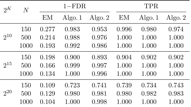
Structured latent attribute models (SLAMs) are a special family of discrete latent variable models widely used in social and biological sciences. This paper considers the problem of learning significant attribute patterns from a SLAM with potentially high-dimensional configurations of the latent attributes. We address the theoretical identifiability issue, propose a penalized likelihood method for the selection of the attribute patterns, and further establish the selection consistency in such an overfitted SLAM with a diverging number of latent patterns. The good performance of the proposed methodology is illustrated by simulation studies and two real datasets in educational assessments.
1. Introduction
Structured Latent Attribute Models (SLAMs) are widely used statistical and machine learn-ing tools in modern social and biological sciences. SLAMs offer a framework to achieve fine-grained inference on individuals’ latent attributes based on their observed multivariate responses, and also to obtain the latent subgroups of a population based on the inferred attribute patterns. In practice, each latent attribute is often assumed to be discrete and has particular scientific interpretation, such as mastery or deficiency of some targeted skill in ed-ucational assessments (Junker and Sijtsma, 2001; de la Torre, 2011), presence or absence of some underlying mental disorder in psychiatric diagnosis (Templin and Henson, 2006; de la Torre et al., 2018), and the existence or nonexistence of some disease pathogen in subjects’ biological samples (Wu et al., 2017). In these scenarios, the framework of SLAMs enables one to simultaneously achieve the machine learning task of clustering, and the scientific purpose of diagnostic inference.
Different from the exploratory nature of traditional latent variable models, SLAMs often have some additional scientific information for model fitting. In particular, the observed variables are assumed to have certain structured dependence on the unobserved latent attributes, where the dependence is introduced through a binary design matrix to respect the scientific context. The rich structure and nice interpretability of SLAMs make them popular in many scientific disciplines, such as cognitive diagnosis in educational assessment (Junker and Sijtsma, 2001; von Davier, 2008; Henson et al., 2009; Rupp et al., 2010; de la Torre, 2011), psychological and psychiatric measurement for diagnosis of mental disorders
c
(Templin and Henson, 2006; de la Torre et al., 2018), and epidemiological and medical studies for scientifically constrained clustering (Wu et al., 2017, 2018).
One challenge in modern applications of SLAMs is that the number of discrete latent attributes could be large, leading to a high-dimensional space for all the possible config-urations of the attributes, i.e., a high-dimensional space for latent attribute patterns. In many applications, the number of potential patterns is much larger than the sample size. For scientific interpretability and practical use, it is often assumed that not all the possible attribute patterns exist in the population. Examples with a large number of potential latent patterns and a moderate sample size can be found in educational assessments (Lee et al., 2011; Choi et al., 2015; Yamaguchi and Okada, 2018) and the epidemiological diagnosis of disease etiology (Wu et al., 2017). For instance, Example 1 in Section 2 presents a dataset from Trends in International Mathematics and Science Study (TIMSS), which has 13 bi-nary latent attributes (i.e., 213 = 8192 possible latent attribute patterns) while only 757 students’ responses are observed. In cognitive diagnosis, it is of interest to select the signif-icant attribute patterns among these 213= 8192 ones. In such high-dimensional scenarios, existing estimation methods often tend to over select the number of latent patterns, and may not scale to datasets with a huge number of patterns. Moreover, theoretical questions remain open on whether and when the “sparse” latent attribute patterns are identifiable and can be consistently learned from data.
Identifiability of SLAMs has long been an issue in the literature (e.g., von Davier, 2008; DeCarlo, 2011; Maris and Bechger, 2009; von Davier, 2014; Xu and Zhang, 2016). SLAMs can be viewed as a special family of restricted latent class models and their identifiability has a close connection with the study of tensor decompositions, by noting that the probability distribution of a SLAM can be viewed as a mixture of specially structured tensor products. In the literature, it is known that unrestricted latent class models are not identifiable (Gyl-lenberg et al., 1994). Nonetheless, Carreira-Perpin´an and Renals (2000) showed through extensive simulations that they are almost always identifiable, which the authors termed as practical identifiability. Allman et al. (2009) further established generic identifiability of various latent variable models, including latent class models. Generic identifiability is weaker than strict identifiability, and it implies that the model parameters are almost surely identifiable with respect to the Lebesgue measure of the parameter space. The study of All-man et al. (2009) is based on an identifiability result of the three-way tensor decomposition in Kruskal (1977). Other analysis of tensor decompositions has also been conducted to study the identifiability of various latent variable models (e.g., Drton et al., 2007; Hsu and Kakade, 2013; Anandkumar et al., 2014; Bhaskara et al., 2014; Anandkumar et al., 2015; Jaffe et al., 2018). However, the structural constraints imposed by the design matrix make these results not directly applicable to SLAMs.
In terms of estimation, learning sparse attribute patterns from a high-dimensional space is related to learning the significant mixture components in a highly overfitted mixture model. Researchers have shown that the estimation of the mixing distributions in overfitted mixture models is technically challenging and it usually leads to nonstandard convergence rate (e.g., Chen, 1995; Ho and Nguyen, 2016; Heinrich and Kahn, 2018). Estimating the number of components in the mixture model goes beyond only estimating the parameters of a mixture, by learning at least the order of the mixing distribution (Heinrich and Kahn, 2018). This problem was also studied in Rousseau and Mengersen (2011) from a Bayesian perspective; however, the Bayesian estimator in Rousseau and Mengersen (2011) may not guarantee the frequentist selection consistency, as to be shown in Section 3. In the setting of SLAMs with the structural constraints and a large number (larger than sample size) of potential latent attribute patterns, it is not clear how to consistently select the significant patterns.
Our contributions in this paper contain the following aspects. First, we characterize the identifiability requirement needed for a SLAM with an arbitrary subset of attribute patterns to be learnable, and establish mild identifiability conditions. Our new identifiability conditions significantly extends the results of previous works (Xu, 2017; Xu and Shang, 2018) to more general and practical settings. Second, we propose a statistically consistent method to perform attribute pattern selection. In particular, we establish theoretical guarantee for selection consistency in the setting of high dimensional latent patterns, where both the sample size and the number of latent patterns can go to infinity. Our analysis also shows that imposing the popular Dirichlet prior on the population proportions would fail to select the true model consistently, when the convergence rate of the SLAM is slower than the usual root-N rate. As for computation, we develop two approximation algorithms to maximize the penalized likelihood for pattern selection. In addition, we propose a fast screening strategy for SLAMs as a preprocessing step that can scale to a huge number of potential patterns, and establish its sure screening property.
The rest of the paper is organized as follows. Section 2 introduces the general setup of structured latent attribute models and motivates our study. Section 3 investigates the learnability requirement and proposes mild sufficient conditions for learnability. Section 4 proposes the estimation methodology and establishes theoretical guarantee for the proposed methods. Section 5 and Section 6 include simulations and real data analysis, respectively. The proofs of all the theoretical results and additional experimental results are included in the Appendix.
2. Model Setup and Motivation
In this section, we first describe the model setup of SLAMs and present several examples. Then we describe the motivation for our study and introduce the problem of interest.
2.1. Structured Latent Attribute Models and Examples
We first introduce the general setup of SLAMs. Consider a SLAM with J designed items which depend on theK latent attributes of interest. There are two types of subject-specific variables in the model, the observed responses to items R = (R1, . . . , RJ) and the latent
-dimensional vectorR∈ {0,1}J denotes the observed binary responses to the set ofJ items.
TheK-dimensional vectorα∈ {0,1}K denotes a profile of existence or non-existence of the
K attributes.
A key structure that specifies how the observed responses depend on the latent attributes is called theQ-matrix, which is aJ×K matrix with binary entries. We denote Q= (qj,k)
and qj,k ∈ {1,0} reflects whether or not the response to item j has statistical dependence
on attribute k. In the context of an educational assessment, qj,k = 1 implies the jth test
item requires the mastery of thekth skill attribute to answer correctly. We denote thejth row vector of Q by qj, then the K-dimensional binary vectorqj reflects the full attribute requirements of item j. For an attribute pattern α, we say α possesses all the required attributes of item j, if α qj, where α qj denotes αk ≥ qj,k for all k = 1, . . . , K.
Example 1 below gives an example of the Q-matrix.
Example 1 Trends in International Mathematics and Science Study (TIMSS) is a large scale cross-country educational assessment. TIMSS evaluates the mathematics and science abilities of fourth and eighth graders every four years since 1995. Researchers have used SLAMs to analyze the TIMSS data (e.g., Lee et al., 2011; Choi et al., 2015; Yamaguchi and Okada, 2018). For example, a 23×13 Q-matrix constructed by mathematics educators was specified for the TIMSS 2003 eighth grade mathematics assessment (Choi et al., 2015). Thirteen attributes (K = 13) are identified, which fall in five big categories of skill domains measured by the exam, Number, Algebra, Geometry, Measurement, and Data. Table 1 shows the first and last three rows of the Q-matrix, i.e., {qj :j = 1,2,3,21,22,23}.
Item α1 α2 α3 α4 α5 α6 α7 α8 α9 α10 α11 α12 α13
1 1 0 0 0 0 0 0 0 0 0 1 0 1
2 0 0 0 0 0 1 0 0 0 0 0 0 0
3 0 1 0 0 0 0 1 0 0 0 0 0 0
..
. ... ... ... ... ... ... ... ... ... ... ... ... ...
21 0 0 0 0 1 0 0 0 0 0 0 0 0
22 0 1 0 0 0 0 0 0 0 0 0 0 0
23 0 0 0 1 0 0 0 0 1 0 0 0 0
Table 1: Q-matrix, TIMSS 2003 8th Grade Data
The Q-matrix constrains the model parameters in a certain way to reflect the scientific assumptions. We next introduce the model parameters and how the Q-matrix impose constraints on them in general. Conditional on a subject’s latent attribute pattern α ∈ {0,1}K, his/her responses to the J items are assumed to be independent Bernoulli random
variables with parameters θ1,α, . . . , θJ,α. Specifically, θj,α = P(Rj = 1 | α) denotes the
positive response probability, and is also called an item parameter of item j. We collect all the item parameters in the matrixΘ= (θj,α), which has sizeJ×2K with rows indexed by
theJ items and columns by the 2K attribute patterns. For patternα∈ {0,1}K, we denote
its corresponding column vector inΘ byΘ
·
,α.One key assumption in SLAMs is that for a latent attribute pattern α = (α1, . . . , αK)
in the set Kj = {k ∈ {1, . . . , K} :qj,k = 1}; that is, those attributes related to item j as
specified in theQ-matrix. We will sometimes call the attributes inKj therequired attributes
of itemj. Under this assumption, all latent attribute patterns in the set
Cj ={α∈ {0,1}K : αqj} (1)
share the same value ofθj,α; namely,
max
α∈Cj
θj,α= min α∈Cj
θj,α for any j∈ {1, . . . , J}. (2)
We will call the setCj aconstraint set. Thus, theQ-matrix puts constraints onΘby forcing
certain entries of it to be the same. Different SLAMs model the dependence ofθj,α on the
required attributes in Kj differently to encode different scientific assumptions; please see Examples 2 and 3.
In addition to (2), another key assumption in SLAMs is the monotonicity assumption that
θj,α> θj,α0 for any α∈ Cj,α0 6∈ Cj. (3)
Constraint (3) is commonly used in our motivating applications of cognitive diagnosis in educational assessments, where (3) indicates subjects mastering all required attributes of an item are more “capable” of giving a positive response to it (i.e., with a larger Bernoulli parameterθj,α), than those who lack some required attributes. Nonetheless, our theoretical
results of model learnability in Section 3 also applies if (3) is relaxed to
θj,α6=θj,α0 for any α∈ Cj,α0 6∈ Cj.
This allows more flexibility in the model assumptions of SLAMs used in other applications. Next we introduce some popular SLAMs in educational and psychological applications. These models are also called Cognitive Diagnosis Models in the psychometrics literature. The first type of SLAMs have exactly two item parameters associated with each item.
Example 2 (two-parameter SLAM) The two-parameter SLAM specifies exactly two item parameters for each itemj, which we denote byθj+ andθj−, withθ+j > θj−. The popular De-terministic Input Noisy output “And” gate (DINA) model introduced in Junker and Sijtsma (2001) is a two-parameter SLAM. It specifies the general form of θj,α can be rewritten as
θtwo-param.j,α =
(
θ+j , if α∈ Cj,
θ−j , if α6∈ Cj.
In the application of the two-parameter SLAM in educational assessments, the item pa-rameters θj+ and θ−j have the following interpretations. The 1−θ+j is called the slipping parameter, denoting the probability of a “capable” subject slips the correct answer, despite mastering all the required attributes of the test itemj; andθ−j is called the guessing param-eter, denoting the probability of a “non-capable” subject coincidentally giving the correct answer by guessing, despite lacking some required attributes of item j. In this case, the unique item parameters in matrix Θ reduce to (θ+,θ−), where θ+ = (θ1+, . . . , θ+J)> and
Another family of SLAMs are the multi-parameter models, which allow each item to have multiple levels of item parameters.
Example 3 (multi-parameter SLAMs) Multi-parameter SLAMs can be categorized into two general types, the main-effect models and the all-effect models. The main-effect models assume the main effects of the required attributes in Kj play a role in distinguishing the item parameters, which can be written as
θj,αmain-eff=f
βj,0+ X
k∈Kj
βj,kαk
, (4)
wheref(·)is a link function. Different link functionsf(·)lead to different models, including the popular reduced Reparameterized Unified Model (reduced-RUM; DiBello et al., 1995) with f(·) being the exponential function, the Linear Logistic Model (LLM; Maris, 1999) with f(·) being the sigmoid function, and the Additive Cognitive Diagnosis Model (ACDM; de la Torre, 2011) with f(·) the identity function.
Another type of multi-parameter SLAMs are the all-effect models. The item parameter of an all-effect model can be written as
θall-effj,α =fX
S⊆Kj
βj,S
Y
k∈Sαk
. (5)
Whenf(·)is the identity function,(5)gives the Generalized DINA (GDINA) model proposed by de la Torre (2011); and when f(·) is the sigmoid function, (5) gives the Log-linear Cognitive Diagnosis Models (LCDMs) proposed by Henson et al. (2009); see also the General Diagnostic Models (GDMs) proposed in von Davier (2008).
Under the multi-parameter SLAMs, the constraint set of each itemj also takes the form of (1). Those attribute patterns in Cj still share the same value of item parameters by
the definition; and what is different from the two-parameter counterpart is that those α not in Cj can have different levels of item parameters. We next give another example of multi-parameter SLAMs.
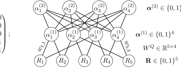
Example 4 (Deep Boltzmann Machines) The Restricted Boltzmann Machine (RBM) (Smolensky, 1986; Goodfellow et al., 2016) is a popular neural network model. RBM is an undirected probabilistic graphical model, with one layer of latent (hidden) binary variables, one layer of observed (visible) binary variables, and a bipartite graph structure between the two layers. We denote variables in the observed layer byRand variables in the latent layer by α, with lengths J and K, respectively. Under an RBM, the probability mass function of R and α is P(R,α) ∝ exp(−R>WQα−f>R−b>α), where f, b, and WQ = (wj,k)
are the parameters. The binary Q-matrix then specifies the sparsity structure in WQ, by constraining wj,k 6= 0 only if qj,k 6= 0. The Deep Boltzmann Machine (DBM) is a
generalization of RBM by allowing multiple latent layers. Consider a DBM with two latent layers α(1) and α(2) of length K1 and K2, respectively. The probability mass function of
(R,α(1),α(2)) in this DBM can be written as P(R,α(1),α(2))∝exp
where f ∈ RJ, b
i ∈ RKi for i = 1,2, and WQ = (wj,k) ∈ RJ×K1, U ∈ RK1×K2 are model parameters; Figure 1 gives an example of a DBM with a 5×4 Q-matrix. For f = (f1, . . . , fJ)>andα(1) = (α
(1) 1 , . . . , α
(1)
K1), the conditional distribution of an observed variable Rj given the latent variables is
P(Rj = 1|α(1),α(2),· · ·) =P(Rj = 1|α(1)) =
expPK1
k=1wj,kα (1)
k +fj
1 + exp
PK1
k=1wj,kα (1)
k +fj
, (7)
where “· · ·” represents deeper latent layers that potentially exist in a DBM. Moreover, from
(6) we have P(R | α(1)) = QjJ=1P(Rj | α(1)), so a DBM satisfies the local independence
assumption that the Rj’s are conditionally independent given the α(1). Therefore, a DBM
can be viewed as a multi-parameter main-effect SLAM in (4)with a sigmoid link function. Viewing a DBM in this way, (7) gives the item parameter θj,α(1), and the constraint set of each item j also takes the formCj ={α(1)∈ {0,1}K1 : α(1) qj}.
Q=
1 0 1 0
1 1 0 0
0 1 1 0
0 0 1 1
0 1 0 1
;
R1 R2 R3 R4 R5 R∈ {0,1}5 α(1)1 α2(1) α(1)3 α(1)4 α(1) ∈ {0,1}4
WQ∈R5×4 w1
,1 w5,
4
α(2)1 α(2)2 α(2)3 α(2)4 α(2)∈ {0,1}4
Figure 1: Deep Boltzmann Machine
2.2. Motivation and Problem
One challenge in modern applications of SLAMs is that the number of potential latent attribute patterns 2K increases exponentially with K and could be much larger than the sample sizeN. It is often assumed that a relatively small portion of attribute patterns exist in the population. For instance, Example 1 has 2K = 213 = 8192 different configurations of attribute patterns; for the limited sample size 757 there, it is desirable to learn the potentially small set of significant attribute patterns from data.
Another motivation for assuming a small number of attribute patterns exist in the population results from the possible hierarchical structure among the targeted attributes. For instance, in an educational assessment of a set of underlying latent skill attributes, some attributes often serve as prerequisites for some others (Leighton et al., 2004; Templin and Bradshaw, 2014). Specifically, the prerequisite relationship depicts the different level of difficulty of the skill attributes, and also reveals the order in which these skills are learned in the population of students. For instance, if attribute α1 is a prerequisite for attribute
α2, then the attribute pattern (α1 = 0, α2 = 1) does not exist in the population, naturally
desirable to learn the hierarchy of attributes directly from data. In such cases with attribute hierarchy, the number of patterns respecting the hierarchy could be far fewer than 2K.
The problem of interest is that, given a moderate sample size, how to consistently esti-mate the small set of latent attribute patterns among all the possible 2Kones. As discussed in the introduction, in the high-dimensional case when the total number of attribute pat-terns is large or even larger than the sample size, the questions of when the true model with the significant latent patterns are learnable from data, and how to perform consistent pattern selection, remain open in the literature.
This problem is equivalent to selecting the nonzero elements of the population proportion parameters p= (pα : α ∈ {0,1}K), where pα denotes the proportion of the subjects with
latent pattern α in the population. The p satisfies pα ∈ [0,1] for all α ∈ {0,1}K and
P
α∈{0,1}Kpα = 1. In this work, we will treat the latent attribute patterns α as random
variables (random effects). For any subject, his/her attribute pattern is a random vector
A∈ {0,1}K that (marginally) follows a categorical distribution with population proportion
parameters p = (pα : α ∈ {0,1}K). One main reason for this random effect assumption
is that, when the number of observed variables per subject (i.e.,J) does not increase with the sample size N asymptotically, the counterpart fixed effect model can not consistently estimate the model parameters. As a consequence, the fixed effect approach can not give consistent selection of significant attribute patterns. This scenario with relatively small J
but larger N and 2K is commonly seen in the motivating applications in educational and psychological assessments.
We would like to point out that we give the joint distribution of the attributes full flexibility by modeling it as a categorical distribution with 2K−1 free proportion parameters
pα’s. Modeling in this way allows those “sparse” significant attribute patterns to have
arbitrary structures among the 2K possibilities. On the contrary, any simpler parametric model of the distribution ofαwith fewer parameters would fail to capture all the possibilities of the attributes’ dependency.
Under the introduced notations, the probability mass function of a subject’s response vectorR= (R1, . . . , RJ)>can be written asP(R=r|Θ,p) =Pα∈{0,1}KpαQJj=1θ
rj
j,α(1−
θj,α)1−rj,forr∈ {0,1}J.Alternatively, the responses can be viewed as aJ-th order tensor
and the probability mass function of Rcan be written as a probability tensor
P(R|Θ,p) = 2K
X
l=1 pαl
θ1,αl 1−θ1,αl
◦
θ2,αl 1−θ2,αl
◦ · · · ◦
θJ,αl 1−θJ,αl
, (8)
where “◦” denotes the tensor outer product andθj,α’s are constrained by (2) and (3).
In the following sections, we first investigate the learnability requirement of learning a SLAM with an arbitrary set of true latent patterns, and provide identifiability conditions in Section 3. Then in Section 4, we propose a penalized likelihood method to select the latent attribute patterns, and establish theoretical guarantee for the proposed method.
3. Learnability Requirement and Conditions
by theQ-matrix. The rows of Γallare indexed by theJ items, and columns by the 2K latent attribute patterns in {0,1}K. The (j,α)th entry of Γall
j,α is defined as
Γallj,α=I(αqj) =I(α∈ Cj), j∈ {1, . . . , J}, α∈ {0,1}K, (9)
which is a binary indicator of whether attribute patternαpossess all the required attributes of item j. We will also call Γall theconstraint matrix, since its entries indicate what latent patterns are constrained to have the highest level of Bernoulli parameters for each item. For example, consider the 2×2 Q-matrix in the following (10). Then its corresponding Γ-matrix Γall with a saturated set of attribute patterns takes the following form.
Q=
0 1
1 1
=⇒ Γall =
α1 α2 α3 α4
(0,0) (0,1) (1,0) (1,1)
0 1 0 1
0 0 0 1
. (10)
More generally, we generalize the definition of the constraint matrix Γallin (9) to an arbitrary subset of latent patterns A ⊆ {0,1}K, and an arbitrary set of items S ⊆[J]. For S ⊆[J]
and A ⊆ {0,1}K, we simply denote by Γ(S,A) the |S| × |A| submatrix of Γall with row
indices from S and column indices from A. When S ={1, . . . , J}, we will sometimes just denote Γ(S,A) by ΓA for simplicity. Then ΓA itself can be viewed as the constraint matrix
for a SLAM with attribute pattern space A, and ΓA directly characterizes how the items constrain the positive response probabilities of latent attribute patterns inA.
Given the Q-matrix, we denote by A0 ⊆ {0,1}K the set of true attribute patterns
existing in the population, i.e., A0 ={α ∈ {0,1}K :pα > 0}. In knowledge space theory
(D¨untsch and Gediga, 1995), the setA0 of patterns corresponds to theknowledge structure
of the population. We further denote by ΘA0 the item parameter matrix respecting the
constraints imposed by ΓA0; specifically, ΘA0 = (θ
j,α) has the same size as ΓA0, with
rows and columns indexed by the J items and the attribute patterns in A0, respectively. For any positive integer k ≤ 2K, we let Tk−1 be the k-dimensional simplex, i.e., Tk−1 = {(x1, x2, . . . , xk) : xi ≥ 0, Pki=1xk = 1}. We denote the true proportion parameters by
pA0 = (p
α,α∈ A0)∈ T|A0|−1, thenpA0 0by the definition of A0.
The following toy example illustrates why we need to establish identifiability guarantee for pattern selection.
Example 5 Consider the2×2 Q-matrix together with its corresponding2×4 Γ-matrix in Equation (10). Consider two attribute pattern sets, the true set A0 = {α1 = (0,0),α2 =
(0,1)} and an alternative set A1 = {α2 = (0,1),α3 = (1,0)}. Under the two-parameter SLAM, for any valid item parameters Θ restricted by Γ and any proportion parameters
p= (pα1, pα2, pα3, pα4)such that pα1 =pα3, we have P(R=r|Θ
A0,(p
α1, pα2)) =P(R=
r|ΘA1,(p
α3, pα2)).This is becauseΓ
A0 = ΓA1 from (10)and henceΘA0 =ΘA1; and also
From the above example, to make sure the set of true attribute patternsA0 is learnable from the observed multivariate responses, we need the ΓA0-matrix to have certain structures.
We state the formal definition of (strict) learnability of A0.
Definition 1 (strict learnability of A0) Given Q, the set A0 is said to be (strictly) learnable, if for any constraint matrix ΓA of size J × |A| with |A| ≤ |A0|, any valid item parameters ΘA respecting constraints given by ΓA, and any proportion parameters
pA∈ T|A|−1, pA0, the following equality
P(R|ΘA0,pA0) =P(R|ΘA,pA) (11) implies A=A0. Moreover, if (11)implies (ΘA,pA) = (ΘA0,pA0), then we say the model parameters (ΘA0,pA0) are (strictly) identifiable.
Next we further introduce some notations and definitions about the constraint matrix Γ and then present the needed identifiability result. Consider an arbitrary subset of items
S ⊆ {1, . . . , J}. For α,α0 ∈ A, we denote α S α0 under ΓA, if for each j ∈ S there is ΓAj,α ≥ ΓAj,α0. If viewing Γj,α = 1 as α being “capable” of item j, then α S α0 would
meanα is at least as capable asα0 of items in set S. Then under Γ, any subset of itemsS
defines a partial order “S” on the set of latent attribute patternsA. For two item setsS1
and S2, we say “S1 ” = “S2 ” under Γ
A, if for any α0,α∈ A, there is α S1 α
0 under
ΓA if and only if α S2 α
0 under ΓA. The next theorem gives conditions that ensure the
constraint matrix Γ as well as the Γ-constrained model parameters are jointly identifiable.
Theorem 2 (conditions for strict learnability) Consider a SLAM with an arbitrary set of true attribute patterns A0 ⊆ {0,1}K, and a corresponding constraint matrix ΓA0. If this true ΓA0 satisfies the following conditions, then A
0 is identifiable.
A. There exist two disjoint item sets S1 and S2, such that Γ(Si,A0) has distinct column vectors for i= 1,2 and “S1=S2” underΓ
A0.
B. For any α, α0 ∈ A0 where α0 Si α under ΓA0 for i = 1 or 2, there exists some j∈(S1∪S2)c such that ΓA0
j,α6= Γ A0
j,α0.
C. Any column vector of ΓA0 is different from any column vector of ΓAc0, where Ac 0 = {0,1}K\ A
0.
Recall that each column in the Γ-matrix corresponds to a latent attribute pattern, then Conditions A and B help ensure the Γ-matrix of the true patterns ΓA0 contains enough
information to distinguish between these true patterns. Specifically, Condition A requires ΓA0 to contain two vertically stacked submatrices corresponding to item sets S1 and S2,
each having distinct columns, i.e., each being able to distinguish between the true patterns; and Condition B requires the remaining submatrix of ΓA0 to distinguish those pairs of
true patterns that have some order (α0 Si α) based on the first two item sets S1 orS2. Condition C is necessary for identifiability of A0 by ensuring that any true pattern would
have a different column vector in Γall from that of any false pattern. ConditionCis satisfied for any A0 ⊆ {0,1}K if the Q-matrix contains an identity submatrix IK, because such a
We would like to point out that our identifiability conditions in Theorem 2 do not depend on the unknown parameters (e.g., Θand p), but only rely on the structure of the constraint matrix Γ. The Γ-matrix with respect to the true set of patterns A0 is the key quantity that defines the latent structure of a SLAM. Generally, it is hard to establish identifiability conditions that only depend on the cardinality of A0 but not on ΓA0. For
instance, in Example 5, the two sets A0 and A1 have the same cardinality but can not be distinguished under the conditions there; indeed further conditions onQ(and the resulting Γ) are needed to guarantee identifiability.
The developed identifiability conditions generally apply to any SLAM satisfying the constraints (2) and (3) introduced in Section 2.1. If one makes further assumptions on Θ, such as assuming each item j ∈ [J] has exactly two item parameters to make it a two-parameter model, then the conditions in Theorem 2 may be further relaxed. For example, in the saturated case with A0 ={0,1}K, the sufficient identifiability conditions developed
in Xu (2017) for a general SLAM require Q to contain two copies of IK as submatrices,
while the necessary and sufficient conditions established in Gu and Xu (2019a) for the two-parameter SLAM require Qto have just one submatrixIK. We expect that in the current
case with an arbitraryA0 ⊆ {0,1}K, the conditions in Theorem 2 can also be relaxed under
the two-parameter model in a technically nontrivial way. For the reason of generality, we focus on SLAMs under the general constraints (2) and (3) in this work.
When the conditions in Theorem 2 are satisfied, A0 is identifiable; and from Theorem
4.1 in Gu and Xu (2019b), the model parameters (ΘA0,pA0) associated with A
0 are also
identifiable.
Corollary 3 Under the conditions in Theorem 2, the model parameters (ΘA0,pA0) asso-ciated with A0 are identifiable.
Note that the result of Theorem 2 differs from the existing works Xu (2017), Xu and Shang (2018) and Gu and Xu (2019b) in that those works assumeA0 is knowna priori and study the identifiability of (ΘA0,pA0), while in the current work A
0 is unknown and we focus on
the identifiability of A0 itself. This is crucially needed in order to guarantee that we can learn the set of true attribute patterns.
Remark 4 The identifiability results in Theorem 2 and Corollary 3 are related to the uniqueness of tensor decomposition. As shown in (8), the probability mass function of the multivariate responses of each subject can be viewed as a higher order tensor with constraints on entries of the tensor, and unique decomposition of the tensor correspond to identifica-tion of the constraint matrix as well as the model parameters. The identifiability condiidentifica-tions in Theorem 2 are weaker than the general conditions for uniqueness of three-way tensor decomposition in Kruskal (1977), which is a celebrated result in the literature. Kruskal’s conditions require the tensor can be decomposed as a Khatri-Rao product of three matrices, two having full-rank and the other having Kruskal rank at least two (Kruskal rank of a matrix is the largest number T such that every set of T columns of it are linearly indepen-dent). Consider an example with J = 5, K = 2, A0 ={α2 = (0,1), α3 = (1,0)}, and the corresponding ΓA0 in the form of (12). Then we can set S
1 ={1,2}, S2 ={3,4}and Con-dition A in Theorem 2 is satisfied. Further, Condition B is also satisfied since α2 Si α3
and α3 Si α2 under Γ
A0. Therefore, Theorem 1 guarantees the set A
and further guarantees the parameters (ΘA0,pA0) are identifiable. On the contrary, results based on Kruskal’s conditions for unique three-way tensor decomposition can not guarantee identifiability, because other than two full rank structures given by the items in S1 and S2, the remaining item 5 in(S1∪S2)ccorresponds to a structure with Kruskal rank only one.
Q=
1 0
0 1
1 0
0 1
1 1
=⇒ ΓA0 =
α2 α3
(0,1) (1,0)
1 0
0 1
1 0
0 1
0 0
. (12)
We next discuss two extensions of the developed identifiability theory. First, Theorem 2 guarantees the strict learnability of A0. Under a multi-parameter SLAM, these conditions can be relaxed if the aim is to obtain the so-called generic joint identifiability of A0, which
means that A0 is learnable with the true model parameters ranging almost everywhere in
the constrained parameter space except a set with Lebesgue measure zero. Specifically, we have the following definition.
Definition 5 (generic learnability of the true model) Denote the parameter space of
(ΘA0,pA0) constrained by ΓA0 by Ω. We say A
0 is generically identifiable, if there exists a subset V of Ω that has Lebesgue measure zero, such that for any (ΘA0,pA0) ∈ Ω\ V, Equation (11) implies A = A0. Moreover, if for any (ΘA0,pA0) ∈ Ω\ V, Equation (11) implies (ΘA,pA) = (ΘA0,pA0), we say the model parameters (ΘA0,pA0) are generically identifiable.
The generic learnability result is presented in the next theorem.
Theorem 6 (conditions for generic learnability) Consider a multi-parameter SLAM with the set of true attribute patterns A0 and the J × |A0| constraint matrix ΓA0. If ΓA0 satisfies Condition C and also the following conditions, thenA0 is generically identifiable. A?. There exist two disjoint item sets S1 and S2, such that altering some entries from 0
to 1 in Γ(S1∪S2,A0) can yield a e
Γ(S1∪S2,A0) satisfying Condition A. That is, e
Γ(Si,A0)
has distinct columns for i= 1,2 and “S1 ” = “S2 ” under eΓ
(S1∪S2,A0). B?. For any α, α0 ∈ A0 where α0 Si α under eΓ
(S1∪S2,A0) for i = 1 or 2, there exists some j∈(S1∪S2)c such thatΓA0
j,α6= Γ A0
j,α0.
We also have the following corollary, where the identifiability requirements are directly characterized by the structure of the Q-matrix, instead of Γ.
(A??) The Q contains two K×K sub-matrices Q1, Q2, such that for i= 1,2,
Q=
Q1 Q2 Q0
J×K
; Qi =
1 ∗ . . . ∗ ∗ 1 . . . ∗
..
. ... . .. ...
∗ ∗ . . . 1
K×K
, i= 1,2, (13)
where each ‘∗’ can be either zero or one.
(B??) With Q in the form of (13), there is PJ
j=2K+1qj,k ≥1 for each k∈ {1, . . . , K}.
Remark 8 When the conditions in Theorem 7 are satisfied, A0 is generically identifiable and from Theorem 4.3 in Gu and Xu (2019b), the model parameters (ΘA0,pA0) are also generically identifiable. Corollary 7 differs from Theorem 4.3 in Gu and Xu (2019b) in that, here we allow the true set of attribute patterns A0 to be unknown and arbitrary, and study its identifiability, while Gu and Xu (2019b) assumes A0 is pre-specified and studies the identifiability of the model parameters (ΘA0,pA0).
Remark 9 Under the conditions for generic identifiability in Theorem 6 or Corollary 7, we can obtain the explicit forms of the measure zero setV (V ⊆Ω) where the non-identifiability may occur. Under either Theorem 6 or Corollary 7, the set V is characterized by the zero set of certain polynomials about the parameters (Θ,p) (see the proofs for details). The zero set of these polynomials indeed defines a lower-dimensional manifold in the parameter space. Therefore, Theorem 6 and Corollary 7 supplement Theorem 2 by relaxing the original conditions and establishing identifiability when(Θ,p) satisfy certain shape constraints, i.e.,
(Θ,p) do not fall on that manifold V in the parameter space.
The above generic identifiability results of A0 ensure that nonidentifiability happens
only in a measure zero set in the parameter space. Next, we develop a second extension of Theorem 2 for scenarios where nonidentifiability cases occupy a positive measure set in the parameter space. This situation happens when certain latent attribute patterns always have the same item parameters across all the items, i.e., Θ
·
,α =Θ·
,α0 for some α 6= α0.We define α and α0 to be in the same equivalence class if Θ
·
,α = Θ·
,α0. For instance,still consider the following 2×2 Q-matrix under the two-parameter SLAM introduced in Example 2,
Q=
0 1 1 1
, (14)
then attribute patternsα1 = (0,0) andα3 = (1,0) are equivalent under the two-parameter
SLAM, as can be seen from the Γall in (10). Therefore the two latent patternsα1 and α3
are not identifiable, no matter which values the true model parameters take.
equivalent, there are three equivalence classes: {α1 = (0,0),α3 = (1,0)}, {α2 = (0,1)},
and {α4 = (1,1)}. We denote these three equivalence classes by [α1] (or [α3], since [α1] =
[α3]), [α2] and [α4], since α1, α2 and α4 form a complete set of representatives of the
equivalence classes. For anyQ, we denote the induced set of equivalence classes byAequiv= {[α1], . . . ,[αC]}, whereα1, . . . ,αC form a complete set of representatives of the equivalence
classes. In this case, the pattern selection problem of interest is to learn which equivalence classes inAequiv are significant.
For the two-parameter SLAM introduced in Example 2, two attribute patterns α1,α2
are in the same equivalence class if and only if ΓA·,α1 = Γ
A
·,α2. This is because under the
two-parameter SLAM, the Γ-matrix determined by the Q-matrix with Γj,α =I(α qj) fully
captures the model structure in the sense thatθj,α=θj+Γj,α+θj−(1−Γj,α). Therefore under
a two-parameter SLAM, we can obtain a complete set of representatives of the equivalence classes directly from the q-vectors, which are
AQ={∨j∈Sqj : S ⊆ {1, . . . , J}}, (15)
where ∨j∈Sqj = (maxj∈S qj,1, . . . ,maxj∈S qj,K). For S =∅, we define the vector ∨j∈Sqj
to be 0K, the all-zero attribute pattern. The reasons for AQ being a complete set of
representatives are that, first, ΓAQ has distinct columns and contains all the unique column vectors in Γall; and second, for any other pattern not in AQ, there is some pattern in AQ
such that the two patterns have identical column vectors in Γall. It is not hard to see that
AQ={0,1}K if and only if the Q-matrix contains a submatrix I K.
For multi-parameter SLAMs introduced in Example 3, two attribute patterns α1,α2
are in the same equivalence class if Γ·,α1 = Γ·,α2 = 1. This can be seen by considering
Γ·,α1 = Γ·,α1 6= 1, i.e., Γj,α1 = Γj,α2 = 0 for some item j. Then different from the
two-parameter SLAMs, for such item j, the θj,α1 and θj,α2 are not always the same by
the modeling assumptions of multi-parameter SLAMs. Indeed, under a multi-parameter SLAM, for item j, patterns in the setA0\ Cj can have multiple levels of item parameters.
We have the following corollary of Theorem 2 on identifiability, when certain attribute patterns are not distinguishable. Denote the set of significant equivalence classes byAequiv0 =
{[α`1], . . . ,[α`m]}, which is a subset of the saturated set A
equiv={[α
1], . . . ,[αC]}. Denote
the set of representative patterns of the significant equivalence classes by{α`1, . . . ,α`m}=
Arep.
Corollary 10 If the matrix ΓArep satisfies ConditionsA,B andC, Aequiv0 is identifiable. Remark 11 Under the two-parameter SLAM withAequiv ={[α
1], . . . ,[αC]}, the Γ-matrix
Γ{α1,...,αC} by definition would have distinct column vectors. Therefore any column vector
of ΓArep in Corollary 10 must be different form any column vector of Γ{α1,...,αC}\Arep. In
this case, Condition C is automatically satisfied. And in order to identify Aequiv0 , one only needs to check if ΓArep satisfies ConditionsA and B.
4. Penalized Likelihood approach to pattern selection
4.1. Shrinkage Estimation
The developed identifiability conditions guarantee that the true set of patterns can be distinguished from any alternative set that has not more than |A0| patterns, since they would lead to different probability mass functions of the responses. AsA0 ={α∈ {0,1}K: pα>0}, we know that learning the significant attribute patterns is equivalent to selecting
the nonzero elements of the population proportion vector p. In practice, if we directly overfit the data with all the 2K possible attribute patterns, the corresponding maximum
likelihood estimator (MLE) can not correctly recover the sparsity structure of the vector p. In this case, we propose to impose some regularization on the proportion parameters p, and perform pattern selection through maximizing a penalized likelihood function.
In general, we denote by Ainput the set of candidate attribute patterns given to the shrinkage estimation method as input. If the saturated space of all the possible attribute patterns are considered, then Ainput={0,1}K and it contains all the 2K possible
configu-rations of attributes. When 2K N,we propose to use a preprocessing step that returns a proper subsetAinput of the saturated set{0,1}K as candidate attribute patterns, and then
perform the shrinkage estimation (please see Section 4.2 for the preprocessing procedure). We first introduce the general data likelihood of a structured latent attribute model. Given a sample of size N, we denote the ith subject’s response by Ri = (Ri,1, . . . , Ri,J)>,
i = 1, . . . , N. We further use R to denote the N ×J data matrix (R>1, . . . ,R>N)>. The marginal likelihood can be written as
L(Θ,p| R) =
N
Y
i=1
h X
α∈Ainput pα
J
Y
j=1 θRi,j
j,α(1−θj,α)1−Ri,j
i
, (16)
where the constraints onΘimposed byQare made implicit. We denote the corresponding log likelihood by `(Θ,p) = logL(Θ,p| R).
As the proportion parameters pbelongs to a simplex, in order to encourage sparsity of p, we propose to use a log-type penalty with a tuning parameterλ <0. Specifically, we use the following penalized likelihood as the objective function,
`λ(Θ,p) = `(Θ,p) +λ X
α∈Ainput
logρN(pα), λ∈(−∞,0), (17)
where logρN(pα) = log(pα)·I(pα> ρN) + log(ρN)·I(pα≤ρN) andρN is a small threshold
parameter that is introduced to circumvent the singularity issue of the log function at zero. Specifically, we take
ρN N−d (18)
for some constant d ≥ 1, where for two sequences {aN} and {bN}, we denote aN . bN
if aN = O(bN) and aN bN if aN . bN and bN . aN. Any attribute pattern α whose
estimated pα< ρN will be considered as 0, and hence not selected. The tuning parameter
λ∈(−∞,0) controls the sparsity level of the estimated proportion vector p, and a smaller
λleads to a sparser solution (with more estimated proportionpα falling belowρN). Given
Remark 12 In the literature, Chen et al. (2001) and Chen et al. (2004) used a similar form of penalty as the summation term in our (17), but instead imposed λ > 0 to avoid sparse solutions of the proportion parameters. These works used that penalty in order to avoid singularity when performing restricted likelihood ratio test. While our goal here is to encourage sparsity of pso that significant attribute patterns can be selected.
The formulation of (17) can also be interpreted in a Bayesian way, where the penalty term regarding the proportionspis the logarithm of the Dirichlet prior density with hyperpa-rameterβ =λ+ 1over the proportions. But note that whenβ <0, the penalty term is not a proper prior density. Our later Proposition 15 reveals that, under nonstandard convergence rate of the mixture model, the traditional Bayesian way of imposing a proper Dirichlet prior over proportions is not sufficient for selecting significant attribute patterns consistently. In-stead, this classical procedure will yield too many false patterns being selected. Therefore, our novelty of allowing λ in (17) to be negative with arbitrarily large magnitude is crucial to selection consistency.
Other than the nice connection to the Dirichlet prior density in the Bayesian litera-ture, the log-type penalty in (17)also facilitates the computation based on modified EM and variational EM algorithms, as shown in our Algorithms 1 and 2. For such reasons, this work uses the log-type penalty. There are also alternative ways of imposing penalty on the proportion parameters p that would lead to selection consistency, such as the truncated L1 penalty used in Shen et al. (2012) for high-dimensional feature selection.
We denote the MLE obtained from directly maximizing L(Θ,p | R) in (16) by Θb and b
p, and denote the “oracle” MLE of the parameters obtained by maximizing the likelihood constrained to the true set of attribute patterns by (Θb
A0
,bpA0). We denote the rate of
convergence of`(Θ,b p) tob `(Θb
A0
,bpA0) by δ∈(0,1], that is,
`(Θ,b bp)−`(Θb
A0 ,bp
A0)
/N =OP(N−δ). (19)
When δ = 1, (19) implies `(Θ,b bp) converges with the usual root-N rate, and δ <1 would
imply a slower convergence rate. In the literature, Ho and Nguyen (2016) and Heinrich and Kahn (2018) have studied the technically involved problem of convergence rate of the mixing distribution of certain mixture models, and showed these models may not have the standard root-N rate. As implied by these works, for complicated models like SLAMs, the convergence rate of the mixing distribution is likely to be slower than root-N, so as the convergence rate of `(Θ,b bp).
For a set A, denote its cardinality by|A|. We have the following theorem.
Theorem 13 (selection consistency) Suppose the true constraint matrixΓA0 associated with A0 satisfies conditionsA,B and C in Theorem 2. The true parameters satisfy
min
α∈A0
pα> c0; θj,α?− max
α: Γj,α=0
θj,α≥c1, ∀ j= 1, . . . , J and α?∈ Cj, (20)
wherec0, c1 >0are some constants. Assumelog|Ainput|=o(N)and|Ainput|·ρN =O(N−δ).
Then there exist a sequence of tuning parameters {λN} satisfying N1−δ/|logρN|.−λN .
Remark 14 Together with our identifiability result in Theorem 2, the assumption (20)
helps distinguish the true patterns from any alternative set of patterns with no larger cardi-nality, and further helps establish selection consistency. It is possible to further extend the current result and relax the constant lower bound assumption, though identifiability condi-tions would need to be adapted carefully to the case with a growing number of significant patterns and a shrinking magnitude of the proportions; we leave this for future work.
The proof of Theorem 13 also reveals that if the convergence rate of UN are slower
than √N with δ < 1 in (19), then the tuning parameter λ in (17) has to satisfy λ < −1 in order to have pattern selection consistency; otherwise the issue of over selecting exists. Under the Bayesian interpretation as discussed in Remark 12, this result implies that imposing the popular Dirichlet prior with a proper hyperparameterβ =λ+ 1∈(0,1) is not sufficient for consistent selection of the significant mixture components (i.e., latent attribute patterns). Therefore, the approach proposed by Rousseau and Mengersen (2011) would not yield frequentist selection consistency in this considered scenario. We state this in the following proposition.
Proposition 15 (selection inconsistency of Dirichlet prior) Suppose δ < 1 in (19), i.e., the rate of convergence of `(Θ,b p)b is slower than the usual
√
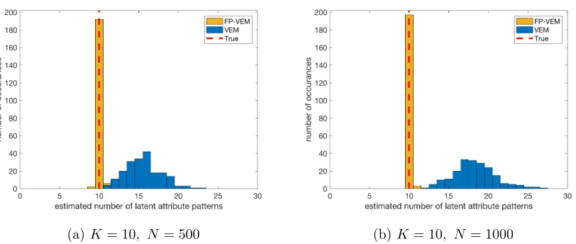
N-rate. Then there does not exist a sequence of{λN, N = 1,2, ...} ⊆[−1,0)such thatP(AbλN =A0)→1asN → ∞. Example 6 To visualize how the numbers of selected patterns differ for our proposed method based on maximizing (17) with β=λ+ 1∈(−∞,1), and the variational EM algorithm re-sulting from imposing a proper Dirichlet prior over the proportions, we conduct a simulation study. In a simulation setting of K = 10 and J = 30, for each sample size N = 500 and
1000, we carry out 200 independent runs and in each run record the number of selected attribute patterns given by the proposed method, and that by the variational EM algorithm. We plot the histogram corresponding to the proposed method (FP-VEM, see Section 4 for details), together with that corresponding to Variational EM (VEM) with a small Dirichlet parameter β = 0.01. For both algorithms, we use the same threshold ρN = 1/(2N) for
selecting attribute patterns in the end of the algorithm, by only keeping patterns whose pos-terior means exceeds ρN. Here we did not plot the results corresponding to VEM with β
smaller than 0.01, because we found the VEM algorithm with smaller β values can have convergence issues and in many cases it fails to converge but just jumps between several solutions. One can see from Figure 2 that the proposed method selects 10 patterns for most of datasets, which are indeed the 10 true patterns; while VEM over selects the patterns.
We next propose two algorithms to perform pattern selection, one being a modification of an EM algorithm, and the other being a variational EM algorithm resulting from an alternative formulation of the problem.
4.1.1. Modified EM algorithm.
(a)K= 10, N= 500 (b)K= 10, N= 1000
Figure 2: Histograms of estimated number of latent attribute patterns. VEM represents Variational EM withβ =λ+ 1 = 0.01, and FP-VEM represents the proposed Algorithm 2 in Section 4. The true number of latent attribute patterns is |A0|= 10.
(Ai,1, . . . , Ai,K), then Ai ∈ {0,1}K. The complete log likelihood corresponding to (17) is
`λcomp(Θ,p| R,A) = X
αl∈Ainput X
i
I(Ai =αl) +λ
logρN(pαl) (21)
+ X
αl∈Ainput X
i
I(Ai =αl)
X
j
h
Ri,jlog(θj,αl) + (1−Ri,j) log(1−θj,αl)
i ,
whereI(·) denotes the binary indicator function. Following the standard formulation of the EM algorithm (Dempster et al., 1977), in the E step of the (t+ 1)-th iteration, conditional expectations of `λcomp(Θ,p| R,A) is evaluated with respect to the posterior distribution of latent variables Ai’s given the current iterates of parameters Θ(t) and p(t). Specifically, in
the E step we replace the indicator I(Ai = αl) in (21) by the probability ϕi,l =P(Ai =
αl |Θ(t),p(t)); and this is equivalent to updating
Q(Θ,p|Θ(t),p(t)) :=E h
`λcomp(Θ,p| R,A)
Θ
(t),p(t)i.
In the M step, we update (Θ(t+1),p(t+1)) = arg maxQ(Θ,p|Θ(t),p(t)). Note that directly
using a negative λ in the EM algorithm may yield an invalid E step, due to potentially negative updates for some proportion parameters (e.g., pα’s). When this happens, we
do a thresholding in the E step as an approximation by replacing the probably negative class potential (∆l in Algorithm 1) with a pre-specified small constant c > 0. In practice,
Algorithm 1’s performance appears not sensitive to small values of c, and we takec= 0.01 in our numerical experiments; see Appendix B for a sensitivity study of the parameter c.
Algorithm 1:PEM: Penalized EM for log-penalty with λ∈(−∞,0)
Data: Q, responsesR, and candidate attribute patterns Ainput.
Initialize ∆= (∆(0)1 , . . . ,∆(0)|A
input|). while not converged do
In the (t+ 1)th iteration,
for(i, l)∈[N]×[|Ainput|]do
ϕ(i,αt+1)
l =
∆(lt)·expnP
j
h
Ri,jlog(θ(j,αt)l) + (1−Ri,j) log(1−θ
(t)
j,αl)
io
P
m∆
(t)
m ·exp
n P
j
h
Ri,jlog(θj,α(t)m) + (1−Ri,j) log(1−θ
(t)
j,αm)
io;
forl∈[|Ainput|]do
∆(lt+1)= max{c, λ+PN
i=1ϕ (t+1)
i,αl }; (c >0 is pre-specified); p(t+1)←∆(t+1)/(P
l∆
(t+1)
l );
forj∈[J]do Θ(t+1)=
arg maxΘ
n P
αl
P
iϕ
(t+1)
i,αl
P
j
h
Ri,jlog(θj,αl) + (1−Ri,j) log(1−θj,αl)
io
;
After the totalT iterations,
Output: {αl∈ Ainput: pα(Tl) > ρN}.
DINA, for any item j the update for the unique parameters (θ+j , θ−j ) takes the form
(θj+)(t+1) =
P
i
P
αRi,jΓj,αϕ
(t+1)
i,α
P
i
P
αΓj,αϕ(i,αt+1)
, (θj−)(t+1) =
P
i
P
αRi,j(1−Γj,α)ϕ
(t+1)
i,α
P
i
P
α(1−Γj,α)ϕ(i,αt+1)
.
Under GDINA, for itemj, the update for the unique parametersθj,{k1,...,kl}with{k1, . . . , kl} ⊆
Kj takes the following form,
θ(j,t+1){k
1,...,kl}=
P
i
P
αI({k∈ Kj : αk= 1}={k1, . . . , kl})Ri,jϕ(i,αt+1)
P
i
P
αI({k∈ Kj : αk= 1}={k1, . . . , kl)}ϕ(i,αt+1)
.
In addition, when certain latent patterns are not distinguishable as discussed earlier in Corollary 10, we can easily modify Algorithm 1 from selecting attribute patterns to selecting equivalence classes of attribute patterns. For instance, under a two-parameter SLAM, given the row vectors {qj, j ∈ [J]} of Q, we first obtain the representatives of the Q-induced equivalence classes: AQ = {∨j∈Sqj : S ⊆ {1, . . . , J}}, then get the ideal response matrix
of AQ, namely Γ(·,AQ) = (γj,l)J×|AQ| where γj,l = I(αl qj) for αl ∈ AQ and j ∈ [J]. After initializing ∆ = (∆1, . . . ,∆|AQ|), we just follow the same iterative procedure
as that of Algorithm 1 for the two-parameter SLAM. In the end of the algorithm, after calculating ν[αl] = ∆l/(
P
m∆m), we select those [αl] with proportion ν[αl] above a
pre-specified threshold. From the selected equivalence classes of attribute profiles, we can go back to obtain their representatives which are combinations of the q-vectors from AQ defined in
In practice when applying the PEM algorithm, we recommend using a sequential pro-cedure with a range of λ values λ1 > λ2 > · · · > λB, where λ1 > −1 is close to 0 and
λB should be less than −1. Specifically, we start with the relatively large λ1 and use the
estimated parameters from PEM withλ1 as initial values for the next round of PEM with λ2. We do this sequentially with estimates from PEM withλb serving as initializations for
PEM withλb+1. When this sequential procedure ends, we choose the final model from the
total number ofB estimated ones using certain information criterion.
Given the large model space, we propose to use the Extended Bayesian Information Criterion (EBIC) introduced in Chen and Chen (2008) to select the tuning parameter. Re-call that we denote by Aλ the selected set of attribute patterns obtained by maximizing
the penalized likelihood function (17) with the specific tuning parameter λ. And we de-note the item parameters and proportion parameters defined on this Aλ by ΘAλ
andpAλ, respectively. The EBIC family have the following information criterion
BICγ(Aλ) =−2`(ΘA
λ
,pAλ) +|Aλ|logN + 2γlog
|A input| |Aλ|
,
with the EBIC parameterγ ∈[0,1]. A smaller EBIC value implies a more favorable model. Selection consistency of the EBIC for high-dimensional model is established in Theorem 1 of Chen and Chen (2008) for γ greater than a certain threshold. When γ = 0, EBIC becomes the the classical BIC. Generally, largerγ yields a more parsimonious model. Here we choose γ = 1, for which the condition in Theorem 1 for selection consistency in Chen and Chen (2008) is satisfied.
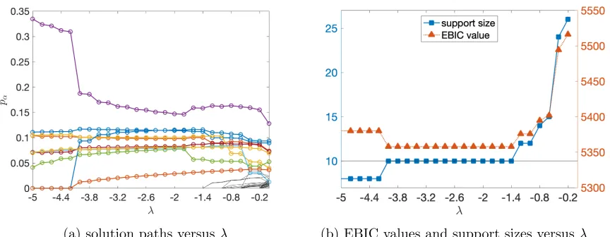
Example 7 Figure 3 presents an illustration of the solution paths of the estimated propor-tions versus λ based on a simulated dataset with N = 150, K = 10, and J = 30. The Q-matrixQ= (Q>1, Q2>, Q>3)> withQi in the following form,
Q1=
1 0 . .. . .. 0 1
, Q2=
1 1 0
. .. . .. . .. 1
0 1
, Q3=
1 1 0
1 . .. . .. . .. . .. 1
0 1 1
. (22)
When generating the data, 10 attribute patterns are randomly selected from the 210= 1024
possible ones as true patterns, and the proportion of each of them is set to be0.1. The item parameters are set to 1−θj+ =θ−j = 0.2 for each j under a two-parameter SLAM. In the current setting with K = 10, we take the set of patterns as input to the PEM algorithm to be Ainput = {0,1}K. Figure 3(a) plots the solution paths of the estimated proportions
of all the 210 = 1024 attribute patterns as λ varies in {−0.2,−0.4,· · · ,−4.8,−5.0}. The 10 true attribute patterns are plotted with colored lines with circles while the remaining
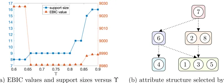
210−10 attribute patterns are plotted with black solid lines. Figure 3(b) plots the estimated support size of p versus λ, and the EBIC value versus λ. We observe that when λ ∈
simulation results which show that the proposed methods combined with EBIC indeed have good performance in general.
(a) solution paths versus λ (b) EBIC values and support sizes versusλ
Figure 3: PEM solution paths and EBIC values in one trial,N = 150.
4.1.2. Variational EM algorithm from an alternative formulation.
In the following, we discuss an alternative formulation of the objective function (17) and propose a variational EM algorithm for estimation, by treating the proportion parameters p as latent random variables. As discussed in Remark 12, for the objective function (17) with λ∈ (−∞,−1], the penalty term Q2K
l=1pλαl does not correspond to a proper Dirichlet distribution density. However, for any arbitrarily smallλvalue, the objective function (17) can be replaced by the following alternative formulation:
`λ,pseudoΥ (Θ,p) = Υ·`(Θ,p) + (β−1) X
α∈Ainput
logρ
N(pα) forβ ∈(0,1), Υ∈(0,1]. (23)
where we introduce a new parameter Υ∈(0,1] and replaceλwithβ−1 to respect the con-vectional notation of a Dirichlet distribution with hyperparameter β ∈(0,1) to encourage sparsity. Withβ ∈(0,1) and Υ∈(0,1], the ratio (1−β)/Υ can be arbitrarily large when Υ is arbitrarily close to zero, therefore making (23) equivalent to (17).
(2016) and Holmes and Walker (2017) for Bayesian learning under model misspecification, and Yang et al. (2019) and Ch´erief-Abdellatif and Alquier (2018) for variational Bayesian inference. Different from these works, here we use the alternative formulation (23) of the original objective function (17) in order to consistently select the significant latent attribute patterns.
The formulation (23) allows for a variational EM algorithm for obtaining the item pa-rameters Θ and the posterior means of the latent variables p. Here we treat Θ still as model parameters, then we follow the general derivation of variational algorithms in Blei et al. (2017) to derive Algorithm 2. We denote the digamma function by Ψ(x) = dxd log Γ(x) forx∈(0,∞). In particular, the complete log likelihood is
`λ,compΥ (Θ| R,A,p) = X
α∈Ainput n
Υ·h X
i
I(Ai=α)
i
+β−1
o
logρN(pα) (24)
+ Υ·n X
α∈Ainput X
i
I(Ai =α)
X
j
h
Ri,jlog(θj,α) + (1−Ri,j) log(1−θj,α)
io .
In the variational E step, we first obtain the conditional probability ofI(Ai =αl) for each
individualiand each input attribute patternαl, which we denote byϕi,αl. In updating this
ϕi,αl, the variational posterior distribution of the pα’s are used, which is still a Dirichlet distribution with mean parameters (∆1, . . . ,∆|Ainput|) updated in the previous E step (or
from initializations if in the first iteration). Then we update the mean parameters for the variational posterior distribution of pαl’s based on the obtained ϕi,αl, following the conventional derivation in variational inference. After finishing this E step, in the M step we maximize the complete likelihood with respect to Θ, by substituting the I(Ai = αl)’s
withϕi,αl’s. Note that taking the derivatives of (24) with respect toθj,αl’s does not involve either terms ofpαl or terms of Υ andβ, so only ϕi,αl are used in the M step for updating
Θ. Indeed, the M step of updating Θ in the current Algorithm 2 takes the same form as that of Algorithm 1.
Similar to Algorithm 1, in the practical use of Algorithm 2 for pattern selection, we recommend using a sequential fitting procedure. For a small fixed β > 0, we choose a sequence of Υ values 1>Υ1 >Υ2 >· · ·>ΥB >0 where Υ1 should be close to 1 and ΥB
should be relatively small. In our simulation studies, we found a ΥB = 0.3 is sufficient in
most of cases. Then we sequentially run Algorithm 2 for B times with fractional powers Υ1, . . . ,ΥB respectively and use estimated parameters from FP-VEM with Υb as initial
values for FP-VEM with Υb+1. In the end, we also use EBIC to select the best Υ. Sinceβ
and Υ can be viewed as acting together through the term (1−β)/Υ, in terms of practical parameter tuning, we recommend fixing β to a relatively small value, say β = 0.01, and let the fractional power Υ ∈ (0,1] vary to control the sparsity level of the proportion parameters.
4.2. Screening as a preprocessing step when 2K N
Algorithm 2:FP-VEM: Fractional Power Variational EM for Υ∈(0,1]
Data: Q,R, and candidate attribute patternsAinput.
Initialize ∆= (∆(0)1 , . . . ,∆(0)|A
input|) = (β, . . . , β). while not converged do
In the (t+ 1)th iteration,
for(i, l)∈[N]×[|Ainput|]do
ϕ(i,αt+1)
l =
expnΨ(∆(lt)) + Υ·P
j
h
Ri,jlog(θ(j,αt)l) + (1−Ri,j) log(1−θ
(t)
j,αl)
io
P
mexp
n
Ψ(∆(mt)) + Υ·Pj
h
Ri,jlog(θj,α(t)m) + (1−Ri,j) log(1−θ
(t)
j,αm)
io;
forl∈[|Ainput|]do
∆(lt+1)←β+ Υ×PN
i=1ϕ (t+1)
i,l ;
forj∈[J]do Θ(t+1)=
arg maxΘ nP
αl
P
iϕ
(t+1)
i,αl
P
j
h
Ri,jlog(θj,αl) + (1−Ri,j) log(1−θj,αl)
io
After the totalT iterations,
for αl∈ Ainput do pαl ←∆
(T)
l /(
P
m∆
(T)
m ).
output:{αl∈ Ainput: pαl > ρN}.
bring down the number of candidate attribute patterns, and then perform the shrinkage estimation.
We next describe our screening approach. Recall that for each subject i = 1, . . . , N, we denote his/her latent attribute pattern by Ai = (Ai,1, . . . , Ai,K) ∈ {0,1}K. In the
screening stage we jointly estimate the item parameters Θ and the {Ai, i ∈ [N]} to get
a rough estimation of each subject i’s attribute pattern, and gather all the N estimated attribute profiles as candidate patterns. The estimation ofpis postponed to the estimation stage. Under the basic two-parameter SLAM, the complete log likelihood involving the latent variables {Ai, i∈[N]} takes the form
`complete(Θ,A) =
N X i=1 J X j=1 h Ri,j Y k
Aqi,kj,klogθj++ (1−Y
k
Aqi,kj,k) logθ−j i
+ (1−Ri,j)
Y
k
Aqj,k
i,k log(1−θ
+
j ) + (1−
Y
k
Aqj,k
i,k ) log(1−θ − j )
i .
We next derive an algorithm with a stochastic EM flavor to estimate the posterior mean of each latent variableAi,k, denoted by a matrix (bai,k) of sizeN×K, wherebai,k =E[Ai,k |
·
].In the end of the algorithm, we obtain the binary matrix W containing the candidate attribute patterns by definingW = (wi,k)N×Kwithwi,k =I(bai,k >1/2).In such a screening
i’s each single attribute k. This results in fast and valid screening of attribute patterns. Viewing theith row vector ofW as the estimated attribute pattern of subjecti, the unique row vectors inW are the roughly selected attribute patterns output by the screening stage. We denote this set of candidate patterns by Abscreen. As long as the screening has the nice
property of “no false exclusion”, meaning the rows in W contain all the true attribute patterns, then the screening stage is considered successful. The selected candidate patterns are passed along to the shrinkage estimation stage as input patterns.
We say the screening procedure has the sure screening property if asN goes to infinity, the probability of all the true attribute patterns included inAbscreen goes to one. The next
theorem establishes the sure screening property of the proposed screening procedure.
Theorem 17 (sure screening property) Suppose the identifiability conditions in Theo-rem 2 and the constraints (20)are satisfied. The screening procedure applied to a SLAM that covers the two-parameter SLAM as a submodel has the sure screening property. Specifically, there exists a constant βmin >0 such that P(Abscreen⊇ A0)≥1− |A0|exp(−N βmin)→1 as N → ∞.
Theorem 17 shows that the probability of the screening procedure failing to include all true patterns has an exponential decay with the sample size N. We point out that despite having the nice property of sure screening, the screening procedure does not guarantee consistency in selecting exactly the set A0 of true patterns, if the number of observed
variables per subjectJ is not large enough. Generally speaking, asN goes large butJ does not, the setAbscreen will include many false attribute patterns, although it will contain the
true set A0 with probability tending to one. Therefore the shrinkage estimation approach
in Section 4.1 is still essential to performing pattern selection.
In Algorithm 3, we present the proposed screening algorithm with stochastic approxi-mations based on a number ofMeffGibbs samples ofAin the E step. Alternatively, we can
also use an even faster screening procedure by just updating the conditional probability of each subject possessing each attribute (i.e., the conditional posterior mean of each Ai,k) in
each E step, conditioning on everything else; we term this alternative procedure the varia-tional screening procedure. As stated before, the screening algorithm is derived based on the log-likelihood of the two-parameter SLAM, but can be applied to a multi-parameter SLAM that covers the two-parameter SLAM as a submodel. After the screening stage, the set of attribute patterns as input to the shrinkage Algorithms 1 or 2 is taken asAinput=Abscreen.
Screening drastically lowers down the computational cost of the subsequent shrinkage es-timation, and the number of candidate patterns fed to the shrinkage stage is kept at the order ofN, even if the original number of possible configurations 2KN.