Binomial Option Pricing Model
by
ODEGBILE, Olufemi Olusola
African Institute for Mathematical Sciences 6 Melrose Road,
Muizenberg, 7945 Cape Town South Africa
[email protected], [email protected]
Supervisor:
Professor Jean-Claude Ndogmo
University of the Western Cape Department of Mathematics
Private Bag X17 Bellville 7535 Republic of South Africa
Contents
List of Figures iii
Abstract iv
Acknowledgements v
1 Introduction 1
1.1 Option Contracts . . . 3
1.2 Underlying Assets . . . 4
1.3 Payoff of Option Contracts . . . 5
2 Binomial Option Pricing (BOP) Model 8
2.1 Pricing Option Contracts Via Arbitrage . . . 8
2.2 Single-Period BOP Model on a Non-Dividend-Paying Stock . . . 12
2.3 Multiperiod BOP Model on a Non-Dividend-Paying Stock . . . 16
3 BOP and Black-Scholes Models 21
3.1 Convergence of the BOP Model to the Black-Scholes Model . . . 21
3.2 Numerical Method . . . 27
3.3 Conclusion . . . 27
B BOP Model’s Convergence for a European Put Option (Python Codes) 34
C BOP Model’s Convergence for an American Call Option (Python Codes) 36
D BOP Model’s Convergence for an American Put Option (Python Codes) 38
List of Figures
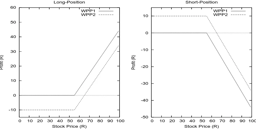
1.1 Profit profile (in rand) of a European call option on one Cisco share. Premium=R10; Strike
price=R55. WPP1 and WPP2 denote Without-Premium-Paid and With-Premium-Paid respectively. 6
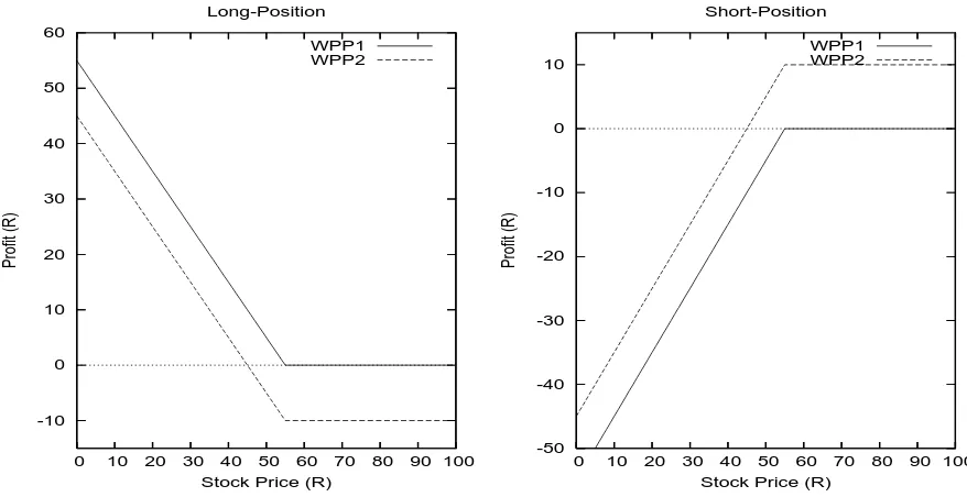
1.2 Profit profile (in rand) of a European put option on one Cisco share. Premium=R10; Strike price=R55. WPP1 and WPP2 denote Without-Premium-Paid and With-Premium-Paid respectively. 7
2.1 (A). One-period BOP model for stock price; (B). Value of one-period call in BOP model . . . 13 2.2 (A). Two-period BOP model for stock price; (B). Value of two-period call in BOP model . . . . 16 2.3 An example to illustrate the dynamism of hedge ratio. (A). Two-period BOP model for stock price;
(B). Value of two-period call in BOP model . . . 17 3.1 Convergence of BOP model of a European call option. The parameters used areS= 100,X= 100,
r= 0.08,σ= 0.2 andt= 1. The analytical values given by Black-Scholes formula is 12.1106. . . . 29
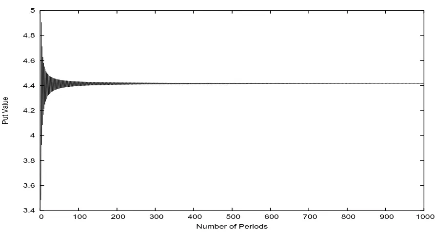
3.2 Convergence of BOP model of a European put option. The parameters used areS= 100,X= 100,
r= 0.08,σ= 0.2 andt= 1. The analytical values given by Black-Scholes formula is 4.4223. . . 29
3.3 BOP model of an American call option. The parameters used are S = 100, X = 100,r = 0.08,
σ= 0.2 andt= 1. . . . 30
3.4 BOP model of an American put option. The parameters used are S = 100, X = 100,r = 0.08,
Abstract
Acknowledgements
Unto Him that has made me laugh be all glory forever. I thank the mighty One that has done great things for me.
My profound gratitude goes to my supervisor, Prof. J. C. Ndogmo, for introducing me to a new discipline and Archie, for his sincere advice concerning my essay. I would like to thank the management of AIMS for this wonderful opportunity given to me. I pray that AIMS shall be sustained by His abundant riches in Christ Jesus. I also thank Dr. Mike Pickles for his selfless service and for always being there for us. A glorious future awaits you. All the invited lecturers, teaching staffs and non-teaching staffs are not left out of my appreciation for making AIMS an exciting place to be with all their long mails, “Think about it.”, “What do you think?”, “Work hard”, “Figure it out.” and “Does that make sense?”.
More so, I am grateful to my father-in-the-Lord, Pastor Omololu Adegoke, and all the member of TLR for lifting me up always in the place of prayer. My gratitude also goes to the entire members of RCCG, victory centre, the Friendship Bible Coffees and my fellowship group at AIMS for creating an atmosphere for me both to serve God and excel in my academics. I pray that none of us shall be disobedient to the heavenly vision.
I would also like to appreciate entire member of “G8” for being right people to mix with. I am blessed to know you all. They are Bolaji, Isaac, Naziga, Doom-Null, Gideon, Henry, and Okeke. May our dreams and our hope for the world to come and this world be materialised. I am also grateful to Yemi Ajibesin , Richard Akinola, all AIMS students, and well wishers, for their good counsel, support, and helping hands.
That no words of appreciation is enough to commensurate support both spiritually and physically from my parent, Mr. J. O. Odegbile and Mrs. A. B. Odegbile, is not an overstatement. I thank God for having someone like you. I would equally like to appreciate the keen support of my loving and caring brother and sisters. They are Kayode, Folake, Omolara, and Olaitan. May we live to see the goodness of the Lord in the land of the living.
Chapter 1
Introduction
The wordderivative originates from mathematics and refers to a variable, which has been derived from another variable. Derivatives are so called because they have no value of their own. They derive there values from the values of some other assets, which is known as the underlying. Ex-amples of derivatives are forward contracts, future contracts and option contracts. The history of derivatives is quite colourful and surprisingly longer than most people think. The first exchange for trading derivatives appears to have been the Royal Exchange in London, which permitted forward contracting [3]. The celebrated Dutch Tulip bulb mania was characterised by forward contracting on tulip bulbs around 1637 (see [15]). The first future contracts are generally traced to the Yodoya rice market in Osaka, Japan around 1650. These were evidently standardised contracts, which made them much like today’s futures, although it is not known if the contracts were marked to market daily and/or had credit guarantees [3].
The primary objectives of any investor are to maximise returns and minimise risks. Derivatives are contracts that originated from the need to minimise risk. This is evident in the motivation behind the creation of the Chicago Board of Trade (CBOT) in 1848, which is currently the largest derivative exchange in the world [3]. Due to its prime location on Lake Michigan, Chicago was developing as a major centre for the storage, sale, and distribution of Midwestern grain. Also due to the seasonality of grain, however, Chicago’s storage facilities were unable to accommodate the enormous increase in supply that occurred following the harvest. Similarly, its facilities were underutilised in the spring. Chicago spot prices rose and fell drastically. A group of grain traders created the ”to-arrive” contract, which permitted farmers to lock in the price and deliver the grain later. This allowed the farmer to store the grain either on the farm or at a storage facility nearby and deliver it to Chicago months later. These to-arrive contracts proved useful as a device for hedging and speculating on price changes. These contracts were eventually standardised around 1865, and in 1925 the first futures clearinghouse was formed.
the principle of put-call parity. Sage would buy the stock and a put from his customer and sell the customer a call. By fixing the put, call, and strike prices, Sage was creating a synthetic loan with an interest rate significantly higher than usury laws allowed. More so, derivatives have had a long presence in India. The commodity derivative market has been functioning in India since the nineteenth century with organised trading in cotton through the establishment of Cotton Trade Association in 1875. Since then contracts on various other commodities have been introduced as well. In 1874 the Chicago Mercantile Exchanges predecessor, the Chicago Produce Exchange, was formed. It became the modern day Merc in 1919. Other exchanges had been popping up around the world, especially in Africa, and continue to do so.
1973 marked the creation of both the Chicago Board Options Exchange and the publication of perhaps the most famous formula in finance, the option pricing model of Fischer Black and Myron Scholes [2]. These events revolutionised the investment world in ways no one could imagine at that time. The Black-Scholes model, as it came to be known, set up a mathematical framework that formed the basis for an explosive revolution in the use of derivatives. The 1980s marked the beginning of the era of swaps and other over-the-counter derivatives. Although over-the-counter options and forwards had previously existed, the generation of corporate financial managers of that decade was the first to come out of business schools with exposure to derivatives. Soon virtually every large corporation, and even some that were not so large, were using derivatives to hedge, and in some cases, speculate on interest rate, exchange rate and commodity risk. New products were rapidly created to hedge the now-recognised wide varieties of risks so that, at the end of 1999, U.S. commercial banks, the leading players in global derivatives markets, reported outstanding derivatives contracts with a notional value of $33 trillion [8]. As the problems became more complex, Wall Street turned increasingly to the talents of mathematicians and physicists, offering them new and quite different career paths and unheard-of money. The instruments became more complex and were sometimes even referred to as exotic.
1.1
Option Contracts
Option contracts are contracts that convey upon the holder the right to buy or sell an asset at a certain future time, at a fixed price. The fixed future time and price are respectively called the
expiration date, or maturity and the exercise, or strike price. Options can be grouped into two main categories depending on whether the holder’s right is to buy (this is called a call option) or to sell (this is called aput option). The holder is not obliged to exercise the right at the maturity. The right is only exercised if it is economically advantageous and whenever this is done, the other party is obliged to honour the contract. Options that can be exercised only at maturity are called
European options while those that can be exercised at any time up to maturity are calledAmerican options. The names of these options do not imply any geographical limitation to where they are being traded since both European and American options are traded in America, Europe, and some other places of the world. Clearly, the American option has the benefits of the European option but not vice versa, and so, it can not cost less than its European counterpart with the same parameters.
In any option contract, there are two parties involved. An investor that buys an option (that is, an option’s holder) and an investor that sells an option (that is, an option’s writer). The option’s holder is said to take along position while the option’s writer is said to take ashort position. Detail about the payoff associated to each position shall be discussed in the last section of this chapter. Before then, it should be noted that there are basically four types of option positions. They are the following [11]: (1) a long position in a call option, (2) a long position in a put option, (3) a short position in a call option and, (4) a short position in a put option.
Furthermore, options can be traded on an exchange or in the over-the-counter market. An ex-change is a market where individuals trade standardised contracts. That is, an orderly market with well-defined contracts. Example of exchanges are American Stock Exchange (AEX), Chicago Board Options Exchange (CBOE), London International Financial Futures and Options Exchange (LIFFE), Osaka Securities Exchange (OSA), Johannesburg Stock Exchange (JSE) etc [11]. A key advantage of exchange-traded options is that there is a guarantee that the terms of the contracts will be honoured especially by the help of the clearing house. Alternatively, trades are done over the phone and are usually between a financial institutions and one of its corporate client in over-the-counter market (OTC). A major advantage of OTC is that the market participants are free to negotiate any mutually attractive deal. A major setback is that there is a small risk that the contract will not be honoured.
In summary, an option contract is uniquely described by the following specifications ([12] and [17]):
• The option type: call or put.
• The description of the underlying asset.
• The maturity, exercise price, and how the delivery is to be carried out.
• The rule for the exercise: European or American.
1.2
Underlying Assets
Options can be traded on a wide range of commodities and financial assets. The commodities include wool, corn, wheat, sugar, tin, petroleum, gold etc. and the financial assets include stocks, currencies, and treasury bonds [11]. Exchange-traded options are currently actively traded on stocks, stock indices, foreign currencies, and futures contracts [11].
Stock Options
Exchanges trading stock options are ASE, CBOE, LIFFE among others. In America, and in many other exchanges including JSE, options are traded on numerous stocks, more than 500 different stocks in fact [11]. The options are standardised in such a way that an option contract consists of 100 shares. Example is IBM July 125 call. This is an option contract that gives a right to buy 100 IBM’s shares at a strike price of $125 each in three months time [17].
Foreign Exchange Options
This contract gives the holder the right to buy or sell a specific foreign currency at a fixed future time at a fixed price. The size of this contract generally depends on the foreign currency in question. Foreign currency options are important tools in hedging risk, and it can be traded as either an American or a European option [11].
Index Options
This has the same standardised size as a stock option. One contract is to buy or sell 100 times the index at a specified strike price. An example of this type of option contract is a call contract on the S&P 100 with a strike price of 980. If the option is exercised, the sum of money equivalent to the payoff of the option is given to the holder of the option.
Futures Options
1.3
Payoff of Option Contracts
In this section, we shall be concerned with what the two parties involved in an option contract realise at maturity. In this work, unless otherwise stated, the underlying asset is a stock.
Let ST be the stock price at the expiration time T and X the strike price. Then the payoff, say Qc, of a European call option is
Qc =max(ST −X,0) (1.1)
This reflects the fact that an option might be exercised if ST > X and might not be exercised if ST ≤X. The payoff from a call option results in a loss on the short position, and a gain on the long position, when it is exercised. The payoff, say Qp, of a European put option is
Qp =max(X−ST,0) (1.2)
Similarly, this reflects the fact that an option might be exercised if ST < X and might not be exercised if ST ≥ X. Also, the payoff from a put option results in a loss on the short position, and a gain on the long position, when it is exercised. This implies that, in term of the payoff, the option’s writer realises nothing but a loss and the option’s holder has nothing to loose, as it does not take into account any initial commitment from his part.
So, no reasonable person is expected to take up a short position in an option contract without any compensation. This is a problem since one party cannot make up a contract. To this end, it is demanded that the holder of a long position in an option contract should pay the other party some amount to acquire the rights granted under an option contract. The sum paid is called theoption price or premium. So, premium is what an option is worth at the beginning of the contract. This essay is concerned with the determination of a fair price for an option such that riskless profit is ruled out. This shall be dealt with in detail in the remaining chapters. Figures 1.1 and 1.2 are profit profiles of European call and put options, respectively. An option should be exercised as it has some values at expiry, for this will reduce the net loss. If we definex+ as follows:
x+=
(
x ifx >0, 0 ifx≤0,
equations (1.1) and (1.2) become
(ST −X)+ (1.3)
and
(X−ST)+, (1.4)
respectively. These are the forms in which we shall be writing option payoff in subsequent chapters.
Intrinsic and Time Values: TheIntrinsic value of an option is the value realised on an option if it were to be exercised immediately while the time value of an option is the value of an option arising from the time left to maturity. Since an option is usually worth at least its intrinsic value at any time, intrinsic value is the minimum premium that an option may be worth. So, whenever an option has time remaining to its maturity, its total price consists of its intrinsic value plus its time value.
-10 0 10 20 30 40 50 60
0 10 20 30 40 50 60 70 80 90 100
Profit (R)
Stock Price (R) Long-Position
WPP1 WPP2
-50 -40 -30 -20 -10 0 10
0 10 20 30 40 50 60 70 80 90 100
Profit (R)
Stock Price (R) Short-Position
[image:12.595.86.525.206.430.2]WPP1 WPP2
Figure 1.1: Profit profile (in rand) of a European call option on one Cisco share. Premium=R10; Strike price=R55. WPP1 and WPP2 denote Without-Premium-Paid and With-Premium-Paid respectively.
In-, At-, Out-Of-The-Money: A call (pull) option is said to be in-the-money if the asset price is more (less) than the strike price, while it is out-of-the-money if the asset price is less (more) than the strike price. More so, an option is at-the-money if the strike price equals the price of the underlying asset.
A premium is dependent on certain properties of both the underlying asset and the terms of the option. The major quantifiable factors influencing an option price are the following ([17] and [7]):
• Price of the underlying stock.
• Striking price of the option itself.
• Time remaining until maturity.
• Volatility of the underlying stock: Volatilityis the measure of uncertainty about the evolution of the price of the underlying stock
-10 0 10 20 30 40 50 60
0 10 20 30 40 50 60 70 80 90 100
Profit (R)
Stock Price (R) Long-Position
WPP1 WPP2
-50 -40 -30 -20 -10 0 10
0 10 20 30 40 50 60 70 80 90 100
Profit (R)
Stock Price (R) Short-Position
[image:13.595.84.523.101.327.2]WPP1 WPP2
Figure 1.2: Profit profile (in rand) of a European put option on one Cisco share. Premium=R10; Strike price=R55. WPP1 and WPP2 denote Without-Premium-Paid and With-Premium-Paid respectively.
• Dividend rate and policy of the underlying stock.
Chapter 2
Binomial Option Pricing (BOP)
Model
The binomial model is a discrete-time model for pricing option in which it is assumed that price change in the underlying asset occur only after regular time interval. It involves constructing a tree which represents different possible paths that the price of the underlying asset might follow. This tree is called the Binomial Tree. This model is based on an assumption about the evolution of the price of the underlying asset and the so called ’no-arbitrage principle’. That is, the BOP model determines an option price that does not permit arbitrage opportunities. The justification of this principle lies in the fact that in the presence of the possibility to make gains without risk, all investors that are faced with such possibility will try to realise it. Thanks to the law of supply and demand, this would result in an immediate adjustment of prices in the market such that arbitrage opportunity will disappear. We shall start by introducing this general principle by a concrete example and then examine its immediate consequences. After this, we shall look in detail at the one-period BOP model, which is then generalised ton number of periods in the last section.
2.1
Pricing Option Contracts Via Arbitrage
Suppose that the risk free continuously compounded interest rate isr. Let the price of a stock (in rand) be 200 per share and suppose we know that, after one year, its price will be either 400 or 100. Suppose further that, the strike price of a European call option on the stock that matures after one year is 300. Then, the return from the option contract at maturity is
return =
(
Our aim is to calculate the option price such that there exists no arbitrage opportunity, that is, no sure-win, riskless or guarantee profit without initial capital. We shall achieve this by building up a portfolio that replicates the option’s return at maturity. The portfolio is a loan of 100e−ry amount
and a cash of (200−100e−r)y amount from our pocket. This enables us to purchase y shares of
the stock. Then, at maturity, the payoff of the portfolio after we have paid back the loan with an interest is
payoff =
(
300y if the stock price is 400, 0 if the stock price is 100.
Therefore, to replicate the option’s return at maturity, we should have y = 1/3. Thus, by pay-ing (200−100e−ry) and borrowing 100e−ry to buy 1/3 share of the stock, we can replicate the
option’s return at the maturity. These two investment are identical, so their cost must also be the same to avoid an arbitrage opportunity. To illustrate this, suppose that c is the option price. Then, if c > (200−100e−r)/3, there is an arbitrage gain by using our funding along with the
borrowed money to buy 1/3 share of the stock while simultaneously selling one option contract. This leads to an arbitrage gain of at least ((3c−200)er+ 100)/3 amount. On the other hand, if c < (200−100e−r)/3, there is also an arbitrage gain by selling short 1/3 share of the stock and
buying one option contract while simultaneously depositing (200−3c)/3 in a bank. Byshort selling
a risky asset like stock, we mean that an investor borrows the stock, sells it, and uses the proceed to make some other investments and then repurchase the stock and return it to the owner with any dividends due [16]. This strategy makes sense sincec <(200−100e−r)/3 implies that
0< 100 3 e
−r < 200
3 −c which is equivalent to 0< 100
3 <( 200
3 −c)e r.
Then, there is an arbitrage gain of
(200 3 −c)e
r −100
3 (2.1)
amount, if the stock price is 100. However, if the stock price is 400, the net amount we owe is
400
3 −
100
3 =
100 3 <(
200 3 −c)e
r.
And so, the arbitrage profit is also given by equation (2.1).
So far, the principle we have used to determine the option price is called ’pricing via arbitrage’. What follow are the consequences of this principle:
Proposition 2.1.1 (1) Letcbe the price of a European call option to purchase a security whose present price is S. Then 0≤c≤S.
(2) Let p be the price of a European put option to sell a security whose present price is S for the amount X. Then 0≤p≤X
Proposition 2.1.2 [13] (1) For the price c of a European call option, with strike price X ≥0
and expiration date t, we have
(S−Xe−rt)+≤c≤S, (2.2)
where S is the present price of the underlying security.
(2) For the price p of a European put option, with strike price X ≥ 0 and expiration date t, we have
(Xe−rt−S)+
≤p≤X, (2.3)
where S is the present price of the underlying security.
Proof. (1) Due to Proposition 2.1.1, we have that the inequality c≤S holds. Now, suppose that
c <(S−Xe−rt)+, (2.4)
where due to non-negativity of a call option, equation (2.4) implies that we must have
(S−Xe−rt)+
=S−Xe−rt which is implies that (S−c)ert> X. (2.5)
Then, there exits an arbitrage opportunity by short selling one share of the security and buying one call option on the security while simultaneously depositing S−c in a bank. At time t, we return the security back by buying the security at the cost equal to the minimum of X and the market price of the security. We also realise (S−c)ert from the amount deposited in the bank. Hence, this transaction yields at least
(S−c)ert−X >0
as an arbitrage gain.
(2) Similarly, due to Proposition 2.1.1, we have that the inequality p ≤ X holds. Now, suppose that
p <(Xe−rt−S)+, (2.6)
where due to non-negativity of a put option, equation (2.6) implies that we must have
(Xe−rt−S)+=Xe−rt−S which is implies that (S+p)ert< X. (2.7)
An arbitrage opportunity also exits by borrowingS+p from a bank and using it to buy one share of the security and one put option on the security. At time t, we realise an arbitrage gain of at least
X−(S+p)ert>0
amount after we have paid back (S+p)ert amount to the bank and sold the security back at
Theorem 2.1.1 [13] (Put-Call Parity for European Options)
For the prices c and p of respective European call and put options with the same exercise time t and the same strike price X ≥0 on the same asset, we have
c+Xe−rt =p+S (2.8)
where S is the present price of the underlying security.
Proof. Suppose that eitherS+p−c < Xe−rt orS+p−c > Xe−rt.
If S+p−c < Xe−rt, equivalently, we have that (S+p−c)ert < X. Then, there is an arbitrage
opportunity by borrowingS+p−c amount from a bank and simultaneously buying one share of the security and one put option on the security while selling one call option on the security. At timet, the return on the portfolio is
St+ (X−St)+−(St−X)+.
Since
St+ (X−St)+−(St−X)+ =
(
X if St> X, X if St< X,
there is an arbitrage gain of
X−(S+p−c)ert>0
after we have paid back the loan with an interest. If S+p−c > Xe−rt, there is also an arbitrage
opportunity by selling short one share of the security and selling the put option while simultaneously buying on call option on the security and depositing the net amount ofS+p−cin a bank. Similarly, at timet, the return on the portfolio is
(St−X)+−(X−St)+−St.
Since
(St−X)+−(X−St)+−St=
(
−X ifSt> X, −X ifSt< X,
it implies that we oweX amount at timet. Then, there is an arbitrage gain of
(S+p−c)ert−X >0,
amount after we have withdrawn the deposit with an interest from the bank.
1. Proposition 2.1.2 gives both the upper and lower bounds of the European call and put options. These bounds are called arbitrage bounds.
2. Since an American option enjoys the privilledges granted by a European option, C ≥c and P ≥ p [13]. More so, because of the early exercise opportunity under American options, arbitrage bounds are the following [11]:
(S−X)+
≤C ≤S and (X−S)+
≤P ≤X.
3. Ifr >0, it is never optimal to exercise an American call option on a non-dividend paying stock before its expiration ([13] and [18]). Furthermore, put-call parity holds only for European options an analogue to put-call parity for American option calls and puts is ([11] and [13])
S−X ≤C−P ≤S−Xe−rt. (2.9)
4. All the results produced so far in this section have assumed that we are dealing with non-dividend-paying stock. Suppose that D is the present value of the dividends during the life time of the option. Effects of dividends are highlighted below.
For a European option, we have [11]
(S−Xe−rt−D)+
≤c≤S and (D+Xe−rt−S)+
≤p≤X.
The put-call parity also becomes [11]
c+D+Xe−rt=p+S.
In case of an American option, we have [11]
(S−X−D)+ ≤C≤S and (D+X−S)+≤P ≤X
and equation (2.9) also becomes [11]
S−D−X ≤C−P ≤S−Xe−rt.
2.2
Single-Period BOP Model on a Non-Dividend-Paying Stock
In the BOP model, time is discrete and measured in periods. The model assumes that the stock priceS at the beginning of a period can either go touS ordS with
S
dS
Cu = (uS−X)+ uS
c
Cd= (dS−X)+
[image:19.595.163.518.116.322.2](A) (B)
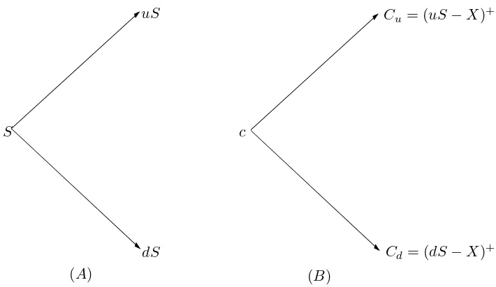
Figure 2.1: (A). One-period BOP model for stock price; (B). Value of one-period call in BOP model
r is the risk free continuously compounded interest rate, T is the maturity,and n is the number of periods before the maturity. More precisely, in case d ≥erδt, financing a stock investment via credit results in an arbitrage gain. In the case ofu≤erδt, selling a stock short and depositing the profit in a bank constitutes an arbitrage gain. Now, suppose that the maturity of a European call option on a stock that is presently sellingS, with a strike price of X is only one period from now (see Figure 2.1). Suppose further that we set up a portfolio by borrowing B from a bank and put up from our own fund to buy ∆ shares of the stock. We call ∆ thehedge ratio ordelta. This costs ∆S−B. LetCu be the option’s return if the price moves to uS and Cd be the option’s return if the price moves to dS at the maturity. Clearly,
Cu = (uS−X)+ and Cd= (dS−X)+.
Then, we choose ∆ andB such that the portfolio replicates option’s return at maturity:
∆uS−erδtB =Cu,
∆dS−erδtB=Cd.
By solving the two equations simultaneously, we obtain
∆ = Cu−Cd
S(u−d) ≥0 and B =
dCu−uCd u−d e
This implies that
∆S−B = (e rδt
−d)Cu+ (u−erδt)Cd erδt(u−d) ≥0,
sinced < erδt< u. These two investment are identical, so their cost must also be the same to avoid any arbitrage opportunity. In fact, suppose that the option price bec. Ifc >∆S−B, then there is an arbitrage gain of (c−∆S+B)erδt amount by using our money along with the borrowed money ofB amount to buy ∆ shares of the stock while simultaneously selling one option contract. On the other hand, ifc <∆S−B, equivalentlyerδtB <(∆S
−c)erδt. Then, there is also an arbitrage gain of (∆S−c−B)erδt amount by selling short ∆ shares of the stock and buying one option contract while simultaneously depositing ∆S−c in a bank since
∆uS−Cu= ∆dS−Cd=erδtB <(∆S−c)erδt.
Thus, to avoid any arbitrage opportunity, we must havec= ∆S−B. Hence,
c= (e rδt
−d)Cu+ (u−erδt)Cd
erδt(u−d) . (2.10)
A European put option can be similarly priced. This is done by setting up a portfolio by short selling ∆ shares of the stock and putting from our own fund to depositB amount in a Bank. This portfolio costs B−∆S. By carrying out similar analysis as in the European call option’s case, we have the following suitable values for ∆ and B:
∆ = Pd−Pu
S(u−d) ≥0 and B =
uPd−dPu erδt(u−d) ≥0,
wherePd= (X−dS)+
and Pu = (X−uS)+
. This implies that
B−∆S = (e rδt
−d)Pu+ (u−erδt)Pd erδt(u−d) ≥0,
sinced < erδt < u. Consequently, by no-arbitrage principle, the European put option price, sayp, isB−∆S. Hence,
p= (e rδt
−d)Pu+ (u−erδt)Pd
erδt(u−d) . (2.11)
magnitudes of which the investors must agree on. Now rearranging equation (2.10), we have
c =
erδt
−d
u−d
Cu+u−erδt
u−d
Cd
erδt
= pCu+ (1−p)Cd erδt ,
where p=(erδt−d)/(u−d). As 0 < p < 1, if we assume that it is the probability that the stock price will be equal touS, then we have
E[Sδt] = puSδt+ (1−p)dSδt
= (erδt−d)Sδt+dSδt
= erδtSδt
This implies that we are assuming the risk-neutral world when we set the probability of an upward movement of the stock price to bep . For this reason, p is called the risk-neutral probability. The findings above are summarised below.
Proposition 2.2.1 [14] The value of an option equals the expected present value payoff dis-counted at expiration in a risk neutral economy.
The following definition shall be needed shortly:
1. The binomial distribution with parameters nand p is given by
b(j;n, p) =
n j
pj(1−p)n−j.
2. The complementary binomial distribution function with parametersn and pis
Φ(k;n, p)≡ n
X
j=k
b(j;n, p).
Proposition 2.2.2 [14] If Φ(k;n, p) is the complementary binomial distribution function with parameter n andp, then
1−Φ(k;n, p) = Φ(n−k+ 1;n,1−p).
fewer than k heads. Equivalently, 1−Φ(k;n, p) is the same as the probability of getting at least n−k+ 1 tails. Hence,
1−Φ(k;n, p) = k−1
X j=0 n j
pj(1−p)n−j
= n
X
j=n−k+1
n j
(1−p)jpn−j
= Φ(n−k+ 1;n,1−p)
2.3
Multiperiod BOP Model on a Non-Dividend-Paying Stock
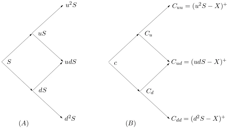
We start by considering the two-period case and then generalise it later in the section. To this end, suppose that we are considering a European call option. Under the two-period binomial tree (see figure 2.2), there are three possible prices at the second period. They areu2
S,udS and d2 S. Let the respective option value at the three prices beCuu,Cud and Cdd. Thus,
Cuu= (u2
S−X)+
, Cud = (udS−X)+
, and Cdd= (d2
S−X)+ .
Since at any node the next two stock prices depend only on the current stock price and not on
S
u2S
Cuu= (u2
S−X)+
uS
c
Cd
(A) (B)
udS
dS
d2 S
Cu
Cud = (udS−X)+
[image:22.595.162.531.473.682.2]Cdd = (d2S−X)+
Figure 2.2: (A). Two-period BOP model for stock price; (B). Value of two-period call in BOP model
So, we obtain the option values at first period by applying the same logic as in BOP model for one period. Then, it follows that
Cu= pCuu+ (1−p)Cud
erδt and Cu=
pCud+ (1−p)Cdd
erδt ,
where p = (erδt
−d)/(u−d). In a similar way, a portfolio can be set up for the call option that costsCu (Cd) if the stock price goes touS (dS, respectively). Thus,
c = pCu+ (1−p)Cd erδt
= p
2
Cuu+ 2p(1−p)Cud+ (1−p)2 Cud e2rδt
= p
2
(u2
S−X)+
+ 2p(1−p)(udS−X)+
+ (1−p)2
(d2
S−X)+
e2rδt .
Hedging ratio ∆ andB at each node can be derived using the same argument. For example, ∆ at Cu and Cd are respectively
Cuu−Cud Suu−Sud and
Cud−Cdd Sud−Sdd.
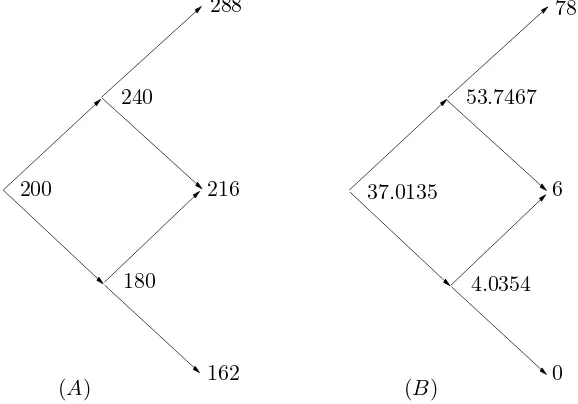
In fact, ∆ changes from one node to another. This dynamism and its consequence are illustrated
200
288 78
240
37.0135
4.0354
(A) (B)
216
180
162
53.7467
6
[image:23.595.163.452.396.598.2]0
Figure 2.3: An example to illustrate the dynamism of hedge ratio. (A). Two-period BOP model for stock price; (B). Value of two-period call in BOP model
in Figure 2.3 which is an example of a two-period stock price movement of a European call option. The initial price is 200, u= 1.2 and d= 0.9. The strike price in two years is 210 and the risk free interest rate is 0.12. Let the respective hedge ratio at C, Cu, and Cd be ∆3, ∆1, and ∆2. Then,
we have the following results:
The implication of this is that 0.8285 share of the stock must be bought at the beginning of the contract. If the stock price moves down, 0.7174 share of the stock must be sold to bring the hedge ratio to 0.1111. On the other hand, if the stock price moves up, additional 0.1715 share of the stock must be bought to bring the hedge ratio to 1.0.
In a similar way, three-period BOP model gives
c = 1
erδt(pCu+ (1−p)Cd)
= 1
e2rδt(p 2
Cuu+ 2p(1−p)Cud+ (1−p)2Cdd)
= 1
e3rδt(p 3
Cuuu+ 3p2(1−p)Cuud+ 3p(1−p)2Cudd+ (1−p)3Cddd)
= 1
e3rδt(p 3
(u3
S−X)+
+ 3p2
(1−p)(u2
dS−X)+
+ 3p(1−p)2
(ud2
S−X)+
+ (1−p)3
(d3
S−X)+
).
Now, we consider the n-period case. By carrying out the same calculation at every node while moving backward in time, we have
c= 1 enrδt n X j=0 n j
pj(1−p)n−j(ujdn−jS−X)+. (2.12)
Similarly, the price of a European put option is
p= 1 enrδt n X j=0 n j
pj(1−p)n−j(X−ujdn−jS)+
. (2.13)
These findings in terms of the complementary distribution function Φ(a;n, p) are summarised below.
Theorem 2.3.1 [5] (Cox-Ross-Rubinstein Formula)
The value of a European call and the value of a European put are
c=SΦ(a;n, p∗ue−rδt)−Xe−nrδtΦ(a;n, p∗), (2.14)
p=Xe−nrδtΦ(n−a+ 1;n,1−p∗)−SΦ(n−a+ 1;n,1−p∗ue−rδt). (2.15)
respectively, where p∗ ≡(erδt−d)/(u−d), a is the minimum number of upward price moves for the option to finish in-the-money, and r is the risk free interest rate.
Proof.
Since ais the minimum number of upward price moves for the option to finish in the money, this implies thatais the smallest non-negative integer such that
Suadn−a≥X, or a=
ln(X/Sdn) ln(u/d)
Obviously,
(ujdn−jS−X)+
=
(
ujdn−jS−X ifj ≥a;
0 otherwise.
Thus,
c = 1
enrδt n
X
j=a
n j
p∗j(1−p∗)n−j(ujdn−jS−X)
= S
n
X
j=a
n j
(p∗ue−rδt)j((1−p∗)de−rδt)n−j−Xe−nrδt
n
X
j=a
n j
p∗j(1−p∗)n−j
= S
n
X
j=a
b(j;n, p∗ue−rδt)−Xe−nrδt
n
X
j=a
b(j;n, p∗)
= SΦ(a;n, p∗ue−rδt)−Xe−nrδtΦ(a;n, p∗),
sincep∗ue−rδt+ (1−p∗)de−rδt= 1.
For the put option, by theorem 2.1.1 we have that
p=Xe−nrδt+c−S.
Substituting in this last equality the expression forc given above, yields
p = SΦ(a;n, p∗ue−rδt)−Xe−nrδtΦ(a;n, p∗) +Xe−nrδt+c−S
= Xe−nrδt(1−Φ(a;n, p∗))−S(1−Φ(a;n, p∗ue−rδt))
Finally, by proposition 2.2.2 we have
p=Xe−nrδtΦ(n−a+ 1;n,1−p∗)−SΦ(n−a+ 1;n,1−p∗ue−rδt)
Remark.
1. The whole discussion about the BOP model started by assuming that prices at each step could only move up or down by pre-determined amounts. While this seems an unrealistic assumption at first; if the steps are made small enough, and if sufficient steps are combined together, the price over an extended period of time can move over almost any possible price path. Thus, this assumption is therefore a reasonable one, provided that the individual steps are small. Another reason that makes the multiperiod assumption reasonable is its convergence. This shall be discussed in detail in the next chapter.
Chapter 3
BOP and Black-Scholes Models
The BOP model converges to the Black-Scholes model when the number of time periods to ex-piration increases to infinity so that, the length of each time period is infinitesimally short. This proof was provided by Cox, Ross, and Rubinstein in 1979 [5]. Their results are derived only for the special case where the up and down factors are given by specific formulas they obtained and that allow the distribution of the stock return to have the same parameters as the desired lognormal distribution in the limit. The Cox, Ross, and Rubinstein proof is elegant but too specific. A more general proof of the convergence of the BOP model to the Black-Scholes model was provided by Hsia [10]. His approach imposes no restrictions on the choice of up and down parameters. In this chapter, we shall employ this approach to prove the convergence. Moreover, we shall end this chapter by a numerical simulation of this convergence.
3.1
Convergence of the BOP Model to the Black-Scholes Model
We start with our ultimate goal, the Black-Scholes formula for a call option. Suppose thatS is the current stock price, X is the strike price, and r is the continuously compounded risk free interest rate. Suppose further thattis the time to expiration andσis the volatility. Then, the Black-Scholes model of a call option on a non-dividend-paying stock is
c = SN(d1)−Xe−rtN(d2) (3.1)
d1 =
ln(S/X) + (r+σ2/2)t
σ√t (3.2)
d2 =
ln(S/X) + (r−σ2/2)t
σ√t =d1−σ √
whereN(di) is the cumulative normal probability fori= 1 and 2 as defined above. Clearly, we are done if we show that
Φ(a;n, pue−rδt)→N(d
1) and Φ(a;n, p)→N(d2),
as n → ∞. To this end, we appeal to the famous DeMoivre-Laplace Limit Theorem (a special case of Central Limit Theorem), which says that a binomial distribution converges to the normal distribution as n → ∞ [9]. For example, for a complementary binomial distribution function Φ(a∗;n, p∗), we have that
Φ(a∗;n, p∗)→
Z ∞
a∗
f(j)dj,
as n → ∞, where j is the binomial random variable with parameters n and p∗ and f(j) is the
density function of a normal distribution. To convert j to a standard normal variable, we define z= (j−E[j])/pVar[j]. Then we would have
Z ∞
a∗
f(j)dj =
Z ∞
z0
f(z)dz,
wherez0 = (a∗−E[j])/
p
Var[j]. This implies that
Φ(a∗;n, p∗)→
Z ∞
z0
f(z)dz= 1−
Z z0
−∞
f(z)dz = 1−N(z0) =N(−z0),
asn→ ∞.
Now, suppose that a random variableYi equals 1 if the price goes up at timeiδtwith probabilityq, and equals 0 if it goes down. Let Stbe the stock price at maturity and j the number of up moves in the firstnperiods. Thenj =Pn
i=1Yi and so,n−j is the number of down moves. The variable Yi is a Bernoulli random variable. Let tbe the time at maturity. Then,
t=nδt or n= t δt.
Hence,St can be expressed as
St=Sujdn−j =dnS
u
d
j
.
This implies that
St S =d
nu d j , and so, ln St S
=jlnu d
+nln(d). (3.4)
Asntends to infinity, there are more and more terms in the summationPn
i=1Yi. SinceY1, ..., Ynis
j=Pn
i=1Yi approaches the normal distribution. Moreover, from equation (3.4)
E[ln(St/S)] = E[j] ln(u/d) +nln(d) (3.5)
and
Var[ln(St/S)] = Var[j](ln(u/d))2. (3.6)
But the Black-Scholes model of option pricing assumes that the stock price behaviour is ageometric Brownian motion [11], that is,
ln
St S
∼N(µt, σ2t),
where µ is the expected rate of return on the stock and σ is the volatility of the stock. So, for the binomial model to converge to the expectation µt and the variance σ2
t of the stock’s true continuously compounded rate of return over the time t, the requirements are the following, as n→ ∞:
E[ln(St/S)]→µt and Var[ln(St/S)]→σ2t.
Then the above requirement can be satisfied by the following values of u,d, and q:
u=eσ
√
δt, d=e−σ√δt and q= 1 2 + 1 2 µ σ r t
n. (3.7)
These are the values ofu and dproposed by Cox, Ross and Rubinstein [5]. Equation (3.7) are not the only values of u, d, and q that satisfy the requirements. The following values also satisfy the same requirements as n→ ∞:
u= exp
"
µt n +σ
r
t n
#
, d= exp
"
µt n −σ
r
t n
#
and q = 1
2 (3.8)
Thus, ln(St/S) approximately becomes a normal variable with meanµtand varianceσ2tasntends to infinity.
Now, equations (3.5) and (3.6) imply that
E[j] = E[ln(St/S)]−nln(d)
ln(u/d) (3.9)
and
Var[j] = Var[ln(St/S)]
(ln(u/d))2 . (3.10)
Recall that the minimum number of upward moves for the option to finish in money is
ln(X/Sdn) ln(u/d)
This implies that
a= ln(X/Sd n)
ln(u/d) +,
where 0≤ <1. Hence, asn→ ∞
Φ(a;n, p∗)→N(α), (3.11)
where
α = −z0 = −
a+ E[j]
p
Var[j]
=
−ln(X/S) +nln(d)−ln(u/d)
ln(u/d) +
E[ln(St/S)]−nln(d) ln(u/d)
, p
Var[ln(St/S)] ln(u/d)
= ln(S/Xp ) + E[ln(St/S)] Var[ln(St/S)] −
ln(u/d)
p
Var[ln(St/S)]
From the properties of the binomial distribution, Var[j] =np∗(1−p∗), wherep∗ is the probability
of success. And so, equation (3.10) implies that
p
Var[ln(St/S)] = ln(u/d)pVar[j] = ln(u/d)pnp∗(1−p∗).
Thus,
α = ln(S/Xp ) + E[ln(St/S)]
Var[ln(St/S)] −
1
p
p∗(1−p∗)
√ n
≈ ln(S/Xp ) + E[ln(St/S)]
Var[ln(St/S)] ,
as n → ∞. Now, we need d to equal d1 and d2 as defined by the Black-Scholes formula when
the probabilities are pue−rδt and p, respectively, where p = (erδt−d)/(u−d). We again appeal
to another famous theorem called Girsanov’s Theorem. The statement of this theorem requires fore knowledge of some definitions and terms and it can be found in [13]. It basically means that whenever we move from a world with one set of risk preferences to a world with another set of risk preferences (in other words, change measure), the expected growth rates in variables change, but their volatilities remain the same [11]. This implies that the volatilities for the two probabilities are the same. So,
α= ln(S/X) + E[ln(St/S)]
σ√t (3.12)
Suppose that the probability of upward moves of stock price sayp∗, ispue−rδt, where
p= (erδt
−d)/(u−d). Then,
erδt=
p∗
u + 1−p∗
d
−1
More so, S/St can be expressed as follows: S St = n Y i=1
(Si−1/Si),
whereS =S0 andSt=Sn. The expectation of this would be
E[S/St] = E[Qni=1(Si−1/Si)] =
n
Y
i=1
E[Si−1/Si],
since each price ratio Si−1/Si is independent of all others. Also, sinceSi =Si−1u with the
proba-bility p∗ andSi =Si
−1dwith the probability 1−p∗,
E[Si−1/Si] = p∗
u + 1−p∗
d .
Thus,
E[S/St] = n
Y
i=1
(p∗(1/u) + (1−p∗)(1/d)) =
p∗
u + 1−p∗
d
n
.
Inverting this and using equation (3.13) gives
(E[S/St])−1 =
p∗
u + 1−p∗
d
−n
=enrδt =ert.
This implies that
ln(E[S/St]) =−rt. (3.14)
Since St/S is lognormally distributed and the inverse of a lognormal distribution is lognormally distributed, S/St is lognormally distributed. Also, for any random variableX that is lognormally distributed, we have the following [18]:
ln(E[X]) = E[ln(X)] + (Var[ln(X)])/2. (3.15)
Equations (3.14) and (3.15) imply that
−rt = E[ln(S/St)] + (Var[ln(S/St)])/2 = E[−ln(St/S)] + (Var[−ln(St/S)])/2
= −E[ln(St/S)] + (Var[ln(St/S)])/2
So,
E[ln(St/S)] =rt+ (Var[ln(St/S)])/2 =rt+ σ2t
2 =
r+σ
2
2
Hence,
α = ln(S/X) + (r+σ
2 /2)t σ√t =d1,
when p∗ =pue−rδt. And so,
Φ(a;n, pue−rδt)→N(d
1),
asn→ ∞.
To prove the convergence of Φ(a;n, p) to N(d2), suppose that p∗ is equal to p, the risk neutral
probability. Then,
erδt=pu+ (1−p)d.
Since Si=Si−1u with the probabilityp andSi =Si−1dwith the probability 1−p,
E[Si/Si−1] =pu+ (1−p)d.
Since
E[St/S] = E[Qn
i=1(Si/Si−1)] =
n
Y
i=1
E[Si/Si−1]
= n
Y
i=1
(pu+ (1−p)d) = (pu+ (1−p)d)n
= enrδt = ert,
it follows that
ln(E[St/S]) =rt. (3.16)
Again, Equations (3.15) and (3.16) imply that
E[ln(St/S)] =rt−(Var[ln(St/S)])/2 =rt− σ2
t
2 =
r−σ 2
2
t.
Hence,
d= ln(S/X) + (r−σ
2 /2)t σ√t =d2,
when p∗ =p. And so,
Φ(a;n, p)→N(d2),
asn→ ∞. Hence, we obtain the convergence of BOP model to Black-Scholes for a European call option.
is, asn→ ∞, a put option price converges to
p = c+Xert−S = SN(d1)−Xe−rtN(d2) +Xert−S
= Xe−rt(1−N(d
2))−S(1−N(d1))
= Xe−rtN(−d2)−SN(−d1).
3.2
Numerical Method
The Black-Scholes model requires five parameters: S, X, σ, t and r. However, the BOP model takes seven parameters: S, X, u, d, t, n and r. All these parameters are as we have defined it before. The connection between the two models is based on the lognormal property of stock price and the choice ofu and d. Recall that
E[ln(St/S)] = E[j] ln(u/d) +nln(d) (3.17)
and
Var[ln(St/S)] = Var[j](ln(u/d))2
. (3.18)
The task is to make suitable choices of u,dand p such that equations (3.17) and (3.18) converges to the expectationµtandσ2tof the stock’s true continuously compounded rate of return over time t, as n approaches infinity. One of the choices that satisfy this is the following:
u=eσ
√
δt, d=e−σ √
δt and p= erδt−d
u−d . (3.19)
In this case,µ=r−σ2. These values are the connections between Black-Scholes and BOP models.
Based on this values, we have written computer programs to show the convergence of the BOP model to Black-Scholes model (see Appendixes A-D). The outputs of these programs are on figures 3.1 to 3.4 and Table 3.1.
3.3
Conclusion
of dividends.
As we have seen, assumption of the BOP model on the price movement simplifies the mathematics tremendously at some expense of realism. All is not lost, however, the BOP model convergences as the number of periods in the model tends to infinity and the corresponding option price ultimately becomes that of Black-Scholes value. In other words, the BOP model which is a discrete-time model ultimately becomes identical to the Black-Scholes model, a continuous-time model. Thus BOP model serves as a method of numerical approximation of the option price.
This poses the question: why use the BOP model at all when it involves an iterative process that is time-consuming to implement? The answer is that the BOP model has few restrictions, and can be used to price options where the Black-Scholes model can not easily be applied. For example, pricing an American option on a stock that has an irregular dividends payout requires the Black-Scholes model to undergo difficult contortions while the BOP model may prove an easier method to use [7]. Moreover, BOP model is flexible enough to work with underlying assets whose prices follow any distribution of returns. This is done by inserting appropriate values for u and d, which could alter at different parts of the binomial tree if desired.
11 11.2 11.4 11.6 11.8 12 12.2 12.4 12.6
0 100 200 300 400 500 600 700 800 900 1000
Call Value
[image:35.595.84.529.116.354.2]Number of Periods
Figure 3.1: Convergence of BOP model of a European call option. The parameters used are S = 100, X = 100, r= 0.08,σ= 0.2 andt= 1. The analytical values given by Black-Scholes formula is 12.1106.
3.4 3.6 3.8 4 4.2 4.4 4.6 4.8 5
0 100 200 300 400 500 600 700 800 900 1000
Put Value
Number of Periods
[image:35.595.83.529.443.682.2]11 11.2 11.4 11.6 11.8 12 12.2 12.4 12.6
0 50 100 150 200 250 300 350 400 450 500
Call Value
[image:36.595.84.527.114.360.2]Number of Periods
Figure 3.3: BOP model of an American call option. The parameters used areS= 100,X= 100,r= 0.08,σ= 0.2 andt= 1.
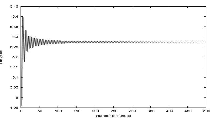
4.95 5 5.05 5.1 5.15 5.2 5.25 5.3 5.35 5.4 5.45
0 50 100 150 200 250 300 350 400 450 500
Put Value
Number of Periods
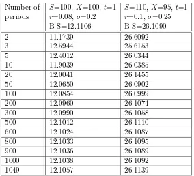
[image:36.595.86.528.437.685.2]Number of S=100,X=100,t=1 S=110,X=95,t=1 periods r=0.08,σ=0.2 r=0.1,σ=0.25
B-S=12.1106 B-S=26.1090
2 11.1739 26.6092
3 12.5944 25.6153
5 12.4012 26.0344
10 11.9039 26.0385
20 12.0041 26.1455
50 12.0650 26.0902
100 12.0854 26.0999
200 12.0960 26.1074
300 12.0990 26.1058
500 12.1012 26.1110
600 12.1024 26.1087
800 12.1033 26.1095
900 12.1036 26.1089
1000 12.1038 26.1092
[image:37.595.165.449.274.532.2]1049 12.1057 26.1139
Appendix A
BOP Model’s Convergence for a
European Call Option (Python
Codes)
from __future__ import division
from math import * import Gnuplot
from scipy import *
from scipy.linalg import *
vol=0.2 # Volatility
t=1 # Maturity
S=100 # Current price
X=100 # Strike price
r=0.08 # Risk-free interest rate
noperiod=1000 # Number of periods
data=[]
for n in range(2,noperiod): delta=t/n
u=exp(vol*sqrt(delta)) # Proportion of upward movement
d=exp(-vol*sqrt(delta)) # Proportion of downward movement
p=(exp(r*delta)-d)/(u-d) # Risk neutral probability
a0=log(X/(S*(d**n))) a1=log(u/d)
a=ceil(a0/a1)
b=(1-p)**n
for i in range(1,a+1):
b=(b*p*(n-i+1))/((1-p)*i)
D=S*(u**a)*(d**(n-a)) c=b*(D-X)*(1/R)
for j in range(a+1,n+1):
b=(b*p*(n-j+1))/((1-p)*j) D=D*(u/d)
c+=(b*(D-X))/R
data+=[[n,c]]
gp = Gnuplot.Gnuplot(persist=1)
gp(’set terminal postscript eps’) gp(’set output "BOP1.eps2"’)
gp(’set ylabel "Call Value"’)
gp(’set xlabel "Number of Periods"’)
plot10= Gnuplot.PlotItems.Data(data, with="line", title=None)
gp.plot(plot10)
gp(’set output’)
Appendix B
BOP Model’s Convergence for a
European Put Option (Python Codes)
from __future__ import division from math import *
import Gnuplot
from scipy import *
from scipy.linalg import *
vol=0.2 # Volatility
t=1 # Maturity
S=100 # Current price
X=100 # Strike price
r=0.08 # Risk-free interest rate
noperiod=1000 # Number of periods
data=[]
for n in range(2,noperiod):
delta=t/n
u=exp(vol*sqrt(delta)) # Proportion of upward movement
d=exp(-vol*sqrt(delta)) # Proportion of downward movement
p=(exp(r*delta)-d)/(u-d) # Risk neutral probability
a0=log(X/(S*(d**n)))
a1=log(u/d)
a=ceil(a0/a1) R=exp(r*t)
b=(1-p)**n
c=b*(X-D)*(1/R) for j in range(1,a):
b=(b*p*(n-j+1))/((1-p)*j)
D=D*(u/d) c+=(b*(X-D))/R
data+=[[n,c]]
gp = Gnuplot.Gnuplot(persist=1) gp(’set terminal postscript eps’)
gp(’set output "BOP2.eps2"’)
gp(’set ylabel "Put Value"’)
gp(’set xlabel "Number of Periods"’)
plot10= Gnuplot.PlotItems.Data(data, with="line", title=None) gp.plot(plot10)
gp(’set output’)
Appendix C
BOP Model’s Convergence for an
American Call Option (Python
Codes)
from __future__ import division
from math import * import Gnuplot
from scipy import *
from scipy.linalg import *
vol=0.2 # Volatility
t=1 # Maturity
S=100 # Current price
X=100 # Strike price
r=0.08 # Risk-free interest rate
noperiod=500 # Number of periods
def pay1(x0,y0): # call value
a=x0-y0 if a<=0:
b=0
else: b=a
return b data1=[]
for n in range(2,noperiod):
delta=t/n
u=exp(vol*sqrt(delta)) # Proportion of upward movement
d=exp(-vol*sqrt(delta)) # Proportion of downward movement
p=(exp(r*delta)-d)/(u-d) # Risk neutral probability
R1=exp(r*delta)
data=[]
a0=log(X/(S*(d**n))) a1=log(u/d)
a2=a0/a1
a=int(ceil(a0/a1)) for i in range(0,n+1):
data+=[0]
for i in range(0,n+1):
y=S*(u**(n-i))*(d**i)
data[i]=pay1(y,X) for i in range(n-1,-1,-1):
s=i
for j in range(0,s+1):
c=(p*data[j]+(1-p)*data[j+1])/R1
y1=(S*(u**(i-j))*(d**j))-X
data[j]=max(c,y1) data1+=[[n,data[0]]]
gp = Gnuplot.Gnuplot(persist=1)
gp(’set ylabel "Call Value"’)
gp(’set xlabel "Number of Periods"’)
plot10= Gnuplot.PlotItems.Data(data1, with="line", title=None)
Appendix D
BOP Model’s Convergence for an
American Put Option (Python Codes)
from __future__ import division from math import *
import Gnuplot
from scipy import *
from scipy.linalg import *
vol=0.2 # Volatility
t=1 # Maturity
S=100 # Current price
X=100 # Strike price
r=0.08 # Risk-free interest rate
noperiod=500 # Number of periods
def pay2(x0,y0): # Put value
a=y0-x0
if a<=0: b=0
else:
b=a return b
data1=[]
for n in range(2,noperiod): data=[]
delta=t/n
d=exp(-vol*sqrt(delta)) # Proportion of downward movement
p=(exp(r*delta)-d)/(u-d) # Risk neutral probability
R1=exp(r*delta)
data=[]
a0=log(X/(S*(d**n)))
a1=log(u/d)
a2=a0/a1
a=int(ceil(a0/a1))
for i in range(0,n+1):
data+=[0]
for i in range(0,n+1):
y=S*(u**(n-i))*(d**i) data[i]=pay2(y,X)
for i in range(n-1,-1,-1):
s=i
for j in range(0,s+1):
c=(p*data[j]+(1-p)*data[j+1])/R1
y1=X-(S*(u**(i-j))*(d**j)) data[j]=max(c,y1)
data1+=[[n,data[0]]]
gp = Gnuplot.Gnuplot(persist=1) gp(’set ylabel "Put Value"’)
gp(’set xlabel "Number of Periods"’)
Bibliography
[1] Boyle P., “Option Valuation Using a Three-Jump Process”, International Options Journal, 3, 7-12, 1986.
[2] Black F. and Scholes M., “The Pricing of Options and Corporate Liabilities”, The Journal of Political Economy, 81, 637-654, 1973.
[3] Chance D. M., “A Chronology of Derivatives”, Derivatives Quarterly, 2, 53-60, Winter, 1995.
[4] Chance D. M., Essays in Derivatives, Wiley & Sons, New Jersey, 1998
[5] Cox, J. C., Ross S. and Rubinstein M., “Option Pricing: A simplified Approach”,The Journal of Financial Economics, 7, 229-263, 1979.
[6] Kopp E., Financial Mathematics, AIMS Lecture Notes, 2004.
[7] Galitz L. C., Financial Engineering: Tools and Techniques to Manage Financial Risk, Burr Ridge, II: Irvin, 1995.
[8] Greenspan A., “Financial Derivatives”, Remarks by Chairman of Federal Reserved Bank to Futures Industry Association, Florida, March 19, 1999.
[9] Grimmett G. R. and Stirzaker D. R., Probability and Random Processes, Oxford University Press, Oxford, 2003.
[10] Hsia, C-C., “On the Binomial Option Pricing”, The Journal of Financial Research, 6, 41-46, 1983.
[11] Hull C. J.,Options, Futures and other Derivatives, Pearson Education Inc., New Jersey, 2003.
[12] Jarrow R. A. and Rudd A. R., Option Pricing, Irwin Inc., Illinois, 1983.
[14] Lyuu Y., Financial Engineering and Computation: Principles, Mathematics, and Algorithms, Cambridge University Press, Cambridge, 2002.
[15] Mackay C., Extraordinary Popular Delusions and the Madness of Crowds, Harmony Books, 1980.
[16] Marek C. and Tomasz Z.,Mathematics for Finance: An Introduction to Financial Engineering, Springer-Verlag, London, 2003.
[17] McMillan L. G., Options as a Strategic Investment, Fourth Edition, New York Institute of Finance, New York, 2002.