Correction of errors in scale values for magnetic elements for Helsinki

www.ann-geophys.net/32/633/2014/ doi:10.5194/angeo-32-633-2014

© Author(s) 2014. CC Attribution 3.0 License.

Correction of errors in scale values for magnetic elements

for Helsinki

L. Svalgaard

Stanford University, Cypress Hall C3, 466 Via Ortega, Stanford, CA 94305, USA

Correspondence to: L. Svalgaard ([email protected])

Received: 2 November 2013 – Revised: 2 April 2014 – Accepted: 28 April 2014 – Published: 5 June 2014

Abstract. Using several lines of evidence we show that the scale values of the geomagnetic variometers operating in Helsinki in the 19th century were not constant throughout the years of operation 1844–1897. Specifically, the adopted scale value of the horizontal force variometer appears to be too low by ∼30 % during the years 1866–1874.5 and the adopted scale value of the declination variometer appears to be too low by a factor of ∼2 during the interval 1885.8–1887.5. Reconstructing the heliospheric magnetic field strength from geomagnetic data has reached a stage where a reliable re-construction is possible using even just a single geomagnetic data set of hourly or daily values. Before such reconstruc-tions can be accepted as reliable, the underlying data must be calibrated correctly. It is thus mandatory that the Helsinki data be corrected. Such correction has been satisfactorily car-ried out and the HMF strength is now well constrained back to 1845.

Keywords. Geomagnetism and paleomagnetism (time vari-ations, diurnal to secular) – interplanetary physics (interplan-etary magnetic fields; instruments and techniques)

1 Introduction and rationale

After more than a decade of vigorous research (e.g., Lock-wood et al., 1999; Svalgaard et al., 2003; Svalgaard and Cliver, 2005, 2010; Lockwood and Owens, 2011) the mag-nitude of the heliospheric magnetic field (HMF) near Earth is well constrained from 1883 (probably even from 1872) to the present during which period sufficient and accurate ge-omagnetic data is available for calculation of the IDV index (Svalgaard and Cliver, 2005, 2010) that serves as a proxy for the HMF strength,B. There is still a healthy debate about the reconstruction before 1883 when geomagnetic data becomes

sparse and subject to errors, especially in the more difficult to measure horizontal force.

Although the IDV-index is calculated from the unsigned difference between the horizontal force at consecutive local midnight hours, it was already pointed out by Svalgaard and Cliver (2003, 2005) and Svalgaard and Cliver (2010, Fig. 6) that the IDV index can be computed for any hour and for any geomagnetic element. Conforming with that stipulation, Lockwood and colleagues (e.g., Lockwood et al., 2013a, b; Lockwood, 2013) have suggested to reduce the influence of noise in the early 19th century geomagnetic data by com-puting the average of the 24 individual time series of IDV calculated for each of the 24 h of the day, dubbed IDV(1d). Although this procedure introduces unwanted variance be-cause of the day-to-day variability of the (semiregular) diur-nal variation of the geomagnetic field, the “IDV signature” is robust enough such as to reduce this extra variance to a second-order effect.

Nevanlinna and colleagues (Nevanlinna et al., 1992; Nevanlinna, 2004) have compiled archived geomagnetic ob-servations from the Helsinki (IAGA – International Associ-ation of Geomagnetism and Aeronomy – designAssoci-ation HLS) magnetic observatory comprising over 2 million observations ofHandDcomponents measured during the interval 1844– 1912 with time resolution of 10 min to 1 h. Because of dis-turbances from nearby electric tram lines and general cur-tailment of the observational program, reliable and complete daily records of hourly values are only available up through 1897. Lockwood et al. (2013a, b) used this HLS data set to calculate IDV(1d).

Bartels (1925, 1932) defined the umeasure as the average (over from 1 to 12 months) unsigned difference between the daily means of the horizontal force, formally equivalent to the proposed IDV(1d) index and used by Svalgaard and Cliver (2005) in the derivation of their IDV index. Before 1872 there were no readily available daily mean data for any magnetic observatory, so Bartels – “more for illustration than for actual use” – turned to use the “summed ranges” (desig-nateds) supplied by Moos (1910) as the main contributor to a proxy for theumeasure.

Bartels’ interpretation of Moos’ procedure and data (Moos, 1910, Table 261) was “s is derived from the mean diurnal variation of H at Bombay for each single month, expressed in departures from the average, and is the sum of these departures, summed without regard to sign”. Using monthly means attenuates the irregular strong disturbances associated with the IDV signature and gives undue weight to the regular daily variation, thus downplaying the role of true “disturbances”. Moos was aware of this and on his ef-fort of making a list of days classified as quiet or disturbed (ibid. page 421) remarked that “[for] a list of the kind [. . . ] involving a large personal equation, some additional data are clearly essential in order to make the classification more mathematically definite. The daily range, or preferably the summed ranges, figures of the diurnal inequality of each day1would probably serve as the most appropriate data for this purpose; but as this is not possible on account of the heavy labour involved in their derivation”; so he resorted to the monthly means eventually used by Bartels. Here we shall build on that intuition (based on Moos’ extensive knowledge of the phenomenon) as we are no longer limited by com-putational power, provided data in digital tabular format is available. To make things explicit, Fig. 1 illustrates our in-terpretation of Moos’ prescription, emphasizing that byswe shall henceforth in this paper meansderived from daily de-partures.

2.1 Calculating IDV from summed ranges

We begin by calculating s for both the declination, s(D), and for the horizontal force, s(H ), for the German station Potsdam (POT, 1890–1907) and its replacement stations Sed-din (SED, 1908–1931) and Niemegk (NGK, 1932–2012).

1_{Italics added.}

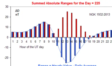
Figure 1. Average diurnal variation of declination (expressed in

force units, nT) at Niemegk. On any given day, the variation con-sists of a pattern as shown here (although varying a bit from day to day) with superposed “noise” from geomagnetic activity, thus in-creasing the variance; this increase is what we are interested in. The signed deviations (blue bars determined every hour – either from an instantaneous value on the hour or from the hourly mean) from the daily mean are converted to unsigned departures (red bars), which are then summed over the day giving (as Moos expressed it) the summed ranges for each day, denoted bys.

Geomagnetic conditions were essentially the same at all three stations, because they were carefully placed with that in mind, so we can treat the data as homogeneous from a single station (Fig. 2).

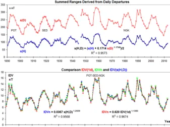
By inspection it is clear thats(D) and s(H ) are highly correlated, in facts(H )=0.1714s(D)1.1738(the coefficient of determinationR2=0.9573 is calculated from the linear fit of the logarithms); see also Fig. A1 in the Appendix. We can then form the averages(H, D)of observeds(H )ands(H ) calculated froms(D)as shown by the black line in the upper panel of Fig. 2. We can calculate the IDV index for this par-ticular station chain in the usual way using unsigned differ-ences between the hour following local solar midnight, call it IDVn. The series of IDVn ands(H, D)are also highly corre-lated: IDVn = 0.0367s(H, D)1.2029 (R2=0.9568); Fig. A2 in the Appendix. It is rare to find correlations that significant. The conclusion is that given eithers(D) or s(H ) or both, we can calculate a very close approximation (blue curve) to the usual IDVn (green curve) as shown in the lower panel of Fig. 2. This is particularly important for early stations where His often very noisy, whileDis well-observed (or at times even the only component observed).

Figure 2. (Upper panel) Summed ranges derived from daily departures for declinations(D)(red curve) and horizontal forces(H )(blue curve) for the combined POT-SED-NGK series. Each station’s yearly value is marked with a different symbol (POT diamond, SED square, NGK circle). The break in 1945 was caused by interruptions stemming from the Battle for Berlin during the final phase of WWII. The composites(H, D)is added overs(H )as a black line. It is difficult to distinguish between the blue and the black lines. It is rare in this business to find such close agreement.

(Lower panel) IDVn (from midnight values) for POT-SED-NGK (green line) compared to IDV computed froms(H, D)(blue dashed line). Because the two curves are so close to at times be indistinguishable, each yearly value is also marked with a symbol: green circle for IDVn and blue plus sign for IDV (s(H, D)). Finally, the red curve and red triangles show IDV(1d) scaled to IDVn as indicated. We need that scaling because IDV(1d) is about 11 % higher than IDVn due to the day-to-day variability of the regular daily variation.

p. 13) that “theuindex . . . certainly suffers from intrinsic de-fects . . . . One might suspect a contamination by the regular variation, since its day-to-day variability should contribute to the interdiurnal variability. However, we tried to evaluate the importance of this contamination and were astonished at its relative smallness.” So, we have essentially three differ-ent ways of estimating IDV. This also holds for other long-term homogeneous station sets, e.g., PSM(Parc Saint-Maur)-VLJ(Val Joyeux)-CLF(Chambon-la-Forêt). As long as we limit ourselves to stations far enough (>10◦) from the auro-ral zone these three different methods yield comparable and highly correlated values.

3 Scale values for Helsinki data

The original archived data for Helsinki Observatory (situated at 60◦10.40N, 24◦56.90E) was given in “scale units”, which must be converted to force units (nT, called gammas in older literature) or angles (typically tenths of arc minutes). The scale units must be converted into physical units. The usual scheme calculates the physical values from the scale units like this: physical value = base value + scale value·(scale

units + instrument corrections). Often the base value and the instrument corrections are not known and the magnetome-ter can be characmagnetome-terized only as a “variomemagnetome-ter”. The scale value must be known, either from instrument characteristics or from comparison with other instruments or other data, for the data to be of use.

Figure 3. Yearly average summed ranges forH (pink triangles) and forD(green diamonds) scaled to match the scale ofH using the equations in green for HLS (left) and ESK (right). The equations are slightly different because the inhomogeneous “raw” values are plotted, i.e., not normalized to a common “bridge”. The values ofs(H )for the interval 1866–1874.5 (orange symbols) do not match the rest of the

s(H )to scaleds(D). IDV(1d) calculated from H for ESK (purple symbols; scale on right) is a good fit tos(H )ands(D). A few “spikes” have been suppressed by capping daily IDV(1d) at 150 nT. IDV(1d) calculated fromH for HLS (scale at right; same scale as for ESK as no normalization between HLS and ESK is performed – this is raw data – for this inhomogeneous data set) is also a good fit tos(H )ands(D), except for the interval 1866–1874.5.

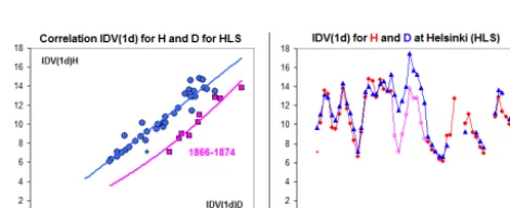
3.1 Calculating IDV(1d) fromsat ESK and HLS In Lockwood et al. (2013a, b) the IDV(1d) series for HLS and ESK (Eskdalemuir) are spliced together using POT as a “bridge”. In spite of the bridge being at considerably lower corrected geomagnetic latitude (by 6◦_{), it is posited that the}

result is a homogeneous data set. If so, results from ESK should be applicable to HLS as well. In Fig. 3 we show in the right-hand part the very similar variations since 1911 of the summed rangess(H )and ofs(D)(scaled tos(H )) and of IDV(1d) for ESK. This is as expected from the results demonstrated in Sect. 2. For HLS, shown in the left-hand part of the figure,s(H )and (scaled)s(D)also agree closely, ex-cept for the interval 1866–1874.5 (orange data points). The simplest, and in our view inescapable, conclusion to draw from this discrepancy is that the adopted scale value of the H variometer was too small, by some 30 %, during the in-terval 1866–1874.5. Figure A3 in the Appendix compares IDV(1d) for HLS calculated from the summed ranges, fur-ther visualizing the obvious discrepancy. IDV(1d) for HLS, calculated for years outside of the interval 1866–1874.5 is plotted in Fig. 3 as well, for comparison. The agreement with s(H )ands(D)is again good.

4 IHV also shows the scale value discrepancies

Svalgaard and colleagues (Svalgaard et al., 2003, 2004; Sval-gaard and Cliver, 2007) introduced the interhourly variability index, IHV, as a proxy for auroral zone activity (as measured at midlatitudes). Although HLS is too close to the auroral zone for IHV calculated from HLS data to retain its simple physical meaning (a proxy for solar wind BV2 and for the NOAA/POES hemispheric power; Emery et al., 2008), the IHV values do depend directly on the scale value used for the variometers. As for IDV, IHV can be computed for any geo-magnetic element. If the scale values forH and forDwere

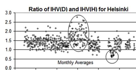
Figure 4. The ratio between monthly values of IHV calculated

us-ing the declination, IHV (D), and of IHV calculated using the hori-zontal force, IHV (H) for Helsinki. The ovals show the effect of the scale value forHbeing too low in the interval 1866–1874.5 and of the scale value forDbeing too low in the interval 1885.8–1887.5.

both correct, the ratio between IHV (D) and IHV (H) would be constant (apart from a random noise component). Figure 4 shows the ratio between IHV (D) and IHV (H) for HLS. As predicted from the analysis in Sect. 3 the ratio shows the ex-pected behavior (in large oval) for the interval 1866–1874.5. The smaller oval shows that there is also a problem with the scale value of theDvariometer in the interval 1886–1887.5, being too low by about a factor of 2. This is explored further in the Appendix (Fig. A5).

5 The daily variation

Figure 5. Yearly average ranges for declinationD(in 0.1 arc minute units), blue curve, and for horizontal force (in nT units), pink curve. Because of the strong seasonal variation only years with no more than a third of the data missing are plotted. The green curve (with “+” symbols) shows the number of active regions (sunspot groups) on the disk scaled to match the pink curves (H). As expected the match is excellent, except for the interval 1866–1874, where theH range would have to be multiplied by 1.32 for a match, purple open circles.

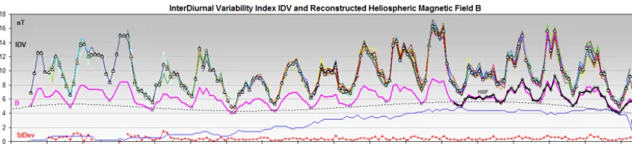
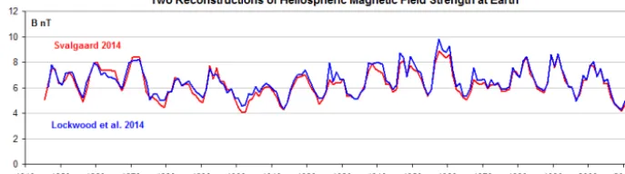
Figure 6. Reconstruction of annual means of 169 years of near-Earth heliospheric magnetic field strengthB(pink line in middle of graph) for the interval 1845–2013 compared with in situ spacecraft measurements (black line marked HMF) plotted using different colors for each station, from Svalgaard and Cliver (2014). Open triangles (or circles) show the median (or mean) of all stations in each year. The red line at the bottom of the graph shows the standard deviation of the values of IDV in each year. The blue line markedNshows the number of stations for each year.

(slowly varying) secular values and of random (unknown) changes in the baseline. The average, over an interval – such as a month or a year – of the differences as a function of time within the day is the average diurnal variation (what used to be called the daily “inequality”). It is well-known that that average range, i.e., the difference between the max-imum and minmax-imum values of the average diurnal variation, is extremely well correlated with appropriate solar activity indices (e.g., F10.7 microwave flux, sunspot number, or the group number (number of active regions on the solar disk)), as was discovered by Wolf (1852)2and subsequently exten-sively verified by many workers (e.g., Bartels, 1946), con-sidered to be the best of all solar–terrestrial correlations; a fact used by Nevanlinna et al. (1992), who note “(t)he scale value for theD variometer seems to be reliable (for 1844– 1853) because the diurnal variation at the Helsinki, Nur-mijärvi and St. Petersburg observatories show very similar

2_{“Wer hätte noch vor wenigen Jahren an die Möglichkeit}

gedacht, aus den Sonnenfleckenbeobachtungen ein terrestrisches Phänomen zu berechnen?” (Who would have thought, just a few years ago, of the possibility of computing a terrestrial phenomenon from observations of sunspots?)

behavior being the same within 1’ under corresponding so-lar activity conditions”. Figure 5 shows the yearly average ranges forDandHat Helsinki.

The group numbers used in Fig. 5 are derived from the recent re-evaluation of solar activity (Svalgaard, 2013). Us-ing the official SIDC (Solar Influences Data Center) sunspot number does not change the result for the interval of inter-est (Appendix, Figs. A4, A5). It seems that the scale value adopted forH during the interval 1866–1874 must actually be different from that used for the rest of theHdata, specifi-cally 1.32 times lower than the constant value used by Nevan-linna (2004) in constructing the Helsinki series. The range of the declination during that interval matches that ofH when H is rescaled upwards by the factor 1.32. The ranges ofD andHgenerally vary together (with solar activity) due to the same current system, so the discrepancy indicates a problem with the adopted scale value ofH. Figure A4 in the Appendix documents the problem for the H component for the year 1869, while Fig. A5 in the Appendix documents the problem for the declination for the year 1886.

et al. (2014a) (blue curve). The coefficient of determination isR =0.93.

stations, not using the solar activity connection. In Fig. A6 of the Appendix, we show a comparison with Greenwich (GRW, brown), Prague (PRA, blue), and Colaba (CLA and replacement station Alibag ABG, green). Because not all sta-tions observed hourly values all the time, the ranges have been matched to Helsinki (HLS, pink) outside the interval 1866–1874. During that interval, the range for HLS (red tri-angles) is seriously too low.

6 Reconstructed HMF

Figure 6 shows a reconstruction of annual means of 169 years of near-Earth heliospheric magnetic field strength B (pink line in middle of graph) for the interval 1845–2013 compared with in situ spacecraft measurements (black line marked HMF). The reconstruction is based on a re-evaluation of the IDV index using the normalized average of the three determinations discussed in Sects. 2 and 3, from Svalgaard and Cliver (2014), plotted using different colors for each sta-tion. For the interval 1863–1871 leading up to the strong so-lar cycle 11, only HLS contributes (awaiting digitization of other stations), underscoring the importance of getting HLS right.

A consequence of the undue weight given to the regular diurnal variation that we referred to in Sect. 2 when using the summed ranges based on monthly averages that Bartels used to extend the u measure before 1872 is that our ear-lier reconstruction based on the u measure (Svalgaard and Cliver, 2010) for years with large coronal holes and ensu-ing large HMF durensu-ing the declinensu-ing phase of the solar cycles was too low for years during the declining phase. Going to the summed daily ranges,s(H, D), remedies that defect, es-pecially when the erroneous scale values are corrected. It is instructive to compare the reconstruction for solar cycles 10 and 11 (1857–1878) with those of cycles 18 and 19 (1945– 1964), as regard to both the “shape” of the solar cycle curves and to the similar general level of activity.

After the present paper was submitted, Lockwood et al. (2014a; 2014b) and Lockwood and Owens (2014), now aware of our finding, have accepted our analysis and cor-rected their reconstruction accordingly. Figure 7 shows that their revised values (Lockwood et al., 2014a) are largely correct (compared with our multistation reconstruction), and that reconstruction of the HMF strength is now satisfactory constrained back to 1845. A significant insight that follows from the concordant reconstructions is that there hardly was any “modern grand maximum” as the values of the HMF in the 20th century are on par with the values in the mid-19th century.

7 Conclusion and recommendations

Appendix A

In this section we collect various Figures providing supple-mentary support for the analysis in the paper.

Figure A1. The averages(H )for each year is plotted against the averages(D)for that year. The data can be fitted to a power law as shown, which “explains” 96 % of the correlation. We use power laws because most regression plots show somewhat curved point clouds (“rivers” is probably a more descriptive term).

Figure A2. Correlation between yearly values of IDVn (midnight) and the average summed ranges for the day forH andD,s(H, D), for the POT-SED-NGK composite series for the interval 1890–2012. The dashed line is the linear relation extrapolated to vanishing IDVn.

range ofDis about the same for the 3 years shown. The timing from 1882 on has been adjusted to 1 h later (also in the following figure) because of a change from Göttingen time to local Helsinki time, which is not reflected correctly in the published data.

Figure A5. Diurnal variation ofH (left) and ofD(right) at Helsinki for 3 years with a SIDC sunspot number of∼25. It is very hard to escape the conclusion that the range ofDfor the year 1886 is too small compared to the other years with a similar sunspot number as the range ofH is about the same for the 3 years shown. Detailed analysis shows that the problem exists from October 1885 to May 1887. In August 2003 we emailed Nevanlinna alerting him to this problem, but, unfortunately, no corrective action resulted from this. It is now clear that scale-value problems exist for both theH component and for the declination and that corrective action is mandatory before use of the Helsinki data.

Figure A6. The diurnal range (in nT) of the horizontal force for Prague (PRA) blue, Colaba (CLA)+Alibag (ABG) green, Greenwich (GRW)

Acknowledgements. We acknowledge the impetus from

participat-ing in work of the ISSI International Team 233 and from servparticipat-ing as reviewers of Lockwood et al. (2013a, b). The Helsinki data was downloaded from http://wdc.kugi.kyoto-u.ac.jp/ and cleaned for the usual types of errors found in such data sets, like data for 31 Novem-ber, time being off by 1 h from 1882 on, and base values for decli-nation being expressed in tens of minutes rather than the (correct) degrees. L. Svalgaard appreciates the continuing support from Stan-ford University.

Topical Editor C. Owen thanks T. L. Hansen and two anony-mous referees for their help in evaluating this paper.

References

Bartels, J.: Archiv des Erdmagnetismus, Heft 5, Abh. Met. Inst., 8, Berlin, 1925.

Bartels, J.: Terrestrial-magnetic activity and its relations to solar phenomena, Terr. Magn. Atmos. Elec., 37, 1–52, 1932. Bartels, J.: Geomagnetic data on variations of solar radiation, 1,

Wave-radiation, Terr. Magn. Atmos. Elec., 51, 181–242, 1946. Emery, B. A., Coumans, V., Evans, D. S., Germany, G. A.,

Greer, M. S., Holeman, E., Kadinsky-Cade, K., Rich, F. J., and Xu, W.: Seasonal, Kp, solar wind, and solar flux varia-tions in long-term single-pass satellite estimates of electron and ion auroral hemispheric power, J. Geophys. Res., 113, A06311, doi:10.1029/2007JA012866, 2008.

Lockwood, M.: Reconstruction and Prediction of Variations in the Open Solar Magnetic Flux and Interplanetary Conditions, Living Rev. Solar Phys. 10, 4, doi:10.12942/lrsp-2013-4, 2013. Lockwood, M. and Owens, M. J.: Centennial changes in the

heliospheric magnetic field and open solar flux: The con-sensus view from geomagnetic data and cosmogenic iso-topes and its implications, J. Geophys. Res., 116, A04109, doi:10.1029/2010JA016220, 2011.

Lockwood, M. and Owens, M. J.: Implications of the Recent Low Solar Minimum for the Solar Wind During the Maun-der Minimum, Astrophys. J. Lett., 781, 1, doi:10.1088/2041-8205/781/1/L7, 2014.

Lockwood, M., Stamper, R., and Wild, M. N.: A doubling of the Sun’s coronal magnetic field during the past 100 years, Nature, 399, 437–439, doi:10.1038/20867, 1999.

Lockwood, M., Barnard, L., Nevanlinna, H., Owens, M. J., Har-rison, R. G., Rouillard, A. P., and Davis, C. J.: Reconstruction of geomagnetic activity and near-Earth interplanetary conditions over the past 167 yr – Part 1: A new geomagnetic data compos-ite, Ann. Geophys., 31, 1957–1977, doi:10.5194/angeo-31-1957-2013, 2013a.

Lockwood, M., Barnard, L., Nevanlinna, H., Owens, M. J., Har-rison, R. G., Rouillard, A. P., and Davis, C. J.: Reconstruc-tion of geomagnetic activity and near-Earth interplanetary con-ditions over the past 167 yr – Part 2: A new reconstruction of the interplanetary magnetic field, Ann. Geophys., 31, 1979–1992, doi:10.5194/angeo-31-1979-2013, 2013b.

Lockwood, M., Nevanlinna, H., Vokhmyanin, M., Ponyavin, D., Sokolov, S., Barnard, L., Owens, M. J., Harrison, R. G., Rouil-lard, A. P., and Scott, C. J.: Reconstruction of geomagnetic ac-tivity and near-Earth interplanetary conditions over the past 167 yr – Part 3: Improved representation of solar cycle 11, Ann. Geo-phys., 32, 367–381, doi:10.5194/angeo-32-367-2014, 2014a.

Lockwood, M., Nevanlinna, H., Barnard, L., Owens, M. J., Har-rison, R. G., Rouillard, A. P., and Scott, C. J.: Reconstruc-tion of geomagnetic activity and near-Earth interplanetary con-ditions over the past 167 yr – Part 4: Near-Earth solar wind speed, IMF, and open solar flux, Ann. Geophys., 32, 383–399, doi:10.5194/angeo-32-383-2014, 2014b.

Mayaud, P. N.: Derivation, Meaning, and Use of Geomagnetic In-dices, Geophys. Monogr. Ser., Vol. 22, 154 pp., ISBN 0-87590-022-4, American Geophysical Union, Washington D.C., 1980. Morozova, A. L., Ribeiro, P., and Pais, M. A.: Correction of

ar-tificial jumps in the historical geomagnetic measurements of Coimbra Observatory, Portugal, Ann. Geophys., 32, 19–40, doi:10.5194/angeo-32-19-2014, 2014.

Moos, N. A. F.: Colaba Magnetic Data, 1846 to 1905, 2, The Phe-nomenon and its Discussion, 782 pp., Central Govt. Press, Bom-bay, 1910.

Nervander, J. J.: Observations faites à l’observatoire Magnétique et Météorologique de Helsingfors 1844–1848, Vol. I–IV, Helsing-fors, 1850.

Nevanlinna, H.: Results of the Helsinki magnetic observatory 1844– 1912, Ann. Geophys., 22, 1691–1704, doi:10.5194/angeo-22-1691-2004, 2004.

Nevanlinna, H., Ketola, A., and Kangas, T.: Magnetic Results from Helsinki Magnetic-Meteorological Observatory, Finn. Met. Inst., Geophys. Publ., 27, 155 pp., 1992.

Svalgaard, L.: Building a Sunspot Group Number Backbone Series, available at: http://www.leif.org/research/SSN/Svalgaard11.pdf (last access: 3 June 2014), 2013.

Svalgaard, L. and Cliver, E. W.: New Geomagnetic Index (IDV) Measuring Magnitude of Interplanetary Magnetic Field, AGU Fall SH21B-0108, available at: http://www.leif.org/research/ AGUFall2003SH21B-0108.pdf (last access: 3 June 2014), 2003. Svalgaard, L. and Cliver, E. W.: The IDV index: Its derivation and use in inferring long-term variations of the interplane-tary magnetic field strength, J. Geophys. Res., 110, A12103, doi:10.1029/2005JA011203, 2005.

Svalgaard, L. and Cliver, E. W.: Interhourly variability index of ge-omagnetic activity and its use in deriving the long-term vari-ation of solar wind speed, J. Geophys. Res., 112, A10111, doi:10.1029/2007JA012437, 2007.

Svalgaard, L. and Cliver, E. W.: Heliospheric mag-netic field 1835–2009, J. Geophys. Res., 115, A09111, doi:10.1029/2009JA015069, 2010.

Svalgaard, L. and Cliver, E. W.: Update: Heliospheric magnetic field 1835–2013, J. Geophys. Res., in preparation, 2014.

Svalgaard, L., Cliver, E. W., and Le Sager, P.: Determination of in-terplanetary magnetic field strength, solar wind speed, and EUV irradiance, 1890–2003, in Proceedings of ISCS 2003 Sympo-sium: Solar Variability as an Input to the Earth’s Environment, Eur. Space Agency Spec. Publ., ESA SP-535, 15, 2003. Svalgaard, L., Cliver, E. W., and Le Sager, P.: IHV: A new

long-term geomagnetic index, Adv. Space. Res., 34, 1112–1120, doi:10.1016/j.asr.2007.06.066, 2004.