Randomization and American Puts

Randomization and the American Put

Peter Carr

Morgan Stanley

1585 Broadway, 6th oor

New York, NY 14853

(212) 761-7340

E-mail:[email protected]

September 22, 1997

I thank the participants of presentations at the 1996 AFA conference, the 1996 Columbia University conference on

Randomization and the American Put

Abstract

Closed-form solutions for the value of European-style options have been known since the seminal papers of Black-Scholes (1973) and Merton (1973). Since American calls on non-dividend paying stocks are not rationally exercised early, they can be valued in closed form. Unfortunately, the vast majority of listed options are American-style and subject to early exercise. Despite a profusion of research on the subject, no completely satisfactory analytic solution for the value of such options has been found.

The principal diculty in obtaining an analytic solution arises from the absence of a simple expression for the optimal exercise boundary. An exercise boundary is a time path of critical stock prices at which early exercise occurs. The optimal exercise boundary of an American option is not known ex ante, and must be determined as part of the solution to the valuation problem. Furthermore, it is dicult to analytically approximate American option values using boundary approximations which are consistent with the known short and long time behavior of the exercise boundary.

The purpose of this paper is to develop a new approach for determining American option values and exercise boundaries based on a technique called randomization. In general, randomization describes a three step procedure which can be used to solve a host of problems. The rst step is to randomize a parameter by assuming a plausible distribution for it. The second step is to somehow calculate the expected value of the dependent variable in this random parameter setting. This is the dicult step since one does not know the dependent variable in the xed parameter setting. The nal step is to let the variance of the distribution governing the parameter approach zero, holding the mean of the distribution constant at the xed parameter value.

determined by the waiting time to a pre-specied number of jumps of a standard Poisson process, which is assumed to be independent of the underlying stock price process. We note that the only role of the Poisson process is to determine maturity the stock price process used is continuous.

A random maturity contract has a value which approximates the value of its xed maturity coun-terpart. In order to distinguish between these values, we refer to the former values as randomized. Our formulas for randomized values are generally simpler than the formulas for xed maturity contracts. The simplest expression arises when the randomized American option matures at the rst jump time of a Poisson process, in which case the maturity date is exponentially distributed. This random horizon problem is equivalent to an innite horizon problem with an adjusted discount rate, as shown in a port-folio optimization setting by Merton (1971) and Cass and Yaari (1967). In the option pricing context, American options with innite horizons were valued long ago by Samuelson (1965) and McKean (1965). So it is somewhat natural1 that randomizing the maturity will lead to simpler option valuation formulas.

For American options, the simplicity of the solution arising from randomization is mainly due to the taming of the behavior of the exercise boundary. When the option matures with the rst jump, the memoryless property of the exponential distribution implies that the exercise boundary is independent of time. As calendar time elapses, the option gets no closer to its random maturity, and thus its value suers no time decay. The stationarity in value implies that the exercise boundary is also independent of time. When the underlying security has either no dividends or a constant continuous dividend ow, we can solve explicitly for the critical stock price. In contrast, if the underlying pays continuous proportional dividends, then a fairly simple algebraic equation must be solved numerically. As a result, the general formulation leads to semi-explicit valuation formulas.

Pois-son process. The maturity time is thereby Erlang distributed with a mean equal to the xed maturity date of the true American option. In this case, the exercise boundary takes the form of a staircase, with the levels being determined by optimizing within each sub-period. The resulting expression for the randomized option value is a triple sum, involving no special functions other than the natural log.

As the number of random sub-periods becomes large, the variance of the random maturity approaches zero, so that the probability density function governing maturity approaches a Dirac delta function centered at the American option's xed maturity. Thus, increasing the number of periods increases the accuracy of the solution at the expense of greater computational cost. However, when Richardson extrapolation is used, our numerical results indicate that our randomized option value converges to the true American option value in a computationally ecient manner.

The randomization approach taken in this paper is to exactly value a contract which approximates the nature of an American option. An alternative approach is to approximate the valuation operator rather than the contract. This is the approach taken when nite dierences (see eg. Brennan and Schwartz (1977)) are used to numerically solve the partial dierential equation (p.d.e.) governing the value of an American option. As is well-known, the standard nite dierence approach replaces all of the partial derivatives in a p.d.e. with nite dierences. When only the time derivative is discretized, the approach is termed the (horizontal) method of lines or Rothe's method (see Rothe (1930) and Rektorys (1982)). The application of the method of lines to free boundary problems has been promulgated in Meyer (1970), Meyer (1979) and in Meyer & van der Hoek (1994), who use it to numerically value American options. Goldenberg and Schmidt (1995) test this numerical scheme against other approaches and nd that it is highly accurate, although slightly slower2 than some other approaches. Carr and Faguet (1994) gave a

semi-explicit solution to the sequence of ordinary dierential equations which arise when the method of lines is applied to the Black Scholes p.d.e. In fact, the solution obtained via randomization in this paper is mathematically equivalent to the solution in Carr and Faguet.

American puts in the Black-Scholes model. The following section presents the randomization technique in the context of valuing an American put on a non-dividend-paying stock with an exponential maturity. The subsequent section discusses the more general case of a Erlang distributed maturity. The following section discusses the implementation of our formula and compares this implementation with extant approaches in terms of both speed and accuracy. The penultimate section extends the analysis to dividends and American calls. The nal section summarizes, while the appendix collects all the formulas needed to implement the randomization approach.

1 American Put Valuation in the Black-Scholes Model

In this section, we focus on the valuation of American puts in the Black-Scholes model. We defer the corresponding development for American calls until dividends have been introduced. The Black-Scholes model assumes that over the option's life 0

T

], the economy is described by frictionless markets, no arbitrage, a constant riskless rate

r >

0, no dividends from the underlying stock, and that the underlying spot price process f

S

t

t

2(0

T

)gis a geometric Brownian motion with a constant volatility rate

>

0.

Let

P

(

tS

T

) denote the value of an American put as a function of the current time

t

, the current stock price

S

, and the maturity date

T

. The critical stock price

S

(

t

T

)

t

2 0

T

] is dened as the largest

price

S

at which the American put value

P

(

tS

T

) equals its exercise value

K

;

S

, where

K

is the strike

price. As the maturity is shortened, the alive American put value falls, while the exercise value remains constant. A reduction in time to maturity therefore raises the critical stock price at which exercise occurs. When graphed against time, the critical stock price is a smoothly increasing function termed the exercise boundary.

For quite general stochastic processes, the American put's initial value is given by the solution to an optimal stopping problem:

P

(0

S

T

) = sup

s20T]

E

0S

f

e

;rs

K

;

S

s] +

g

(1)

In the Black-Scholes model, this optimal stopping time is the earlier of maturity and the rst passage time to the exercise boundary. Consequently, the alive American put may alternatively be valued as:

P

(0

S

T

) = sup

B(t) t20T]

E

0S

f

e

;r(B^T)

K

;

S

B

^T] +

g

S > S

(0

T

)

(2)

where

B is the rst passage time3 from

S

to an exercise boundary

B

(

t

)

t

20

T

].

McKean (1965) showed that an application of It^o's lemma to (1) implies that the alive American put value and exercise boundary jointly solve a free boundary problem, consisting of the Black-Scholes partial dierential equation (p.d.e.):

2

2

S

2

P

ss(

tS

T

)+

rSP

s(

tS

T

);

rP

(

tS

T

) =

P

T(

tS

T

)

S

2(

S

(

t

T

)

1)

t

2(0

T

)

(3)

and the following boundary conditions:

P

(

TS

T

) = (

K

;

S

) +

S

2(

S

(

T

T

)

1)

and

S

(

T

T

) =

K

lim

S"1

P

(

tS

T

) = 0

_S lim

#S(tT)

P

(

tS

T

) =

K

;

S

(

t

T

)

lim

S#S(tT)

P

s(

tS

T

) =;1

t

2(0

T

)

:

Unfortunately, there is no known exact and completely explicit solution to either the optimal stopping problem (1) or to the free boundary problem (3). The next section presents a new approach for obtaining approximate solutions to these problems.

2 Exponential Maturity Valuation

In order to obtain an approximate solution for the value of an American put and its exercise boundary, we now suppose that the maturity date is random. Let

denote the random maturity time. In this section, we assume that

is exponentially distributed with scale parameter

:

Probf

2

dt

g=

e

;t

dt:

Since the mean of

is the reciprocal of

, we set

= 1

T, so that the mean maturity of the randomized

American put, which matures at the rst jump time of a standard Poisson process with intensity

= 1

T.

We assume that the Poisson process is independent of the stock price process. Furthermore, we assume that the Poisson process is also uncorrelated with any market factor. It follows that the risk associated with the randomness of maturity can be diversied away by holding a large portfolio of random maturity options on dierent stocks. Thus, the randomized value can be calculated in a \risk-neutral" fashion.

The analog to (2) for randomized American option values is:

P

(1)(

S

) = sup

B

E

0S f

e

;r(B^)

K

;

S

B

^] +

g

S > S

1

(4)

where

S

1 is the unknown optimal exercise boundary. Note that the supremum is taken only over

time-stationary boundaries

B

rather than functions of time

B

(

t

). The memoryless property of the exponential distribution implies that the passage of time has no eect on either the randomized option value or its optimal exercise boundary. Thus, the time-dependent exercise boundary becomes at prior to the random maturity. When the Poisson process governing maturity jumps up, the randomized option value jumps down to intrinsic value (

K

;

S

)

+. Thus, one can think of the pent up time decay of the option as being

released at the jump time. This release causes the exercise boundary to jump up from

S

1 to

K

, crudely

approximating the behavior of the true exercise boundary.

The expectation in (4) can be evaluated in closed form and the result can be maximized over barriers analytically. Since the details are cumbersome, a perhaps simpler approach is to recognize the following relationship between random and xed maturity4 put values:

P

(1)(

S

) = sup

B

Z

1

0

e

;t

D

(0

S

t

B

)

dt

(5)

where

D

(0

S

T

B

) is the initial value of a down-and-out put with xed maturity

T

, out barrier

B

, and rebate

K

;

B

:

D

(0

S

t

B

) =

E

0S f

e

;r(B^T)

K

;

S

B ^T]

+

g

S > B:

One can immediately observe that the randomized American put value is simply the Laplace-Carson5

Black-Scholes p.d.e. (3), one can take the Laplace-Carson transform of both sides of this p.d.e. to obtain the following simpler ordinary dierential equation (o.d.e.):

2

2

S

2

P

(1)

ss (

S

) +

rSP

(1)

s (

S

);

rP

(1)(

S

) =

P

(1)(

S

)

;(

K

;

S

)

+]

S > S

1

(6)

subject to the following boundary conditions:

lim

S"1

P

(1)(

S

) = 0

lim

S#S 1

P

(1)(

S

) =

K

;

S

1

lim

S#S 1

P

(1)

s (

S

) =;1

:

(7)

Using standard techniques for solving o.d.e.'s, the randomized value of an American put can be decomposed as:

P

(1)

(

S

) =

8

<

:

p

(1)(

S

) +

b

(1)(

S

) if

S > S

0

K

KR

;

S

+

c

(1)(

S

) +

b

(1)(

S

) if

S

2(

S

1

S

0)

K

;

S

if

S

S

1,

(8)

where

p

(1)(

S

) is the randomized value of a European put paying (

K

;

S

)

+at the rst jump time:

p

(1)

(

S

) =

S

K

;

(

qKR

;

qK

^ )

S > K

(9)

with

1

2 ; r

2

R

1 1+rT q

2+ 2

R2T

and:

p

;

2

q

1;

p

p

^

;

+ 1

2 and ^

q

1;

p

^ (10)

b

(1)(

S

) is the present value of interest received below the critical stock price

S

1 until the rst jump time:

b

(1)

(

S

) =

S

S

1

;

qKRrT

(11)

and nally,

c

(1)(

S

) is the randomized value of a European call paying (

S

;

K

)

+at the rst jump time:

c

(1)

(

S

) =

S

K

+

(^

pK

;

pKR

)

S < K:

(12)

Kim (1990). Note that the formula (9) for the randomized value of the European put is simpler than the Black Scholes formula in that it does not use any special functions such as the normal distribution function. On the other hand, (9) holds only for out-of-the-money values (

S > K

). In contrast to the Black Scholes put formula which holds for all positive stock prices, formula (9) which values the put when

S > K

does not correctly value the put when

S < K

. The lack of smoothness in the payo function implies that Put Call Parity6 must be used to generate in-the-money values for European puts with

random maturity. The second line of our formula (8) reects this restriction. The third line of (8) sets the randomized put value to exercise value below the critical stock price

S

1. Figure 1 graphs the value

of an exponential maturity American put against the stock price. The function is twice dierentiable at the strike price, but only once dierentiable at the exercise boundary, as is the case for a true American put.

Imposing value-matching in (8) at the critical stock price

S

1 yields the following balance equation:

c

(1)(

S

1) =

pKRrT:

(13)

The left hand side is clearly the randomized value of a European call when the stock price is at the critical stock price. The right hand side represents the randomized value of a claim paying interest on the strike price at all stock prices above the current stock price level. The critical stock price is chosen so that the call value just matches the present value of the interest ow received above the boundary. Stationarity in the values involved implies that the exercise boundary remains at at this level until the jump time.

The simple expression (12) for the European call value implies that the balance equation (13) can be explicitly solved for our rst approximation to the exercise boundary,

S

1:

S

1 =

K

pRrT

^

p

;

Rp

1

+

:

(14)

For future use, note that substituting (14) into (12) implies that the randomized value of a European call is given by a formula similar to that of the randomized early exercise premium in (11):

c

(1)(

S

) =

S

S

1

+

pKRrT

A

(1)(

S

)

:

Equations (8) and (14) represent the randomized versions of the American put value and critical stock price respectively. While these rst approximations are simple and explicit, numerical implementation indicates substantial undervaluation of the put. The reason the randomized value is substantially smaller than the true value is that the owner of a random maturity put must optimize over boundaries without the benet of knowing when the option will mature.

Clearly, the valuation error can be reduced by lowering the variance of the distribution governing maturity. Unfortunately, if a random variable with an exponential distribution has mean

T

, then its variance is

T

2. The next section uses a two parameter distribution for maturity, which permits keeping

the mean maturity constant at

T

, while reducing the variance as much as desired. As the variance approaches zero, the result is a de facto inversion of the Laplace-Carson transform (8), yielding an accurate approximation of the American put value.

3 Erlang Maturity Valuation

Consider an investor who is faced with the problem of allocating his investable wealth among

n

dierent securities. If the security returns are independently and identically distributed (i.i.d.), the variance minimizing allocation is to invest an equal proportion in each security. By the same token, a simple and ecient way to reduce the variance of our option's random maturity is to split it into

n

i.i.d sub-periods. If we also assume that each of the

n

periods is exponentially distributed with parameter

, then the maturity date

is Erlang distributed:

Probf

2

dt

g=

n

(

n

;1)!

In order that the mean maturity be

T

, each subperiod must have mean4

T=n

, which implies

= 1

=

4.

By assuming that the maturity is Erlang distributed instead of exponentially distributed, the variance is reduced by a factor of 1

n to only

T

2

=n

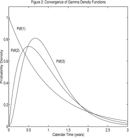
. Figure 2 shows three Erlang density functions, with each

corresponding to a maturity of mean

T

= 1 year, and with variances of 1, 1

=

2, and 1

=

3 respectively. The densities are converging to a Dirac delta function centered at

T

= 1 year.

Let

P

(n)(

S

) denote the randomized value of an American put option which can be exercised for

(

K

;

S

)

+ at any time up to and including the

n

-th jump time of a standard Poisson process (with

intensity

= 1

=

4). To value this put, we use dynamic programming. Accordingly, suppose that

n

;1

jumps have occurred and that the investor is holding a put maturing at the next jump time of the Poisson process. This valuation problem was solved in the previous section, with the solution

P

(1)(

S

) given by

(5), except that

T

must be everywhere replaced by4

T=n

.

We now back up a random time period and think of

P

(1)(

S

) as the random payo occurring at the

end of this random period, provided that no exercise has occurred beforehand. Since exercising yields a payo of (

K

;

S

)

+ as usual, the randomized value of the American put with two jumps to maturity is:

P

(2)

(

S

) =sup

B>0

E

Sf

e

;rB

K

;

B

] +

1(

B

<

2) +

e

;r

2

P

(1)

(

S

2)1(

B

2)

g

S > S

2

(15)

where

2 denotes the length of the second random period prior to maturity and

S

2 denotes the unknown

optimal exercise boundary over this period. Once again, the stationarity of the barrier

B

over the period implies that the expectation in (15) can be evaluated in closed form and the result can be maximized over barriers analytically.

As in the previous section, a perhaps simpler approach is to work with Laplace-Carson transforms. Proceeding by analogy with the previous section, let

D

(

S

T

;

tB

) denote the time

t

value of a

down-and-out put with xed maturity

T

, out barrier

B

, and which pays a rebate of

K

;

B

at the rst passage

time to

B

, if this occurs before

T

, and which pays

P

(1)(

S

the Black Scholes p.d.e.:

2

2

S

2

D

ss(

S

T

;

tB

) +

rSD

s(

S

T

;

tB

);

rD

(

S

T

;

tB

) =

D

T(

S

T

;

tB

)

S

2(

B

1)

t

2(0

T

)

(16)

subject to the terminal condition

D

(

S

0

B

) =

P

(1)(

S

) and the boundary conditions:

lim

S"1

D

(

S

T

;

tB

) = 0

lim

S#B

D

(

S

T

;

tB

) =

K

;

B

t

2(0

T

)

:

The randomized value of the American put maturing after two more jumps of the Poisson process is related to this xed maturity claim by:

P

(2)(

S

) = sup

B

Z

1

0

e

;t

D

(

S

tB

)

dt:

(17)

Taking Laplace-Carson transforms of both sides of the p.d.e. (16) implies that:

2

2

S

2

P

(2)

ss (

S

) +

rSP

(1)

s (

S

);

rP

(2)

(

S

) =

P

(2)

(

S

);

P

(1)

(

S

)]

S > S

2

(18)

subject to the following boundary conditions:

lim

S"1

P

(2)(

S

) = 0

lim

S#S 2

P

(2)(

S

) =

K

;

S

2

lim

S#S 2

P

(2)

s (

S

) =;1

:

(19)

This simpler free boundary problem can be solved analytically for both the randomized put value

P

(2)(

S

)

and the critical stock price

S

2. The graph of the American put value is similar to Figure 1, but with

slightly higher value due to the lower variance in maturity. Figure 3 shows the exercise boundary for a realization in which the rst jump happened to occur 0

:

53 years after issuance, while the put matured with the second jump 0

:

93 years after issuance. The critical stock price over the earlier of the two periods is below the critical stock price of the later period because the end of period payo is greater (i.e.,

P

(1)(

S

)

K

;

S

).

More generally, let

P

(m)(

S

) and

S

m respectively denote the randomized put value and exercise

bound-ary stair levels with

m

random periods to maturity,

m

= 0

1

:::n

, with

P

(0)(

S

)

(

K

;

S

)

+and

S

0

Then

P

(m)(

S

) and

S

m jointly solve the following sequence of free boundary problems:

2

2

S

2

P

(m)

ss (

S

) +

rSP

(m)

s (

S

);

rP

(m)(

S

) =

P

(m)(

S

) ;

P

(m;1)(

S

)]

for

S

2(

S

m

1)

(20)

subject to the boundary conditions:

lim

S"1

P

(m)(

S

) = 0

lim

S#Sm

P

(m)(

S

) =

K

;

S

m

lim

S#Sm

P

(m)

s (

S

) =;1, for

m

= 1

:::n:

(21)

Substituting

1

4 on the right side of (20) and comparing with the Black Scholes p.d.e. (3)

indicates an alternative interpretation of the approximation induced by our randomization procedure. Our randomized put value

P

(m)(

S

) is also the approximation for

P

(

T

;

m

4

S

T

) which arises when

time is discretized and the maturity derivative

P

T(

tS

T

) @P

@T(

tS

T

) in (3) is replaced with the

nite dierence P(m) (S);P

(m;1) (S)

4 =

4P (m)

(S)

4 . Note however that the spatial derivatives are not replaced

with their nite dierences, in contrast to standard nite dierence schemes or the binomial model.7 As

mentioned in the introduction the notion of discretizing one variable while leaving the other continuous is known in the numerical methods literature as semi-discretization or the method of lines.

The accuracy of our approach may be anticipated a priori by noting that as the maturity date

T

approaches innity holding the number of periods

n

xed, then

#0 and thus the problem (20) describing

the randomized put value approaches that of the perpetual put. As a result, the randomized put solution with any number of jumps remaining will converge to the correct perpetual solution. Conversely, as

n

gets arbitrarily large with

T

held xed, then the nite dierence 4P

(m) (S)

4 on the right side of (20) converges to

the maturity derivative

P

T(

tS

T

) in (3). As a result, we conjecture8 that the solution (

P

(n)(

S

)

S

n) to

our randomized option problem converges to the unknown solution (

P

(0

S

T

)

S

(0

T

)) of the American problem (1) or (3).

depends on which interval (

S

i

S

i;1) contains the current spot price

S

:

P

(n)

(

S

) =

8

>

<

>

:

p

(n)

0 (

S

) +

b

(n)

1 (

S

) if

S > S

0

K

v

(n)

i (

S

) +

b

(n)

i (

S

) +

A

(n)

i (

S

1) if

S

2(

S

i

S

i

;1]

i

= 1

:::n

K

;

S

if

S

S

n.

(22)

where

p

(n)

0 (

S

) is the out-of-the-money

10value of a European put maturing in

n

(random-length) periods:

p

(n) 0 (

S

) =

S

K

; n

;1

X

k=0

2

ln

S K

k

k

!

n;k;1 X

l=0

n

;1 +

l

n

;1 !

KR

n

_q

n

_p

l+k

;

K

q

^n

p

^l

+k]

S > K

(23)

with 4

T=n

,

1

2 ;r

2,

R

1 1 +

r

4

s

2+ 2

R

2 4

(24)

p q

p

^

q

^given in (10), and for

i

= 1

:::n

,

v

(n)

i (

S

) is the randomized value of a short forward position

maturing in

n

;

i

+ 1 periods:

v

(n)

i (

S

) =

KR

n;i+1 ;

S

b

(n)

i (

S

) is the present value of interest received below the boundary for the rst

n

;

i

+ 1 periods:

b

(n)

i (

S

) = n

;i+1 X

j=1

S

S

n;j+1

! ; j

;1

X

k=0

2

ln

S S_n;j+1

k

k

!

j;k;1 X

l=0

j

;1 +

l

j

;1 !

q

j

_p

k+l

R

j

Kr

4

(25)

and nally,

A

(n)

i (

S

1) is the randomized value11 of an out-of-the-money European call less interest paid

above the boundary over the complementary period:

A

(n)

i (

S

h

)

n;i+1 X

j=h

S

S

n;j+1

! + j

;1

X

k=0

2

ln

S_n;j+1

S

k

k

!

j;k;1 X

l=0

j

;1 +

l

j

;1 !

p

j

_q

k+l

R

j

Kr

4

:

(26)

should be exercised immediately if the stock price

S

is at or below our approximation for the critical stock price

S

n.

The staircase levels comprising the exercise boundary can be determined by recursive solution of an explicit formula. Continuity at the strike price in each period

m

= 1

:::n

implies

c

(m)

1 (

K

) =

A

(m) 1 (

K

1),

which in turn implies the following explicit solution for each critical stock price

S

m:

S

m=

K

pRKr

4

c

(m) 1 (

K

)

;

A

(m) 1 (

K

2)

! 1

+

m

= 1

:::n

(27)

where from (51) in the appendix, the at-the-money call value with

m

periods to maturity simplies to:

c

(m) 1 (

K

) =

m;1 X

l=0

m

;1 +

l

m

;1 !

K

p

^m

_q

_^l;

KR

m

p

m

q

l]

m

= 1

:::n:

(28)

Since

A

(m) in (27) depends on

S

m;1 to

S

1, the critical stock prices must be solved recursively, with

S

1 =

K

pRr4 ^

p;Rp

1

+

:

For future use, we let

S

(4)

S

n denote the critical stock price at the initial time.

4 Implementation

Our solution (22) for the randomized put value

P

(n)(

S

) is a triple sum. Clearly, we need the number of

Denote our approximation (22) by a function ^

P

(4) of the mean period length 4. Richardson

ex-trapolation can be used when the approximation can be adequately described by the rst

N

terms in a Taylor series expansion about the origin:

^

P

(4) =

N;1 X

n=0

@

n

_P

_^(0)

@

4n 4n

n

! +

O

(4N)

:

(29)

The explicit nature of our solution (22) can be used to show that our approximation has the requisite smoothness forany

N

. If we ignore the terms of

O

(4N) in (29), then the

N

coecients

@nP^ (0)

@4n

n

=

0

1

:::N

;1 can be determined by using any

N

values of 4 for which ^

P

(4) is known. The

N

point

Richardson extrapolation is then the rst coecient ^

P

(0). From (29), this extrapolation has error of order

O

(4N)

:

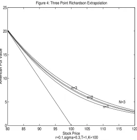
For example, a 3 point Richardson extrapolation can be obtained by assuming that our approximation is approximately quadratic in the mean period length:

^

P

(4)

P

^(0) + ^

P

0(0)

4+ 12 ^

P

00(0)

4 2

:

Substituting in 4=

T

4=

T=

2 and 4=

T=

3 leads to 3 equations in the 3 unknowns ^

P

(0)

P

^

0(0)

and

^

P

00(0). Inverting the system implies that the 3 point extrapolation is given by:

^

P

1:3

(0)

1

2

P

^(

T

);4 ^

P

(

T=

2) + 92 ^

P

(

T=

3)

:

(30)

Figures 4 and 5 illustrate the idea behind a 3 point extrapolation. >From Marchuk and Shaidurov (1983), p. 24, an

N

point Richardson extrapolation is the following weighted12 average of

N

randomized put

values:

^

P

1:N

(0)

N

X

n=1

(;1)N ;n

n

N

n

!(

N

;

n

)!

^

P

(

T=n

)

:

(31)

The critical stock price can be obtained by imposing either of the smooth pasting conditions in (21) or13 by Richardson extrapolation:

S

1:N(0)

N

X

n=1

(;1)N ;n

n

N

n

!(

N

;

n

)!

The eectiveness of Richardson extrapolation is illustrated by a typical test case:

S

= 100

K

= 100

T

= 1

r

= 0

:

1

and

= 0

:

3. The true value based on the binomial method with 2000 time steps appears to be 8.3378. Table 1 shows that for this test case, the unextrapolated values approach the true value very slowly from below. In contrast, the extrapolated put values converge rapidly to this true value, with penny accuracy obtained in only 5 points. Table 2 elaborates on the calculation of the rst two unextrapolated values in Table 1. Besides indicating typical values of some of the variables, it should aid in the reproduction of the results of Table 1.

Broadie and Detemple (1996) and Ju (1997) conduct extensive numerical simulations of a wide array of methods for valuing American options. Both papers conclude that three approaches dominate other methods in terms of speed and accuracy. These three methods are the lower and upper bound approx-imation (LUBA) in Broadie and Detemple (1996), the piecewise exponential boundary approxapprox-imation in Ju (1997), and the randomization approach discussed in this paper. Of these three methods, LUBA has the singular advantage of providing bounds as well as an accurate approximation. The randomiza-tion approach is unique in that the exercise boundary is given by a recursion rather than root nding, when dividends are constant or zero. Finally, Ju's exponential boundary approach appears to deliver the best combination of speed and accuracy, although speed comparisons at each accuracy level were not conducted.

!

5 Extension to Positive Dividends and American Calls

also unable to deal with a linear dividend rate, this section develops formulas for randomized American option values when the dividend payout rate has both a xed and a proportional component. We also show that our approximation to the put's critical stock price is still given by an explicit formula when dividends are constant, but must be determined numerically when there is a proportional component to the dividend ow. Finally, we show how to nd the randomized values of American calls on dividend paying stocks.

We assume that the underlying stock pays dividends continuously until the xed maturity

T

. To obtain a truly xed component

of this dividend ow, we follow Roll (1979) in assuming that this component has been escrowed out of the stock price. In other words, the time

t

stock price

S

t decomposes into:

S

t=

_r

1;

e

;r(T;t)

] +

s

t

t

20

T

]

(33)

where the rst term is the present value at

t

of the constant ow

until

T

, and the residual

s

t is the

stripped price, reecting the stripping o of the xed component of the dividend ow from the stock price. We assume that the risk-neutralized process for the stripped price f

s

t

t

20

T

]g is the following

geometric Brownian motion:

s

t =

s

exp

"

r

;

;

2

2

!

t

+

W

t

#

t

20

T

]

(34)

where f

W

t

t

20

T

]gis a standard Brownian motion, and from (33), the initial value is:

s

=

S

;

r

1;

e

;rT

]

:

(35)

Thus, the dollar dividend rate

d

t has both a xed and a proportional component:

d

t=

+

s

t

t

20

T

]

:

(36)

5.1 Positive Dividends and American Puts

We generalize the previous analysis by letting

P

(

ts

T

) denote the value of an American put as a function of the current time

t

, the current stripped price

s

, and the maturity date

T

. We also dene the critical stripped price

s

(

t

) as the largest stripped price

s

at which the American put value

P

(

ts

T

) equals its exercise value

K

;

s

;r1;

e

;r(T;t)], for

t

20

T

]. From (33), the critical stock price

S

(

t

) is now dened

by:

S

(

t

)

r

1;

e

;r(T;t)

] +

s

(

t

)

t

20

T

]

:

(37)

In the random maturity setting, the underlying stock pays dividends continuously until the option matures. Recalling that

R

1

1+r4 is the discount factor over a single period of random length, the

random maturity analog of (35) is:

s

=

S

;

4(

R

+

R

2+

:::

+

R

n) =

S

;

rR

(1;

R

n)

:

(38)

We dene

P

(m)(

s

) as our approximation for the American put value when

m

random periods remain,

m

= 1

:::n

. Our approximation for the critical stripped price,

s

m, is the largest

s

satisfying

P

(m)(

s

) =

K

;

s

; r

R

(1;

R

m)

m

= 1

:::n:

The values of European options maturing in

n

random-length periods are:

p

(n)(

s

) = 8 > < > : ; sK ; n

;1

P

k=0

(2ln(sK))

k

k!

n;k;1 P l=0 ;n ;1+l n;1

KR

n

_q

n

_p

k+l

;

KD

n

q

^n

p

^k

+l] if

s > K

KR

n;

sD

n+

c

(n)(

S

) if

s

K

(39)

c

(n)(

s

) = 8

>

<

>

:

sD

n;

KR

n+

p

(n)(

s

) if

s > K

;s

K + n

;1

P

k=0

(2ln(Ks))

k

k!

n;k;1 P l=0 ;n ;1+l n;1

KD

n

_p

_^n

_q

_^k+l

;

KR

n

p

n

q

k

+l] if

s

K

(40) where now

1 2 ;r ;

2 ,

R p q

p

^

q

^ are again given by (24) and (10), while:

D

1 1 +

4

:

(41)

For

= 0 and

rK

, American puts are not rationally exercised early. Consequently, the randomized

as:

P

(n)(

s

) = 8

>

<

>

:

p

(n) 0 (

s

) +

b

(n)

1 (

s

) if

s > s

0

K

v

(n)

i (

s

) +

b

(n)

i (

s

) +

A

(n)

i (

s

1) if

s

2(

s

i

s

i

;1]

i

= 1

:::n

K

;

S

if

s

s

n,

(42)

where for

i

= 1

:::n

,

v

(n)

i (

s

) is the randomized value of a short forward position maturing in

n

;

i

+ 1

periods:

v

(n)

i (

s

) =

KR

n;i+1

;

sD

n ;i+1

;

RR

n;i+1 ;

R

n

1;

R

(43)

b

(n)

i (

s

) is the present value of the interest less dividends (net interest) received when below the boundary

for the rst

n

;

i

+ 1 periods:

b

(n)

i (

s

) = n

;i+1 X

j=1

s

s

n;j+1

! ; j

;1

X

k=0

2

ln

s s_n;j+1

k

k

!

j;k;1 X

l=0

j

;1 +

l

j

;1 !

q

j

_p

k+l

R

j

(

Kr

;

);

q

^j

p

^k +l

D

j

s

n;j+1

]

4

(44)

while

A

(n)

i (

s

1) represents the randomized value of a European call less the net interest paid above the

boundary over the complementary period, after accounting for the smoothness at the exercise boundary in every period:

A

(n)

i (

s

h

) = n

;i+1 X

j=h

s

s

n;j+1

! + j

;1

X

k=0

2

ln

s_n;j+1

s

k

k

!

j;k;1 X

l=0

j

;1 +

l

j

;1 !

p

j

_q

k+l

R

j(

Kr

;

);

p

^j

q

^k +l

D

j

s

n;j+1

]

4

:

(45)

Continuity in

s

at the strike price in each period

m

= 1

:::n

again implies

c

(m)

1 (

K

) =

A

(m) 1 (

K

1),

which in turn implies that each critical stripped price

s

m implicitly solves:

c

(m) 1 (

K

)

;

A

(m)

1 (

K

2) =

K

s

m

+

pR

(

Kr

;

);

pDs

^ m

]4

m

= 1

:::n

(46)

where from (40), the at-the-money call value on the left hand side (LHS) of (46) simplies to:

c

(m) 1 (

K

) =

m;1 X

l=0

m

;1 +

l

m

;1 !

KD

m

_p

_^m

_q

_^l

;

KR

It is straightforward to recursively solve (46) numerically for each critical stripped price

s

m, since

s

m

does not appear on the LHS. Setting

= 0 in (46) implies the following explicit solution for the critical stripped prices when the dividend rate is constant at

:

s

m =

K

pR

(

Kr

;

)4

c

(m) 1 (

K

)

;

A

(m) 1 (

K

2)

! 1

+

m

= 1

:::n

(48)

where the call value

c

(m)

1 (

K

) is now given by (28). This solution is a good initial guess when numerically

solving (46). From (38), each critical stock price

S

m is determined by:

S

m =

_rR

(1;

R

m) +

s

m

m

= 1

:::n

(49)

where

s

m is given by (48) when

= 0 and solves (46) otherwise. Letting

S

(4)

S

n denote the initial

critical stock price as a function of the mean period length 4, one can use Richardson extrapolation (32)

to approximate the initial critical stock price for an American put on a dividend paying stock.

5.2 Positive Dividends and American Calls

When there is no xed component to the dividend (i.e.

= 0), an American put call symmetry result can be used to easily value American calls on stocks with a constant dividend yield

. Let

P

(

SK

r

) and

C

(

SK

r

) denote the respective values of American puts and calls with xed maturity

T

. Working in the binomial model, McDonald and Schroder (1990) show that:

C

(

SK

r

) =

P

(

KS

r

)

:

In words, the call value can be obtained from the put valuation formula by switching the stock price and strike price, and also by switching the riskfree rate and dividend yield. This result is proved in the Black Scholes model by Schroeder (1997) and Carr and Chesney (1997), who also prove the corresponding result for critical stock prices:

"

S

(

r

) =

K

2

In words, the critical stock price for an American call can be obtained from that of an American put by switching the riskfree rate and dividend yield, and then obtaining the geometric reection in the strike.

It can be shown that these symmetry results also hold for randomized option values and critical stock prices. Furthermore, randomized American calls can be valued directly when there is also a xed component to the dividend ow. The appendix presents the formulas for the call value and critical stock price in this case.

6 Summary

Appendix

This appendix collects all the formulas needed to calculate random maturity values of European and American puts and calls when the underlying has a continuous payout with a xed component

and a proportional component

. Letting

s

=

S

;

r1;

e

;rT]

the

N

-point Richardson extrapolation of the

randomized European put formula is:

p

1:N(

s

)

N

X

n=1

(;1)N ;n

n

N

n

!(

N

;

n

)!

p

(n)(

s

)

where:

p

(n)(

s

) = 8 > < > : ;s K ; n

;1

P

k=0

(2ln(sK))

k

k!

n;k;1 P l=0 ;n ;1+l n;1

KR

n

_q

n

_p

k+l

;

KD

n

q

^n

p

^k

+l] if

s > K

KR

n;

sD

n+

c

(n)(

s

) if

s

K

(50) and where:

1 2;

r

;

2

4

T

n R

1 1 +

r

4

D

1 1 +

4

s

2+ 2

R

2 4

p

;

2

q

1;

p

p

^

;

+ 1

2 and ^

q

1;

p:

^

The

N

-point Richardson extrapolation of the randomized put formula is

P

1:N(

s

)

N

P

n=1 (;1)N

;nnN

n!(N;n)!

P

(n)(

s

)

where:

P

(n)(

s

) = 8

>

<

>

:

p

(n) 0 (

s

) +

b

(n)

1 (

s

) if

s > s

0

K

v

(n)

i (

s

) +

b

(n)

i (

s

) +

A

(n)

i (

s

1) if

s

2(

s

i

s

i

;1]

i

= 1

:::n

K

;

S

if

s

s

n,

where for

i

= 1

:::nv

(n)

i (

s

) =

KR

n;i+1

;

sD

n ;i+1

;r

R

(

R

n ;i+1

;

R

n)

b

(n)

i (

s

) = n

;i+1 X

j=1

s

s

n;j+1

! ; j

;1

X

k=0

2

ln

s s_n;j+1

k

k

!

j;k;1 X

l=0

j

;1 +

l

j

;1 !

h

q

j

_p

k+l

R

j(

Kr

;

);

q

^j

p

^k +l

D

j

s

n;j+1

i

4

A

(n)

i (

s

h

) = n

;i+1 X

j=h

s

s

n;j+1

! + j

;1

X

k=0

2

ln

s_n;j+1

s

k

k

!

j;k;1 X

l=0

j

;1 +

l

j

;1 !

h

p

j

_q

k+l

R

j(

Kr

)

p

^j

q

^k+l

D

j

s

n j

i

If

= 0, the critical stripped prices are given by

s

m=

K

pR(Kr; )4

c(m) 1

(K);A (m) 1

(K 2) 1

+

m

= 1

:::n:

If

>

0, the critical stripped prices solve:

m;1 X

l=0

m

;1 +

l

m

;1 !

KD

m

_p

_^m

_q

_^l

;

KR

m

_p

m

_q

l_]

;

A

(m)

1 (

K

2) =

K

s

m

+

pR

(

Kr

;

);

pDs

^ m

]4

m

= 1

:::n:

Letting

s

(

T=n

)

s

n denote the solution obtained by recursing on "

s

m, the

N

-point Richardson

extrapo-lation of the put's initial critical stock price is

S

1:N

r1;

e

;rT] +

N

P

n=1 (;1)N

;nnN

n!(N;n)!

s

(

T=n

)

:

Similarly, letting

s

=

S

;

r1;

e

;rT]

the

N

-point Richardson extrapolation of the randomized

European call formula is

c

1:N(

s

)

N

P

n=1 (;1)N

;nnN

n!(N;n)!

c

(n)(

s

)

where:

c

(n)(

s

) = 8

>

<

>

:

sD

n;

KR

n+

p

(n)(

s

) if

s > K

;s

K

+ n

;1

P

k=0

(2ln(Ks))

k

k!

n;k;1 P l=0 ;n ;1+l n;1

KD

n

_p

_^n

_q

_^k+l

;

KR

n

p

n

q

k

+l] if

s

K

(51)

and where again:

1 2;

r

;

2

4

T

n R

1 1 +

r

4

D

1 1 +

4

s

2+ 2

R

2 4

p

;

2

q

1;

p

p

^

;

+ 1

2 and ^

q

1;

p:

^

For

= 0 and

rK

, early exercise is not optimal so the randomized call value is given by (51).

For

>

0 or

> rK

, the

N

point Richardson extrapolation of the randomized call value is

C

1:N(

s

)

N

P

n=1 (;1)N

;nnN

n!(N;n)!

C

(n)(

s

)

where:

C

(n)(

s

) = 8

>

<

>

:

S

;

K

if

s

s

"n

;

v

(n)

i (

s

) +

(n)

i (

s

) +

B

(n)

i (

s

1) if

s

2"

s

i

;1

s

"i)

i

= 1

:::n

c

(n)

0 (

s

) +

(n)

1 (

s

) if

s <

s

" 0

K

where for

i

= 1

:::n

;

v

(n)

i (

s

) =

sD

n;i+1+

r

R

(

R

n;i+1

;

R

n);

KR

n

;i+1 is the initial value of a long

forward position maturing in

n

;

i

+ 1 periods,

(n)

i (

s

) = n

;i+1 X

j=1

s

"

s

n;j+1 !

+ j ;1

X

k=0

2

ln

sn;j+1

s

k

k

!

j;k;1 X

l=0

j

;1 +

l

j

;1 !

h

^

p

j

_q

_^k+l

D

j"

s

n;j+1

;

p

j

q

k

+l

R

j(

Kr

;

)

i

is the initial value of dividends less interest received above the boundary for the rst

n

;

i

+ 1 periods,

while:

B

(n)

i (

s

h

) = n

;i+1 X

j=h

s

"

s

n;j+1 !

; j ;1

X

k=0

2

ln

s

sn;j+1 k

k

!

j;k;1 X

l=0

j

;1 +

l

j

;1 !

h

^

q

j

_p

_^k+l

D

j

"

s

n;j+1

;

q

j

p

k

+l

R

j

(

Kr

;

) i

4

:

B

(n)

i (

s

h

) is the inital value of a European put less the excess of dividends over interest received below the

boundary over the complementary period, after accounting for the smoothness of the exercise boundary in every period. Continuity in

s

at

K

in each period implies that "

s

m solves:

p

(m) 0 (

K

)

;

B

(m)

1 (

K

2) =

K

"

s

m ;

^

qD

s

"m

;

qR

(

Kr

;

)]4

m

= 1

:::n

(52)

where from (50),

p

(m) 0 (

K

) =

m;1 P l=0 ;m ;1+l m;1

KR

m

_q

m

_p

l;

KD

m

q

^m

p

^l]

:

If

=

rK

, (52) can be solved, and

"

s

m =

K

KqD^ 4

p(m) 0

(K);B (m) 1

(K 2)

1

;;1

m

= 1

:::n:

This solution is a good initial guess when solving (52) numerically. Recursively solving for each "

s

m results in "

s

(

T=n

)

s

"n

:

The

N

-point Richardson

extrapolation of the call's critical stock price is "

S

1:N(

T

)

r1;

e

;rT] +

N

P

n=1 (;1)N

;nnN

1. I thank the referee for this insight.

2. However, given the speed of modern computers, they argue that its inherent accuracy makes it the method of choice among those tested.

3. As usual, the rst passage time is considered to be innite if the boundary is never touched.

4. Note that the randomized value obtained in this paper is strictly smaller than the value of an exponentially weighted portfolio of true American puts, i.e.

P

(1)(

S

)

<

R

1

0

e

;t

P

(0

S

t

)

dt

. The

reason is that the optimization over boundaries for our contract must be done with a random maturity. In contrast, the given integral simply averages American values over maturities, where each American value

P

(0

S

t

) is calculated by optimizing over a xed maturity

t

. I thank the editor, Kerry Back, for correcting a mistake on this point in an earlier draft.

5. The Laplace-Carson transform diers from the standard Laplace transform only by the introduction of a constant

in the kernel. See Rubinstein and Rubinstein (1993), pgs. 512{517 for the properties of this transform.

6. Put Call Parity holds so long as the options and a forward contract mature at the same jump time.

7. The binomial model uses a forward nite dierence for the maturity derivative leading to an explicit scheme. The appearance of a backward dierence for the maturity derivative indicates that our randomization procedure may be considered as the limiting case of a fully implicit scheme, where the size of each space step is innitesimally small. Surprisingly, this implicit scheme has a semi-explicit solution for an American option and a fully explicit solution for a European or barrier option.

9. Note that (22) is closely related to the value of a xed maturity American option when the variance rate is gamma distributed. See Madan and Chang (1997) for a closed form solution for European options.

10. See (51) and (50) in the appendix for the randomized values of European calls and in-the-money European puts respectively.

11. This value also accounts for the smoothness at the exercise boundary in every period.

12. The weights always sum to unity and alternate in sign. In general, higher order approximations involve weights with greater absolute value. As a result, implementing higher order extrapolations on a computer requires double precision to control roundo error.

Black, F., and M. Scholes, 1973, \The Pricing of Options and Corporate Liabilities," The Journal of Political Economy, 81, 637{659.

Brennan, M., and E. Schwartz, 1977, \The Valuation of American Put Options," Journal of Finance, 32, 449{462.

Broadie, M., and J. Detemple, 1996, \American Option Valuation: New Bounds, Approximations, and a Comparison of Existing Methods," Review of Financial Studies, 9, 1211-1250.

Carr, P., and M. Chesney, 1997, \American Put Call Symmetry," forthcoming in Journal of Finan-cial Engineering.

Carr, P., and D. Faguet, 1997, \Fast Accurate Valuation of American Options," Cornell University working paper.

Carr, P., R. Jarrow, and R. Myneni, 1992, \Alternative Characterizations of American Put Op-tions," Mathematical Finance, 87{106.

Cass, D., and M. Yaari, 1967, \Individual savings, Aggregate Capital Accumulation, and Ecient Growth," in Essays on the Theory of Optimal Economic Growth, K. Shell ed., Cambridge, MA: MIT Press.

Cox, J., S. Ross, and M. Rubinstein, 1979, \Option Pricing: A Simplied Approach," Journal of Financial Economics, 7, 229{263.

Geske, R., and H. Johnson, 1984, \The American Put Option Valued Analytically," Journal of Finance, 39, 1511{1524.

Huang, J, M. Subrahmanyam, and G. Yu, 1996, \Pricing and Hedging American Options: A Recursive Integration Method", Review of Financial Studies, 9, 277-300.

Jacka, S. D., 1991, \Optimal Stopping and the American Put," Mathematical Finance, 1, 1-14.

Jamshidian, F., 1989, \Formulas for American Options," Merrill Lynch Capital Markets working paper.

Ju, N., 1997, \Pricing an American Option by Approximating Its Early Exercise Boundary As a Multi-Piece Exponential Function," University of California, Berkeley working paper.

Kim, I. J., 1990, \The Analytic Valuation of American Puts," Review of Financial Studies, 3, 547{572.

Leisen, D., 1997, \The Random-Time Binomial Model," University of Bonn working paper.

McKean, Jr., H. P., 1965, \Appendix: A Free Boundary Problem for the Heat Equation Arising from a Problem in Mathematical Economics," Industrial Management Review, 6, 32{39.

Madan, D., and E. Chang, 1997, \The Variance Gamma Option Pricing Model," University of Maryland working paper.

Marchuk, G., and V. Shaidurov, 1983, Dierence Methods and Their Extrapolations, Springer Ver-lag, NY.

McDonald, R., and M. Schroder, 1990, \A Parity Result for American Options," Northwestern University working paper.

Merton, R. C., 1973, \Theory of Rational Option Pricing," Bell Journal of Economics and Man-agement Science, 4, 141{183.

Meyer, G. H., 1970, \On a Free Boundary Problem for Linear Ordinary Dierential Equations and the One-Phase Stephan Problem," Numerical Mathematics, 16, 248{67.

Meyer, G. H., 1979, \One-Dimensional Free Boundary Problems," SIAM Review, 19, 17{34.

Meyer, G. H., and J. van der Hoek, 1994, \The Evaluation of American Options with the Method of Lines," Georgia Institute of Technology working paper.

Rektorys, K., 1982, The Method of Discretization in Time and Partial Dierential Equations, D. Reidel Publishing Co., Dordrecht-Boston, MA.

Rendleman R., and B. Bartter, 1979, \Two-State Option Pricing," Journal of Finance, 34, 1093-1110.

Rogers, C., and E. Stapleton, 1997, \Fast Accurate Binomial Pricing," forthcoming in Finance and Stochastics.

Roll, R., 1977, \An Analytic Valuation Formula for Unprotected American Call Options on Stocks with Known Dividends," Journal of Financial Economics, 5, 251{58.

Rothe, E., 1930, \Zweidimensionale parabolische Randwertaufgaben als Grenzfall eindimensinaler Randwerttaufgaben,"Math. Ann. 102.

Rubinstein, I., and L. Rubinstein, 1993, \Partial Dierential Equations in Classical Mathematical Physics," Cambridge University Press.

Schroeder, M., 1997, Results on Futures, Forwards, and Options Obtained Using a Change of Numeraire," working paper SUNY-Bualo.

Table 1: Convergence of Randomized Put Value to American without and with Richardson Extrapolation

S = 100, K = 100, T = 1, r = 0.1,

= 0,

= 0

:

3

Number of Steps

n

or Points

N

Unextrapolated Put Value

P

(n) Extrapolated Put Value

P

1:N

1 7.0405 7.0405

2 7.6175 8.1946

3 7.8353 8.3089

4 7.9505 8.3257

5 8.0220 8.3311

6 8.0709 8.3333

7 8.1065 8.3345

8 8.1335 8.3353

9 8.1548 8.3358

10 8.1720 8.3362

11 8.1862 8.3365

12 8.1981 8.3367

13 8.2082 8.3369

14 8.2169 8.3370

Table 2: Intermediate Put Values

Variable n=1 n=2

4 1.0000 0.5000

-0.6111 -0.6111

R

0.9091 0.9524

4.9818 6.8586

p

0.5613 0.5446

q

0.4387 0.4554 ^

p

0.6617 0.6175 ^

q

0.3383 0.3825

S

1 77.9724 80.7216

S

2 N/A 77.2941

v

(n)

1 (

S

) -9.0909 -9.2971

b

(n)

1 (

S

) 0.9917 1.0176

A

(n)

1 (

S

1) 15.1397 15.8970

50 60 70 80 90 100 110 120 130 140 150 5

10 15 20 25 30 35 40 45 50

Randomized Put Value

[image:35.612.59.343.266.546.2]

Stock Price

Figure 1: Value of Exponential Maturity Put

r=0.1,sigma=0.3,K=100,T=1.0,n=1

0 0.5 1 1.5 2 2.5 3 0

0.2 0.4 0.6 0.8 1

Probability Density

[image:36.612.59.319.265.540.2]

Calendar Time (years)

Figure 2: Convergence of Gamma Density Functions

Pdf(1)

Pdf(2)

Pdf(3)

0 0.1 0.2 0.3 0.4 0.5 0.6 0.7 0.8 0.9 1 75

80 85 90 95 100 105

Critical Stock Price

[image:37.612.56.336.261.553.2]

Calendar Time (years)

Figure 3 Exercise Boundary of Erlang Maturity Put

Strike Price

r=0.1,sigma=0.3,T=1,K=100,T01=.53,T12=.40

80 85 90 95 100 105 110 115 120 0

5 10 15 20 25

N=3

American Put Value

[image:38.612.61.342.263.550.2]

Stock Price

Figure 4: Three Point Richardson Extrapolation

n=1 n=2 n=3

r=0.1,sigma=0.3,T=1,K=100

0 0.1 0.2 0.3 0.4 0.5 0.6 0.7 0.8 0.9 1 0

1 2 3 4 5 6 7 8

[image:39.612.59.342.266.549.2]

8.336 Figure 5: Three−step Richardson Extrapolation

American Put Value

Calendar Time (years)

7.04 7.618 7.835

r=0.1,sigma=0.3,T=1,K=100