COMPARISON OF BLIND SOURCE SEPARATION ALGORITHMS FOR MIXED IMAGES

(1)

Available Online at www.ijpret.com 1149

INTERNATIONAL JOURNAL OF PURE AND

APPLIED RESEARCH IN ENGINEERING AND

TECHNOLOGY

A PATH FOR HORIZING YOUR INNOVATIVE WORK

COMPARISON OF BLIND SOURCE SEPARATION ALGORITHMS FOR MIXED

IMAGES

AJIT B. PANDE1, MILIND PARAYE2, MONIKA WADHAI3

1.Assistant Professor, Department of Electronics and Tele-communication Engineering, IBSS College of Engineering, Amravati. 2.Assistant Professor, Department of Electronics and Tele-communication Engineering, Sardar Patel Institute Of Technology, Mumbai. 3.Assistant Professor, Department of Electronics and Tele-communication Engineering, Ramrao Adik Institute Of Technology, Navi Mumbai

Accepted Date: 05/03/2015; Published Date: 01/05/2015

\

Abstract: In this paper the independent component analysis (ICA) algorithm, Infomax algorithm was studied and compares the performances of this two algorithms. Then, carried out simulation in blind sources process of the mixing images. Through simulation of three color images mixed by a random matrix, and using the Fast ICA separation algorithm and Infomax Algorithm, original images retrieved from the mixed images. The simulation result using MATLAB shows better performance of image separation using Fast ICA algorithm and execution time (elapsed time) is very less than InfoMax Algorithm. Performance parameters like Peak Signal to Noise Ratio (PSNR), Root Mean Square Error (RMSE) are used to evaluate quality of separated images.

Keywords: Blind source separation, ICA, random matrix, mixing images, Fast ICA, Infomax.

.

Corresponding Author: MR. AJIT B. PANDE

Access Online On:

www.ijpret.com

How to Cite This Article:

Ajit B. Pande, IJPRET, 2015; Volume 3 (9): 1149-1157

(2)

INTRODUCTION

At present, the blind signal separation (BSS) [1] in signal processing field has got more and more attention because in the wireless communication, medical analysis, speech recognition, image processing field, it has broad prospect of application. In the past ten years. BSS problem is to separate independent signal source from linear mixing signals in the premise without prior knowledge based on the statistical independent theory, which can also called the independent component analysis. [2] Since J.H erault and Jutten [3] first carried out research of BSS, and a lot of scholars BSS problem carried on a series of research, at present BSS method has put forward a series of algorithm. These methods of the signal processing have been widely applied on many fields, but in the image blind source separation, the discussed algorithm has little research.[4].

2. Blind Source Separation Algorithms

The BSS algorithms studied in this paper are the FastICA and Infomax algorithms.

2.1 FastICA Algorithm

2.1.1 Independent Component Analysis

The aim of ICA is that n dimension signals decompose into a set of linear combination of

statistical independent random variable. Suppose that x1(t), x2(t),….., xn(t) are n dimension.

Observed random variable, and they are the linear combination of n unknown source signal,

s1(t),…,sn(t) . Assume, x(t) = [x1(t),….., xn(t)]T, s(t) = [s1(t),…,sn(t)]T after they are combined with

the linear mixed system A,they can be expressed by

𝑥₁ = 𝑎_𝑖𝑗

𝑁

𝑗 =1

𝑠_𝑗 𝑡 ; 𝑖 = 1, … , 𝑁 (1)

Equation (1) is written as

𝑋 𝑡 = 𝐴𝑠 𝑡 (2)

Where, A = [a1 , …. , an] is non-singular mixed matrix. Given that each s j(t) is mutual independent and the problem that ICA will solve is to estimate unknown independent source

s(t) through another mixed matrix B in terms of observed data x(t). Sometimes, the solving

mixed system B is decomposed into two steps: one is that the observed vector x(t) transforms

(3)

component of z(t) is demanded to be orthogonality and normalization, furthermore, all

variances are 1. Equation is written by

𝑧 𝑡 = 𝑊𝑥 𝑡 , 𝐸[𝑧 𝑡 𝑧𝑇 𝑡 = 𝐼_𝑁… … . . (3)

In fact, the first step is called sphering (also called whitening or normalization decorrelation).

The purpose of sphering is to make all variances of each component zi(t) of output variable Z(t)

be 1, and they are incorrelate but not always mutual independence. The second step is

orthogonal transform, whose aim is to make each component yi(t) as much as possible mutual

independent.

ICA is an optimization computational problem under some criterions, namely, how to make separated independent components approach each source signal as much as possible. So the problem includes two aspects: 1) Adopting a criterion acts as the rule to judge a set of signal whether or not near mutual independent; 2) Using an algorithm realizes this aim.

In the course of learning ICA algorithm, an objective function (optimization criterion) J (W) with

W as variable unit is founded by information’s and statistics methods. If some

can make J (W) reach maximum or minima value, is the solution, then seek an effective and

speedy algorithm to solve . The typical algorithms include random gradient method, nature gradient method, fixed-point algorithm. ICA fixed-point algorithm has faster convergence speed than batch processing, even adaptive processing algorithm, which is called fast ICA algorithm.

2.1.2 FastICA Algorithm analysis

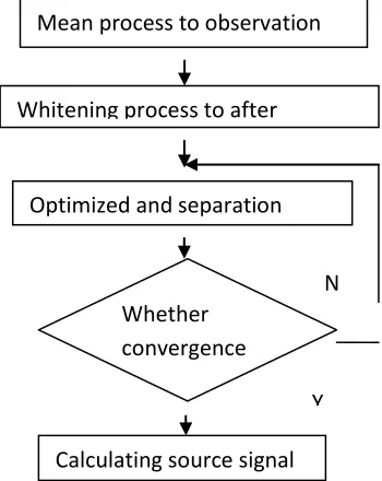
The realization of Fast ICA algorithm includes three points, the first, removing mean value of the observation signal, the second, whitening processing to the observation signal after mean processing, the third, the process of independent components extraction algorithm and realization. Algorithm realization flow is shown as Figure 1. The first two steps can be regarded as the pretreatment to the observation signal. Through mean and whitening processing, ICA algorithm process can be simplified.[9]

The specific procedure is shown as follows:

(1) Inputing mixing signal X;

(2) Meaning the obversation data X and making the mean value is 0;

(4)

(4) Choosing the need to assess the number of components, set Iteration times p←1;

(5) Randomly selecting chosen initialized weights vector woand k = 0;

(6) 𝑤_𝑘+1 = 𝑤_𝑘 − 𝐸 {𝑥𝑔 𝑤𝑘𝑇𝑥 − 𝛽𝑤𝑘 𝐸{ 𝑔′_𝑤

𝑘𝑇𝑥 − 𝛽

(4)

Using above formula to update weights vector

w k+1. Where 𝛽 = 𝐸{𝑥𝑔(𝑤_𝑘𝑇𝑥)}

(7) Normalized w K+1 and

𝑤𝑘+1= 𝑤𝑘+1 _||𝑤

𝑘+1|| ;

(8) If 𝑤_𝑘+1 − 𝑤_𝑘 > 𝜀 , then the algorithm is not convergence, return to step (2), or Fast ICA

algorithm estimate a independent component, and the algorithm is over. For many numbers independent component extraction, we can repeat to use above basic form of FastICA algorithm. To be sure each time’s different components extracted, we only need to remove independent component having be extracted from the observation signal in every times, and repeat this process until all the dependent components needed to be extracted.

Figure 1. Flow diagram of FastICA Algorithm. Mean process to observation

signal

Optimized and separation matrix

Whether convergence ?

Whitening process to after meaning signal

Calculating source signal N

(5)

2.2 InfoMax Algorithm

The information maximization(InfoMax) algorithm (often known as infomax) developed by Bell and Sejnowski [1] catalysed a surge of interest in using information theory to perform blind source separation. In 1995, Bell and Sejnowski proposed an adaptive learning algorithm that maximizes the information passed through neural networks. The paper shows that a neural network is capable of resolving the independent components in the inputs, that is, the neural network can perform independent component analysis. The main idea is that maximizing the joint entropy H(y) of the outputs of a neural processor can approximately minimize the mutual information among the output components. The joint entropy of n variable,y1,y2,y3 (Assume they are the outputs of a neural network) may be written as:

H(y1,…,yn) – H(y1)+H(yn)-I(y1,…,yn) (1)

If the nonlinear transfer function of a neural network matches the probability density function of the inputs and the joint entropy H(y1,….,yn)of the outputs is maximized, the mutual information I(y1,…,yn) among the outputs is then minimized. The output signals are assumed to be independent. Bell and Sejnowski noted that many real-world analog signals including the speech signals are super-gaussian and satisfies the independence condition assumed if the transfer function of the neurons in the neural network is a sigmoidal or hyperbolic tangent function.

The learning rule for a single layer feedforward neural network to implement the separation is

∆𝑊 ∝ [𝑊𝑇]−1+ 1 − 2𝑦 𝑥𝑇 (2)

∆ 𝑤₀ ∝ 1 − 2𝑦 (3)

Where 𝑦 = 𝑓(𝑊𝑥 + 𝑤0) and 𝑓(𝑢) Is a sigmoid contrast function , usually 𝑓 𝑢 − 1 + 𝑒−𝑢 −1

or 𝑓 𝑢 − tanh 𝑢 .

A similar learning algorithm was derived by Amari etc [5] using the natural gradient in the

parameter space insteadof the descent gradient. This learning rule is :

∆ 𝑊 ∝ 1 − 𝑓 𝑢 . 𝑢𝑇 . 𝑊

Where 𝑓 𝑥 = 3

4𝑥

11₊25

4 𝑥

9₋14

3 𝑥

7₋47

4 𝑥

5₊29

4 𝑥

3_{. This rule speeds up the algorithm by}

(6)

(i) Root mean square error (RMSE): Root mean square value is calculated by taking the square root of mean square error(MSE).

𝑅𝑀𝑆𝐸 = 1

𝑀𝑁 (𝐼𝑖𝑗 − 𝐼 𝑖𝑗)2

𝑀

𝑗 =1 𝑁

𝑖=1

Where N × M = Image size, Iij = Original source image, 𝐼 ij = Separated image.

(ii) Peak signal to noise ratio (PSNR): Peak Signal-to-Noise Ratio is the ratio between the

original signal and the separated signal in an image, given in decibels. The higher the PSNR, the closer the separated image is to the original. In general, a higher PSNR value should correlate to a higher quality image.

𝑃𝑆𝑁𝑅 = 20𝑙𝑜𝑔₁₀ ( 255

𝑅𝑀𝑆𝐸)𝑑𝑏

5.2 Algorithm Simulation

(7)

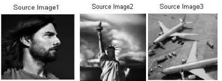
Fig 2.Source Images.

Figure 3. Mixed Images

Figure 4 Separated Images Using Infomax Algorithm.

Figure 5. Separated Images Using FastICA Algorithm.

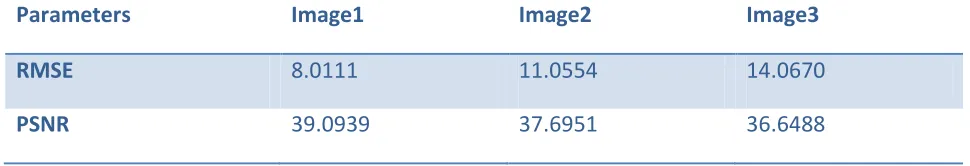
Table 1. Performance parameters for InfoMax Algorithm

Parameters Image1 Image2 Image3

RMSE 8.0111 11.0554 14.0670

PSNR 39.0939 37.6951 36.6488

Table 2. Performance parameters for FastICA Algorithm

Parameters Image1 Image2 Image3

RMSE 6.7401 10.7229 14.0295

(8)

Table 3.Execution speed using Infomax Algorithm and FastICA Algorithm.

Algorithm Execution Speed (Seconds)

InfoMax 4.703027

FastICA 0.075699

The gaussian nonlinear function used to perform ICA, which resulted in faster convergence and minimum distortion in the separated source images.

CONCLUSIONS

This paper gives detailed study of FastICA algorithm, and through the simulation, the set of images that are successfully mixed. The input to the FastICA (Fast-Independent Component Analysis) algorithm known as fixed point algorithm will be mixed images. The original images will then be retrieved using fixed point algorithm known as FastICA algorithm. FastICA algorithm is implemented in MATLAB for the mixed image separation. And various performance parameters calculated to evaluate the quality of separated images. It is observed from Table 1 and Table 2 that, the blind source separation using FastICA Algorithm results in better source separation with minimum distortion in terms of RMSE and PSNR as compared to InfoMax Algorithm. Table 3 confirms the faster convergence of FastICA Algorithm as compare to the Infomax Algorithm.

REFERENCES

1. Guan weihua, Li lifu, Lin yongman, “Underdetermined Blind Separation Algorithm Base d on

Subtractive Clustering”, AISS: Advances in Information Sciences and Service Sciences, Vol. 3, No. 7, pp. 75- 81, 2011.

2. Chengfan LI, Jingyuan YIN, Junjuan ZHAO, Feiyue YE, "Detection and Compensation of

Shadows based on ICA Algorithm in Remote Sensing Image", No. 7, pp. 46-54, 2011.IJACT : International Journal of Advancements in Computing Technology, Vol. 3,

3. Wang Lei, “Research of BSS Method Based on ICA”, Lanzhou University of technology, 2010.

4. Bi Yang, “Research and Application of BSS Algorithm Based on Fast ICA”, Xian university of

(9)

5. Huang Liyan, Gao Qiang, Kang Haiyan, Zhao Zhenbing, Xu Yixi, “Improved Fast ICA

algorithm”, Journal of North China Electric Power Univenity, Vol. 5, pp.59-60, 2006.

6. Yang F. S., Hong B., “ Theory and application of independent component analysis”, Beijing:

tsinghua university press, (2006).

7. Cao Huirong, Zhang Baolei, Ma Li, “The Separation of Mixed Images Based on Fast ICA

Algorithm”, Computer Study, Vol.1, pp. 45, 2004.

8. Hyvarinen A., et al. “Independent component analysis”, John Wiley and Sons, (2001).

9. ARIE Y, “Blind source separation via the second characteristic function”, Signal Processing,

Vol. 80, pp. 897-902, 2000.

10.Hyvarinen A., Oja E., “Independent component analysis: algorithm and application”, Neural

Network, 13(4-5), 411-430, (2000).

11.Comon P, “Independent Component Analysis a New Concept”, Signal Processing, Vol. 36,