www.geosci-model-dev.net/8/363/2015/ doi:10.5194/gmd-8-363-2015
© Author(s) 2015. CC Attribution 3.0 License.
MetUM-GOML1: a near-globally coupled
atmosphere–ocean-mixed-layer model
L. C. Hirons, N. P. Klingaman, and S. J. Woolnough
National Centre for Atmospheric Science-Climate and Department of Meteorology, University of Reading, P.O. Box 243, Reading, Berkshire, RG6 6BB, UK
Correspondence to: L. C. Hirons ([email protected])
Received: 6 August 2014 – Published in Geosci. Model Dev. Discuss.: 24 September 2014 Revised: 22 December 2014 – Accepted: 27 January 2015 – Published: 19 February 2015
Abstract. Well-resolved air–sea interactions are simulated in a new ocean mixed-layer, coupled configuration of the Met Office Unified Model (MetUM-GOML), comprising the Me-tUM coupled to the Multi-Column K Profile Parameteriza-tion ocean (MC-KPP). This is the first globally coupled sys-tem which provides a vertically resolved, high near-surface resolution ocean at comparable computational cost to run-ning in atmosphere-only mode. As well as being computa-tionally inexpensive, this modelling framework is adaptable – the independent MC-KPP columns can be applied selec-tively in space and time – and controllable – by using temper-ature and salinity corrections the model can be constrained to any ocean state.
The framework provides a powerful research tool for process-based studies of the impact of air–sea interactions in the global climate system. MetUM simulations have been performed which separate the impact of introducing inter-annual variability in sea surface temperatures (SSTs) from the impact of having atmosphere–ocean feedbacks. The rep-resentation of key aspects of tropical and extratropical vari-ability are used to assess the performance of these simula-tions. Coupling the MetUM to MC-KPP is shown, for exam-ple, to reduce tropical precipitation biases, improve the prop-agation of, and spectral power associated with, the Madden– Julian Oscillation and produce closer-to-observed patterns of springtime blocking activity over the Euro-Atlantic region.
1 Introduction
Interactions between the atmosphere and ocean are a key feature of Earth’s climate system, from instantaneous ex-changes of heat, moisture and momentum to multi-decadal variability in large-scale, coupled circulations. By modifying the magnitude and direction of radiative and turbulent air– sea fluxes, variations in sea surface temperature (SST) can influence weather and climate globally (e.g. Sutton and Hod-son, 2003; Giannini et al., 2003). However, it is not only in-teractions at the ocean surface which influence climate. The slower adjustment timescales within the upper ocean pro-vide a source of predictability on seasonal timescales (e.g. the El Niño–Southern Oscillation (ENSO); Neelin et al., 1998), and basin-scale circulations within the deep ocean can drive multi-decadal variations in climate (Sutton and Hod-son, 2005).
1.1 The importance of air–sea interactions for weather and climate extremes
1.1.1 Air–sea interactions in the tropics
The dominant mode of subseasonal variability in the tropi-cal atmosphere is the MJO (Madden and Julian, 1971), com-prising eastward-propagating active and suppressed phases of convection in the tropical Indo-Pacific. The interaction between the atmosphere and ocean has been shown to in-fluence the propagation of the MJO in an atmospheric gen-eral circulation model (AGCM) coupled to an idealised slab (e.g. Benedict and Randall, 2011) or a full dynamical ocean (e.g. DeMott et al., 2014) as well as in observations (Shin-oda et al., 2013). Within the tropics, SST anomalies exhibit a near-quadrature phase relationship with rainfall: the peak warm (cold) SST leads the peak in enhanced (suppressed) convection by 7–10 days (Fu et al., 2003; Vecchi and Har-rison, 2002). By inducing moistening downstream, this re-lationship is thought to be important for the propagation of organised tropical convection. However, AGCMs strug-gle to capture this observed phase relationship, often ex-hibiting collocated SST and rainfall anomalies (Rajendran et al., 2004). The observed near-quadrature phase relation-ship is reproduced in a coupled system (Rajendran and Ki-toh, 2006), and results in a better simulation of the MJO (e.g. Woolnough et al., 2007; DeMott et al., 2014) as well as the northward-propagating Boreal summer intraseasonal oscilla-tion (BSISO; e.g. Seo et al., 2007; Wang et al., 2009).
Air–sea interactions and the MJO also influence the on-set and intraseasonal variability in the Asian (e.g. Lawrence and Webster, 2002), Australian (e.g. Hendon and Liebmann, 1990) and West African (e.g. Matthews, 2004) monsoons. For the Asian summer monsoon, the magnitude and gradi-ents of SSTs in the Bay of Bengal and Indian Ocean are key to the formation of the onset vortex over the ocean which in-tensifies and moves northwards as the monsoonal circulation over land (Wu et al., 2012). Anomalous convection associ-ated with the northward-propagating BSISO influences the active-break cycle of the Asian monsoon (e.g. Vitart, 2009; Klingaman et al., 2011). In the Australian pre-monsoon sea-son, trade easterlies support a positive feedback between wind and SST resulting in strong persistent SST anoma-lies north of Australia. The monsoonal westerly regime, which is modulated by the propagation of the MJO active phase through the maritime continent (MC), causes this pos-itive feedback to break down, weakening the SST anoma-lies significantly (Hendon et al., 2012). Oceanic warming around Africa can cause deep convection to migrate over the ocean, weakening the continental monsoon and leading to widespread drought from the Atlantic coast of western Africa to Ethiopia (Giannini et al., 2003). Equatorial warm pool SST anomalies associated with the MJO result in enhanced mon-soonal convection over western and central Africa by
forc-ing eastward-propagatforc-ing Kelvin and westward-propagatforc-ing Rossby waves (Lavender and Matthews, 2009).
As well as influencing seasonal–subseasonal variability, air–sea interactions are key in determining the frequency and intensity of extreme events. Tropical cyclones, for example, are a strongly coupled phenomenon: they extract energy from the ocean and provide oceanic momentum, in the form of up-welling, which results in a cooling of the ocean surface be-low the cyclone centre. Ocean–atmosphere coupling in gen-eral circulation models (GCMs) has been shown to improve the spatial distribution of cyclogenesis (e.g. Jullien et al., 2014), as well as the representation of cyclone intensity (e.g. Sandery et al., 2010).
1.1.2 Air–sea interactions in the extratropics
There is also evidence that local high-frequency SST anoma-lies affect subseasonal variability in the extratropics. By al-tering meridional SST gradients, local anomalous SST pat-terns can affect the baroclinicity of the extratropical atmo-sphere (e.g. Nakamura and Yamane, 2009), resulting in per-sistent blocking conditions, intense heatwaves and droughts. For example, extreme heatwaves in southern Australia are typically induced and maintained by a blocking anticyclone that originates in the western Indian Ocean. An increased meridional SST gradient in the Indian Ocean, and hence enhanced baroclinicity, amplify upper-level Rossby waves which trigger heatwave conditions (Pezza et al., 2012). In summer 2003, warm SST anomalies in the northern Atlantic Ocean reduced the meridional SST gradient and decreased baroclinic activity, resulting in a northward shift of the po-lar jet and an expansion of the anticyclone and leading to an extreme heatwave over Europe (Feudale and Shukla, 2011). However, remote warm SST anomalies in the tropical At-lantic associated with anomalously wet conditions in the Caribbean Basin and the Sahel have also been suggested as a forcing for the 2003 heatwave (Cassou et al., 2005).
1.1.3 Tropical–extratropical teleconnections
1.1.4 Frequency of air–sea interactions
The atmosphere and upper ocean interact instantaneously but many GCMs are only coupled once per day. Introducing diur-nal coupling increases the variability in tropical SSTs which improves the amplitude of ENSO (Ham and Kug, 2010), causes an equatorward shift of the ITCZ (intertropical con-vergence zone) and a resulting stronger and more coherent MJO (Bernie et al., 2008), and improves the northward prop-agation of the BSISO (Klingaman et al., 2011). The impacts of subdaily coupling are not confined to the tropics but can affect the extratropics: including the ocean diurnal cycle de-creased the meridional SST gradients in the North Atlantic resulting in a decrease in the zonal mean flow in the region (Guemas et al., 2013).
It is clear that interactions between the atmosphere and the ocean are important to a wide range of phenomena spanning many spatial and temporal scales. Section 1.2 will examine the current approaches to modelling air–sea interactions in global simulations.
1.2 Air–sea coupling in global climate models
Current widely used approaches for global simulations of climate are (1) AGCMs forced by prescribed SST and sea ice; (2) slab ocean experiments: an AGCM coupled to a sim-ple one-layer thermodynamic ocean with either prescribed or interactive sea ice; and (3) coupled atmosphere–ocean gen-eral circulation models (AOGCMs) run with a full dynam-ical ocean and dynamic sea ice. Each approach has notable advantages and disadvantages. While (1) is computationally inexpensive and requires only an AGCM in which the de-sired SSTs and sea ice can be prescribed, the SST and ice boundary conditions cannot respond to variability in the at-mosphere. This results in the wrong phase relationship be-tween SST and rainfall anomalies (Fu et al., 2003; Rajendran and Kitoh, 2006) and can also lead to significant errors in the representation of phenomena for which air–sea interactions may be a critical mechanism (e.g. the MJO; Crueger et al., 2013).
In (2), the addition of a slab ocean permits thermodynamic processes to occur in the ocean. However, the slab ocean is not vertically resolved but typically comprises an O(50 m) thick layer. The SST response in slab models is often muted due to the slab’s large thermal capacity and constant mix-ing depth. Studies have shown that fine upper-ocean verti-cal resolution allows coupled models to accurately represent subseasonal variations in mixed-layer depth and SST, which in turn enhances tropical subseasonal variability in convec-tion and circulaconvec-tion (Woolnough et al., 2007; Klingaman et al., 2011; Tseng et al., 2014). Therefore, tropical subsea-sonal variability in a slab ocean model is very sensitive to the choice of mixing depth (e.g. Watterson, 2002). For ex-ample, slab ocean models with a very shallow (2 m) mix-ing depth have been shown to have a poor representation of
the MJO: the fast response of the atmosphere disables the wind-induced surface heat exchange (WISHE) mechanism (Maloney and Sobel, 2004). Furthermore, observations have shown that temperature and salinity anomalies stored be-neath the mixing depth can reemerge and influence the atmo-spheric circulation in subsequent seasons (e.g. in the North Atlantic Bhatt et al., 1998; Alexander et al., 2000; Cassou et al., 2007). This mechanism is not present in a slab-coupled ocean model where the mixing depth cannot dynamically evolve.
In (3), both ocean dynamic and thermodynamic processes are represented so there is often no need to prescribe oceanic heat transports. However, the horizontal and vertical resolu-tion of the AOGCM is limited by the computaresolu-tional expense of the ocean, especially if climate-length integrations are re-quired. Furthermore, such models require long spin-up peri-ods to attain a balance within the coupled system. They can also exhibit significant drifts and biases in the mean state, which can be of equal magnitude or larger than the desired signal (e.g. ENSO, decadal ocean variability, responses to greenhouse-gas or aerosol forcing). For example, many cou-pled models have a large cold equatorial SST bias in the trop-ical Pacific which inhibits their ability to simulate key modes of variability such as ENSO (Vannière et al., 2012).
1.3 Motivation for this study
Each of the modelling approaches described above is valu-able and each, depending on the context, can be the most appropriate approach to answer a given set of scientific ques-tions. However, there is a gap in the current modelling capa-bility described in Sect. 1.2: no coupled system can provide a high-resolution, vertically resolved ocean at limited compu-tational cost. The modelling framework described here ad-dresses this gap.
This alternative approach is to couple an AGCM to a mixed-layer thermodynamic ocean model, comprised of one oceanic column below each atmospheric grid point. Previ-ously, this has only been done in a handful of studies which do not use a contemporary AGCM, for example, studies cou-pling the Community Atmospheric Model version 2 (CAM2) to a 1-D ocean (e.g. Bhatt et al., 1998; Alexander et al., 2000; Cassou et al., 2007; Kwon et al., 2011). In this framework, because there is no representation of ocean dynamics, the mixed-layer model is computationally inexpensive (<5 % of the cost of the atmosphere, as measured by CPU time1), which allows for higher near-surface vertical resolution and hence better-resolved upper-ocean vertical mixing than ap-proach (2) and, in many cases, (3).
1The supercomputer used did not allow sharing one node
Therefore, within this coupled framework, well-resolved air–sea interactions are incorporated at comparable compu-tational expense to approaches (1) and (2) but significantly cheaper than (3). This allows climate-length coupled inte-grations to be carried out at much higher atmospheric and oceanic horizontal resolutions than those currently achiev-able with (3).
One notable caveat of this framework is that temperature and salinity corrections must be prescribed, as in (2). While coupling to a mixed-layer model allows thermodynamic pro-cesses to occur in the ocean, corrections of temperature and salinity must be prescribed to represent the mean advection in the ocean and to correct for biases in AGCM surface fluxes. The method used to calculate and apply these correc-tions in this framework is described in Sect. 2.1.1. A further consequence of the lack of ocean dynamics is that the cou-pled model cannot represent modes of variability that rely on dynamical ocean processes (e.g. ENSO, AMO, PDO). How-ever, depending on the application, this controllable feature of the framework could also be considered as an advantage. By adjusting the temperature and salinity corrections, the model can be easily constrained to any desired ocean state. When constrained to observations, for example, this results in much smaller mean SST biases compared with (3) (Fig. 1). This is important because the mean state is known to affect modes of variability (e.g. the MJO; Inness et al., 2003; Ray et al., 2011) and the perceived impact of coupling on that variability (Klingaman and Woolnough, 2014). Within this framework the role of air–sea interactions can be studied in a coupled model with the “right” basic state, thus, limiting the possibility that changes in the variability are a consequence of changes to the mean state. This feature of the coupled modelling system need not only be used to constrain to an observed ocean state, but could be exploited in further sensi-tivity studies (see discussion in Sect. 5).
As well as being controllable, this mixed-layer, coupled modelling framework has further technical advantages. It is very flexible: because the ocean comprises independent columns below each atmospheric grid point, air–sea coupling can be selectively applied in space and time. This provides a test bed for sensitivity studies to understand the relative role of local and remote air–sea interactions and how they feed back onto atmospheric variability. Furthermore, the frame-work is very adaptable: the coupling can be applied to any GCM at its own resolution.
The coupled atmosphere–ocean-mixed-layer model con-figuration, and the simulations which have been performed, are described in Sect. 2. The impact of well-resolved air–sea interactions are evaluated within those simulations in terms of the mean state (Sect. 3) and aspects of tropical (Sect. 4.1) and extratropical (Sect. 4.2) variability. These results are summarised in Sect. 5 along with a discussion of potential further applications of this modelling capability.
0 30E 60E 90E 120E 150E 180 150W 120W 90W 60W 30W 0
Difference in ANNUAL clim SST for K-O minus Obs (1980-2009)
-2.2 -1.8 -1.4 -1.0 -0.6 -0.2 0.2 0.6 1.0 1.4 1.8 2.2
(K)
0 30E 60E 90E 120E 150E 180 150W 120W 90W 60W 30W 0
0 30E 60E 90E 120E 150E 180 150W 120W 90W 60W 30W 0
Difference in ANNUAL clim SST for MetUM-NEMO minus Obs (1980-2009)
-2.2 -1.8 -1.4 -1.0 -0.6 -0.2 0.2 0.6 1.0 1.4 1.8 2.2 (K)
0 30E 60E 90E 120E 150E 180 150W 120W 90W 60W 30W 0
0 30E 60E 90E 120E 150E 180 150W 120W 90W 60W 30W 0
Difference in ANNUAL clim SST for MetUM-NEMO minus Obs (1980-2009)
-2.2 -1.8 -1.4 -1.0 -0.6 -0.2 0.2 0.6 1.0 1.4 1.8 2.2
(K)
0 30E 60E 90E 120E 150E 180 150W 120W 90W 60W 30W 0
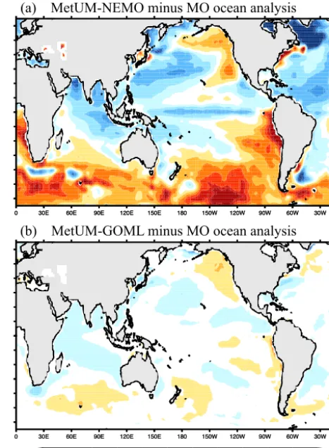
(a) MetUM-NEMO minus MO ocean analysis
(b) MetUM-GOML minus MO ocean analysis
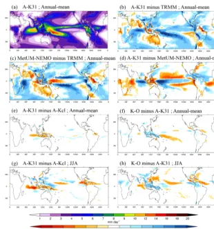
Figure 1. Annual-mean SST bias compared with the Met Office
(MO) ocean analysis (Smith and Murphey, 2007). (a) 30 years of the Met Office Unified Model AGCM (MetUM) coupled to a full dynamical ocean, NEMO. (b) 60 years of a free-running MetUM-GOML simulation: the MetUM coupled to the multi-column mixed-layer ocean model, MC-KPP. The flux corrections in this MetUM-GOML simulation are calculated as described in Sect. 2.2.
2 Model, methods and data
The near-globally coupled atmosphere–ocean-mixed-layer model is described here, first in terms of the general frame-work (Sect. 2.1) and then the specific implementation of that framework to the Met Office Unified Model, as used for the experiments in this study (Sect. 2.2).
2.1 The new coupled modelling framework
MC-KPP columns is defined using a stretch function, allowing very high resolution in the upper ocean. Vertical mixing in MC-KPP is parameterised using the KPP scheme of Large et al. (1994). KPP includes a scheme for determining the mixed-layer depth by parameterising the turbulent contribu-tions to the vertical shear of a bulk Richardson number. A nonlocal vertical diffusion scheme is used in KPP to repre-sent the transport of heat and salt by eddies with a vertical scale equivalent to that boundary-layer depth.
Outside the chosen coupling domain, the AGCM is forced by daily climatological SSTs and sea ice from a reference climatology. At the coupling boundary a linear interpolation blends the coupled and reference SSTs and sea ice to re-move any discontinuities. A regionally coupled configuration of this framework, with coupling in the tropical Indo-Pacific, is described in Klingaman and Woolnough (2014).
2.1.1 Flux-correction technique
Flux corrections or adjustments have long been used to re-move climate drift from coupled GCMs (Sausen et al., 1988). Since MC-KPP simulates only vertical mixing and does not represent any ocean dynamics, depth-varying tempera-ture and salinity corrections are required to represent the mean ocean advection and account for biases in atmospheric surface fluxes. The corrections are computed in a “relax-ation” simulation in which the AGCM is coupled to MC-KPP, and the MC-KPP profiles of temperature and salinity are constrained to a reference climatology with a relaxation timescale τ. These correction terms are output as vertical profiles of temperature and salinity tendencies. The reference climatology to which the model is constrained could be taken from an ocean model or from an observational data set. The daily mean seasonal cycle of temperature and salinity correc-tions from the constrained coupled “relaxation” simulation are then imposed in a free-running coupled simulation with no interactive relaxation.
When corrections are calculated by constraining ocean temperature and salinity profiles to an observational ref-erence climatology with τ =15 days, the resulting free-running, coupled simulation in which those corrections are applied produces small SST biases compared with observa-tions (Fig. 1b). Furthermore, the global SSTs in the free-running, coupled simulation show no signs of drift within in the 20 years of each individual simulation.
2.2 The near-globally coupled MetUM-GOML configuration
The ocean mixed-layer, coupled framework described above has been applied to the Met Office Unified Model (MetUM-GOML; see details in Sect. 2.3) with 3-hourly coupling be-tween the atmosphere and ocean. The simulations discussed in the current study are run at 1.875◦longitude×1.25◦
lati-0 30E 60E 90E 120E 150E 180 150W 120W 90W 60W 30W 90S
60S 30S 0 30N 60N 90N
0 0.2 0.4 0.6 0.8 1.0
0 30E 60E 90E 120E 150E 180 150W 120W 90W 60W 30W 90S
60S 30S 0 30N 60N 90N
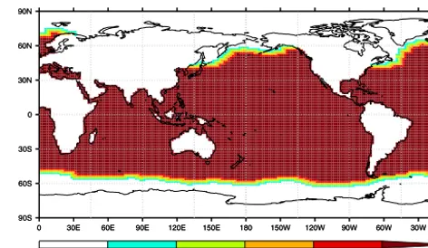
Figure 2. Coupling mask showing the five-grid-point linear blend
between the MetUM-GOML coupling region (α=1; dark red) and
the SST boundary condition outside the coupling region (α=0;
white).
tude horizontal resolution with 85 points in the vertical and a model lid at 85 km.
In MetUM-GOML the MetUM and MC-KPP have been coupled nearly globally as shown in Fig. 2. The latitudinal extent of the MetUM-GOML coupling domain has been de-termined taking into account regions of seasonally varying sea ice because MC-KPP does not include a sea ice model. This was done using the sea ice data set from the Atmo-spheric Model Intercomparison Project (AMIP) component of the Coupled Model Intercomparison Project phase 5 (Tay-lor et al., 2012): coupling was not applied at points which had 30 days year−1of ice for≥3 years in the data set. Fi-nally, the resulting coupling edge was smoothed to create the near-globally coupled MetUM-GOML domain (Fig. 2). Out-side the coupled region, the MetUM is forced by daily cli-matological (1980–2009) SSTs from the Met Office ocean analysis (Smith and Murphey, 2007) and sea ice from the AMIP data set (Taylor et al., 2012), with a five-grid-point linear blend at the boundary.
The depth-varying temperature and salinity corrections were computed from a 10-year, coupled MetUM-GOML in-tegration (K-O-RLX) in which 3-D profiles of salinity and temperature were strongly constrained to the Met Office ocean analysis (Smith and Murphey, 2007) with a 15-day re-laxation timescaleτ. The mean seasonal cycle of tendencies from K-O-RLX are then imposed in free-running MetUM-GOML simulations (Sect. 2.3). Different choices ofτ were tested (e.g. 5, 15, 30, and 90 days) to find a suitable timescale which sufficiently constrained the salinity and temperature profiles without damping subseasonal variability. A 15-day relaxation timescale was chosen because it produced the smallest SST biases in the free-running, coupled simulation. Longer timescales produced larger SST biases since the re-laxation was too weak to counter the SST drift, which arises from the lack of ocean dynamics and biases in atmospheric surface fluxes. With the shorter (5-day) timescale, the atmo-spheric surface fluxes did not adequately adjust to the pres-ence of coupling in the relaxation simulation. This led to a substantial difference between the surface-flux climatologies of the free-running and relaxation simulations, for which the temperature and salinity tendencies could not correct, and hence larger SST biases than the simulation in which the 15-day relaxation was used.
2.3 Experimental setup
All experiments in the present study use the MetUM AGCM at the fixed scientific configuration Global Atmosphere 3.0 (GA3.0; Arribas et al., 2011; Walters et al., 2011). Cou-pled simulations use the ocean mixed-layer, couCou-pled con-figuration MetUM-GOML1, comprising the MetUM GA3.0 coupled to MC-KPP1.0 (as described above). The experi-ments are labelled in the form (experiment type)−(ocean condition), where experiment type describes whether the Me-tUM is coupled to MC-KPP (“K”) or run in atmosphere-only mode (“A”). The ocean condition describes either the data set to which the simulation is constrained, in the case of coupled simulations, or the SST boundary condition used to force the atmosphere-only simulations. The coupled simulations here are constrained to the mean seasonal cycle (1980–2009) of observed (“O”) ocean temperature and salinity from the Met Office ocean analysis (Smith and Murphey, 2007; Fig. 2).
To test this model configuration and investigate the role of well-resolved upper-ocean coupling, three sets of ex-periments have been conducted. K-O describes the free-running MetUM-GOML simulations in which the climato-logical temperature and salinity corrections from the strongly constrained K-O-RLX simulation are applied. Three K-O simulations have been run for 25 years each, initialised from 1 January of year 10, 9 and 8 of the 10-year K-O-RLX simulation, respectively. The coupled integrations are com-pared with two sets of atmosphere-only simulations forced by (a) the daily mean seasonal cycle of SSTs averaged over 60 years of K-O (years 6–25 of each K-O simulation): A-Kcl,
and (b) 31-day smoothed SSTs from the three K-O simula-tions: A-K31. The A-K31 experiment is designed to mimic the AMIP-style setup of forcing with monthly-mean SSTs. A 31-day running mean produces a smoother SST time series than interpolating monthly means to daily values. The initial-isation and run length of the A-Kcl and A-K31 simulations are identical to those of the K-O simulations. The first five years of each simulation have been excluded from the anal-ysis, and the following 20 years (years 6–25) contribute to the results shown here. Therefore, 60 years from each exper-iment have been analysed. The experexper-iments are summarised in Table 1.
In this experimental setup the impact of introducing in-terannual variability in SSTs (A-K31 minus A-Kcl) can be separated from the impact of coupling feedbacks (K-O mi-nus A-K31; Table 2) within a model that, by construction, has a close-to-observed basic state. However, since the K-O SSTs used to force A-K31 have undergone a 31-day smooth-ing, the latter comparison (K-O minus A-K31) includes the effect of sub-31-day SST variability as well as the impact of coupling feedbacks.
2.4 Observational data sets
The evaluation of the mean state (Sect. 3) and tropical and extratropical variability (Sect. 4) in the MetUM sim-ulations is made through comparisons with three observa-tional data sets. Daily instantaneous (00Z), pressure-level specific humidity, zonal wind, temperature and geopotential height data are taken from the European Centre for Medium-range Weather Forecasts Interim reanalysis (ERA-Interim; Dee et al., 2011) for 1990–2009. Rainfall data are taken from the Tropical Rainfall Measuring Mission (TRMM; Kum-merow et al., 1998) 3B42 product, version 6, for 1999– 2011 on a 0.25◦×0.25◦grid. Outgoing longwave radiation (OLR) data are taken from the National Oceanic and Atmo-spheric Administration (NOAA) Advanced Very High Res-olution Radiometer (AVHRR) data set for 1989–2009 on a 2.5◦×2.5◦grid. Where direct comparisons are made be-tween the MetUM and ERA-Interim and TRMM, the obser-vational data have been interpolated to the MetUM grid using an area-weighted interpolation method. Where comparisons have been made with NOAA data, the MetUM simulations have been interpolated to the NOAA grid.
Table 1. Summary of simulations carried out in the current study.
Experiment Coupling Ocean condition Simulations×years
K-O MC-KPP near-global (K) Mean seasonal cycle from observations (O; Smith and Murphey, 2007) 3×25
A-K31 Atmosphere-only (A) 31-day smoothed K-O (K31) 3×25
A-Kcl Atmosphere-only (A) Mean seasonal cycle from K-O (Kcl) 3×25
Table 2. Focus comparisons of experiments in the study and the
impacts revealed by each.
Comparison Impact of
K-O minus A-K31 Coupling feedbacks
A-K31 minus A-Kcl Interannual variability in SST
K-O minus A-Kcl Combined effect
3.1 Zonal-mean vertical structure
Analysing the annual-mean zonal-mean vertical structure of temperature and specific humidity shows that the MetUM is more than 1 g kg−1too dry in the tropical lower-troposphere (not shown), up to 4◦C too warm throughout the stratosphere
and up to 2◦C too cold in much of the troposphere (Fig. 3a)
compared with ERA-Interim reanalysis. These differences are not seasonally dependent, although the tropospheric cool-ing is stronger in the Northern Hemisphere durcool-ing winter and spring.
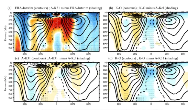
Compared with A-Kcl, K-O warms and dries the tropi-cal lower-troposphere by approximately 0.6 K (Fig. 3b) and 0.4 g kg−1 (not shown), respectively, while the stratosphere in the Southern (Northern) Hemisphere is cooled (warmed) slightly (Fig. 3b). These changes in the zonal-mean vertical structure of temperature and specific humidity are a result of the coupling feedbacks in K-O (Fig. 3d) rather than the intro-duction of interannual variability in SST in the atmosphere-only configuration (A-K31; Fig. 3c). The inclusion of air–sea interactions has the added impact of slightly cooling the trop-ical upper troposphere (Fig. 3d) which suggests that overall convection is slightly shallower in K-O compared with A-K31.
The upper-level subtropical jets in the MetUM are shifted equatorward compared with ERA-Interim (Fig. 4a), partic-ularly in the Northern Hemisphere. This results in a tropical westerly bias at upper-levels compared with ERA-Interim. In K-O, the subtropical jet in the Southern Hemisphere is nar-rowed and the magnitude of the equatorial upper-level west-erly bias is reduced (Fig. 4b). These changes are a conse-quence of the introduction of interannual variability in SST (Fig. 4c) and the air–sea coupling feedbacks (Fig. 4d), re-spectively.
3.2 Precipitation
Compared with TRMM all MetUM simulations exhibit wet annual-mean precipitation biases over the equatorial Indian Ocean (IO) and the South Pacific convergence zone (SPCZ) and dry annual-mean precipitation biases over the Indian subcontinent, Australia and the MC islands (Fig. 5b). This is a long-standing and well-documented bias in the Me-tUM (e.g. Ringer et al., 2006), which was also present in CMIP3 models and not improved in CMIP5 (Sperber et al., 2013). Figure 5c shows the tropical precipitation biases in the fully coupled MetUM-NEMO configuration. While they are of similar magnitude to those in A-K31, they differ in their spatial distribution: in MetUM-NEMO the equato-rial IO bias is focused in the western IO and a dry bias is present in the western Pacific warm pool region (Fig. 5c). These differences are a result of different biases in SST in the MetUM-GOML model compared with MetUM-NEMO (Fig. 1). Compared with the MetUM-NEMO configuration, A-K31 increases precipitation in the central IO and equato-rial Pacific and reduces precipitation in the western IO and off-equatorial regions of the Pacific (Fig. 5d).
Coupling the MetUM to MC-KPP reduces this precipi-tation bias by drying the equatorial IO and SPCZ and in-creasing precipitation over the MC islands; however, little improvement is made to the significant dry biases over con-tinental India. Introducing interannual variability in SST can account for most of the reduction in rainfall over the equa-torial IO (Fig. 5e) but has little impact in the Pacific. Con-versely, the reduction of the wet bias in the SPCZ is a con-sequence of the coupling feedbacks (Fig. 5f). Over the MC region interannual variability in SST and coupling feedbacks have opposite drying and moistening effects respectively.
This precipitation bias in the MetUM is particularly pro-nounced during the Asian summer monsoon season during which it exhibits weaker-than-observed upper-level winds and deficient (excess) precipitation over India (the equato-rial IO; Ringer et al., 2006). During JJA, the wet precipita-tion bias over the central IO in K-O is reduced by more than 5 mm day−1, largely as a result of the interannual variability in SST introduced in A-K31 (Fig. 5g). Little improvement is made in K-O to the lack of monsoonal precipitation over the Indian subcontinent (Fig. 5g, h).
pat-Zonal-mean T ERA-Interim (contours) and [A-K31 - ERA-Interim] (shading)
-6 -2 -1.4 -1.0 -0.6 -0.2 0.4 0.8 1.2 1.6 4 (K)
annual 60S 30S 0 30N 60N
900 800 700 600 500 400 300 200 100 10 200 210 220 220 220 220 220 220 230 230 230 230 240 240 240 240 250 250 250 250 260 260 260 260 270 270 280 280 290
Zonal-mean T A-Kcl (contours) and [K-O - A-Kcl] (shading)
-6 -2 -1.4 -1.0 -0.6 -0.2 0.4 0.8 1.2 1.6 4 (K)
annual 60S 30S 0 30N 60N
900 800 700 600 500 400 300 200 100 10 200 210 220 220 220 220 220 220 230 230 230 230 240 240 240 240 250 250 250 250 260 260 260 260 270 270 280 280 290
Zonal-mean T A-K31 (contours) and [K-O - A-K31] (shading)
-6 -2 -1.4 -1.0 -0.6 -0.2 0.4 0.8 1.2 1.6 4 (K)
annual 60S 30S 0 30N 60N
900 800 700 600 500 400 300 200 100 10 200 210 220 220 220 220 220 220 230 230 230 230 240 240 240 240 250 250 250 250 260 260 260 260 270 270 280 280 290 Zonal-mean T A-Kcl (contours) and [A-K31 - A-Kcl] (shading)
-6 -2 -1.4 -1.0 -0.6 -0.2 0.4 0.8 1.2 1.6 4 (K)
annual 60S 30S 0 30N 60N
900 800 700 600 500 400 300 200 100 10 200 210 220 220 220 220 220 220 230 230 230 230 240 240 240 240 250 250 250 250 260 260 260 260 270 270 280 280 290
Zonal-mean T A-Kcl (contours) and [K-O - A-Kcl] (shading)
-6 -2 -1.4 -1.0 -0.6 -0.2 0.4 0.8 1.2 1.6 4
(K)
annual 60S 30S 0 30N 60N
900 800 700 600 500 400 300 200 100 10 200 210 220 220 220 220 220 220 230 230 230 230 240 240 240 240 250 250 250 250 260 260 260 260 270 270 280 280 290 (a) ERA-Interim (contours) ; A-K31 minus ERA-Interim (shading)
(d) K-O (contours) ; K-O minus A-K31 (shading) (c) A-K31 (contours) ; A-K31 minus A-Kcl (shading)
(b) K-O (contours) ; K-O minus A-Kcl (shading)
P re ss ure (hP a) P re ss ure (hP a)
Figure 3. (a) Annual-mean zonal-mean temperature from the ERA-Interim (contours) and bias of A-K31 compared with the ERA-Interim
(shading). Impact of interannual SST variability (c; A-K31 minus A-Kcl), coupling (d; K-O minus A-K31) and both SST variability and coupling (b; K-O minus A-Kcl) on the vertical structure of zonal-mean temperature. Stippling indicates where differences are significant at the 95 % level.
Zonal-mean u A-Kcl (contours) and [K-O - A-Kcl] (shading)
-6 -2 -1.4 -1.0 -0.6 -0.2 0.1 0.4 0.8 1.2 1.6 4
(ms-1 )
annual 60S 30S 0 30N 60N
900 800 700 600 500 400 300 200 100
10 -10 -15
-5 -2 -2 -2 -2 2 2 2 2 2 2 2 5 5 5 5 5 5 10 10 10 10 15 15 15 15 20 20 25 25 25 30 30 35
Zonal-mean u A-K31 (contours) and [K-O - A-K31] (shading)
-6 -2 -1.4 -1.0 -0.6 -0.2 0.1 0.4 0.8 1.2 1.6 4
(ms-1 )
annual 60S 30S 0 30N 60N
900 800 700 600 500 400 300 200 100
10 -10 -15
-5 -2 -2 -2 -2 2 2 2 2 2 2 2 5 5 5 5 5 5 10 10 10 10 15 15 15 15 20 20 25 25 25 30 30 35
Zonal-mean u ERA-Interim (contours) and [A-K31 - ERA-Interim] (shading)
-6 -2 -1.4 -1.0 -0.6 -0.2 0.1 0.4 0.8 1.2 1.6 4 (ms-1
)
annual 60S 30S 0 30N 60N 900 800 700 600 500 400 300 200 100
10 -10 -15 -15 -5 -2 -2 -2 -2 2 2 2 2 2 2 5 5 5 5 5 5 10 10 10 10 15 15 15 15 20 20 25 25 25 30 30
Zonal-mean u A-Kcl (contours) and [A-K31 - A-Kcl] (shading)
-6 -2 -1.4 -1.0 -0.6 -0.2 0.1 0.4 0.8 1.2 1.6 4
(ms-1 )
annual 60S 30S 0 30N 60N
900 800 700 600 500 400 300 200 100
10 -10 -15 -15
-5 -2 -2 -2 -2 2 2 2 2 2 2 5 5 5 5 5 5 10 10 10 10 15 15 15 15 20 20 25 25 25 30 30
(a) ERA-Interim (contours) ; A-K31 minus ERA-Interim (shading)
(d) K-O (contours) ; K-O minus A-K31 (shading) (c) A-K31 (contours) ; A-K31 minus A-Kcl (shading)
(b) K-O (contours) ; K-O minus A-Kcl (shading)
P re ss ure (hP a) P re ss ure (hP a)
Zonal-mean u A-Kcl (contours) and [A-K31 - A-Kcl] (shading)
-6 -2 -1.4 -1.0 -0.6 -0.2 0.1 0.4 0.8 1.2 1.6 4
(ms-1)
annual 60S 30S 0 30N 60N
900 800 700 600 500 400 300 200 100
10 -10 -15 -15
-5 -2 -2 -2 -2 2 2 2 2 2 2 5 5 5 5 5 5 10 10 10 10 15 15 15 15 20 20 25 25 25 30 30
Figure 4. As in Fig. 3, but for the annual-mean zonal-mean zonal wind.
terns which, by constraining the K-O ocean temperature and salinity, is close to observations. This allows changes in the variability (Sect. 4) within this modelling framework to be attributed to the impact of introducing interannual variability in SST (A-K31 minus A-Kcl) or having air–sea interactions (K-O minus A-K31), rather than to changes in the basic state of the model.
4 Impact of coupling on variability
Teleconnections between the tropics and extratropics suggest that remote and local air–sea interactions are important to the representation of variability on subseasonal timescales
(Sect. 1.1.3). Aspects of both tropical (Sect. 4.1) and extrat-ropical (Sect. 4.2) variability will be examined in the current simulations.
4.1 Tropical variability
Figure 5. (a) Annual-mean precipitation from A-K31. (b and c) show the annual-mean bias of A-K31 and MetUM-NEMO against TRMM
satellite observations. (d) Change of annual-mean precipitation between A-K31 and MetUM-NEMO. Impact of introducing interannual variability in SST (e, g; A-K31 minus A-Kcl) and having air–sea interactions (f, h; K-O minus A-K31) on annual-mean and JJA (June-July-August) precipitation, respectively. Differences are only shown where they are significant at the 95 % level.
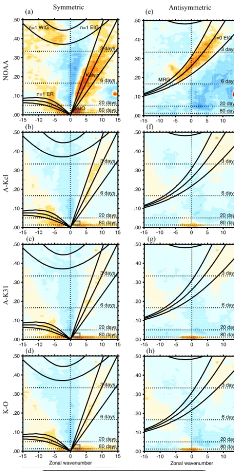
4.1.1 Convectively coupled equatorial waves
A substantial proportion of large-scale organised tropical convection is associated with equatorial waves. Therefore, it is important to examine how these wave modes are rep-resented in these simulations. The organisation of tropical convection by equatorial waves is examined by comput-ing the space–time power spectra of anomalous, equatori-ally averaged (15◦N–15◦S) OLR, as in Wheeler and Ki-ladis (1999). After computing tropical OLR anomalies from the seasonal cycle, the zonal wave number-frequency power spectra are separated into symmetric and antisymmetric com-ponents and the red background spectrum removed. This results in the emergence of preferred space and timescales for organised tropical convection. In NOAA satellite obser-vations these preferred scales are consistent with theoreti-cal equatorial waves, highlighted by the dispersion curves at varying equivalent depths (solid lines). For example, in the observed symmetric spectrum, eastward-propagating Kelvin and westward-propagating equatorial Rossby (ER) waves emerge, as well as a signature of the eastward-propagating
intraseasonal MJO at zonal wave numbers 1–3 (Fig. 6a). In the antisymmetric component the observations exhibit power associated with mixed Rossby-gravity (MRG) and eastward-propagating inertio-gravity (EIG) waves (Fig. 6e).
in-Symmetric/Background power in olr for NOAA 80 days 20 days 6 days 3 days n=1 ER Kelvin MJO
n=1 WIG n=1 EIG
-15 -10 -5 0 5 10 15
Zonal wavenumber .00 .10 .20 .30 .40 .50
0.30.40.50.60.70.80.9 1 1.11.21.41.7 2 2.42.8 LOG10 [Power:15S-15N]
Anti-symmetric/Background power in olr for K-O
80 days 20 days 6 days 3 days
-15 -10 -5 0 5 10 15
Zonal wavenumber .00 .10 .20 .30 .40 .50
0.30.40.50.60.70.80.9 1 1.11.21.41.7 2 2.42.8 LOG10 [Power:15S-15N] Symmetric/Background power in olr for K-O
80 days 20 days 6 days 3 days
-15 -10 -5 0 5 10 15
Zonal wavenumber .00 .10 .20 .30 .40 .50
0.30.40.50.60.70.80.9 1 1.11.21.41.7 2 2.42.8 LOG10 [Power:15S-15N]
Anti-symmetric/Background power in olr for A-Kcl
80 days 20 days 6 days 3 days
-15 -10 -5 0 5 10 15
Zonal wavenumber .00 .10 .20 .30 .40 .50
0.30.40.50.60.70.80.9 1 1.11.21.41.7 2 2.42.8 LOG10 [Power:15S-15N] Symmetric/Background power in olr for A-Kcl
80 days 20 days 6 days 3 days
-15 -10 -5 0 5 10 15
Zonal wavenumber .00 .10 .20 .30 .40 .50
0.30.40.50.60.70.80.9 1 1.11.21.41.7 2 2.42.8 LOG10 [Power:15S-15N]
Anti-symmetric/Background power in olr for A-K31
80 days 20 days 6 days 3 days
-15 -10 -5 0 5 10 15
Zonal wavenumber .00 .10 .20 .30 .40 .50
0.30.40.50.60.70.80.9 1 1.11.21.41.7 2 2.42.8 LOG10 [Power:15S-15N] Symmetric/Background power in olr for A-K31
80 days 20 days 6 days 3 days
-15 -10 -5 0 5 10 15
Zonal wavenumber .00 .10 .20 .30 .40 .50
0.30.40.50.60.70.80.9 1 1.11.21.41.7 2 2.42.8 LOG10 [Power:15S-15N]
Anti-symmetric/Background power in olr for NOAA
80 days 20 days 6 days 3 days MRG n=0 EIG
-15 -10 -5 0 5 10 15
Zonal wavenumber 0.00 0.10 0.20 0.30 0.40 0.50
0.3 0.4 0.5 0.6 0.7 0.8 0.9 1 1.1 1.2 1.4 1.7 2 2.4 2.8
LOG10 [Power:15S-15N] (a) (b) (c) (d) (e) (f) (g) (h) NOAA A -K cl A -K 31 K -O Symmetric Antisymmetric
Anti-symmetric/Background power in olr for NOAA
80 days 20 days 6 days 3 days MRG n=0 EIG
-15 -10 -5 0 5 10 15
Zonal wavenumber .00 .10 .20 .30 .40 .50
0.30.40.50.60.70.80.9 1 1.11.21.41.7 2 2.42.8 LOG10 [Power:15S-15N]
Figure 6. Zonal wave number-frequency power spectra of
anoma-lous OLR for symmetric (a–d) and antisymmetric (e–h) compo-nents divided by the background power for NOAA satellite obser-vations (a, e), A-Kcl (b, f), A-K31 (c, g) and K-O (d, h). Solid lines represent dispersion curves at equivalent depths of 12, 25 and 50 m. Theoretical modes highlighted in observations: ER, Kelvin, MJO, MRG, and eastward and westward inertio-gravity (EIG, WIG). The grey box indicates the MJO spectral region of 30–80 days and wave numbers 1–3.
crease the magnitude of MJO power and slightly broaden that power over a wider frequency range. As a complex, multi-scale phenomenon the MJO, and teleconnection patterns as-sociated with it, acts as a rigorous test for GCMs and hence its representation in these simulations warrants further inves-tigation (Sect. 4.1.2).
4.1.2 The Madden–Julian Oscillation
Intraseasonal variability in the tropical atmosphere–ocean system is dominated by the MJO (e.g. Madden and Ju-lian, 1972; Zhang, 2005). The active phase of the MJO can be characterised as a planetary-scale envelope of organised deep convection which propagates eastward from the Indian Ocean into the western Pacific. Ahead and behind the deep convective centre are areas of suppressed convection. The ac-tive and suppressed phases of the MJO are connected by a strong overturning circulation in the zonal wind. Significant effort has gone into defining indices and diagnostics which fully describe the representation of the MJO in observations and model simulations (e.g. Wheeler and Hendon, 2004; Kim et al., 2009).
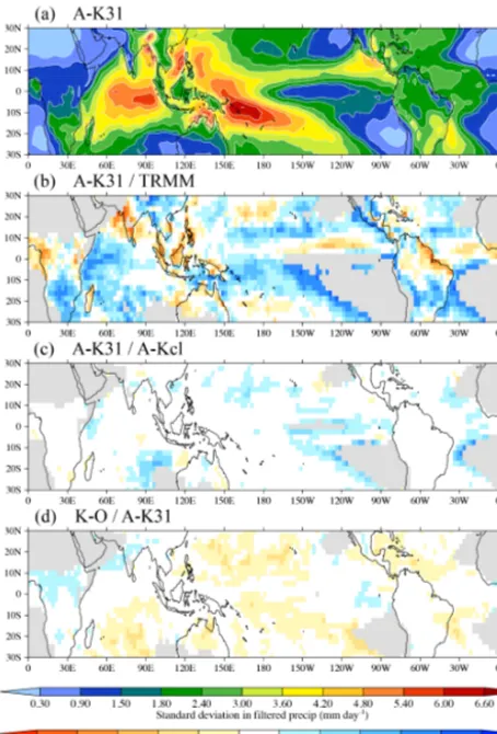
One such diagnostic is to extract variability associated with the MJO by bandpass filtering fields, such as precipita-tion, to MJO timescales (e.g. 20–80 days). The standard devi-ation in 20–80-day filtered precipitdevi-ation from A-K31 shows maxima in variability located over the equatorial Indo-Pacific (Fig. 7a). Comparison with TRMM satellite data shows that the A-K31 overestimates intraseasonal variability in precip-itation over the equatorial IO, SPCZ, southern Africa and north of Australia (Fig. 7b); this is consistent with the over-estimation of the mean precipitation in these regions (Fig. 5). Conversely, intraseasonal variability in precipitation is un-derestimated in A-K31 over the Gulf of Guinea and the In-dian subcontinent. Introducing interannual variability in SST has little impact on these biases in the variability of intrasea-sonal precipitation (Fig. 7b). Including air–sea interactions in K-O generally reduces intraseasonal variability in precipita-tion over the equatorial oceans and increases variability over central Africa and India (Fig. 7d). These changes in variabil-ity result in a better representation of intraseasonal precipita-tion in K-O; this is also consistent with the mean-state change in precipitation shown in Fig. 5.
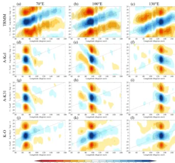
To assess the zonal propagation of the MJO in the MetUM, lag regressions of latitude-averaged (15◦N–15◦S), 20–80-day bandpass filtered precipitation are computed using three base points: in the central Indian Ocean (70◦E), the western
edge of the maritime continent (100◦E) and the western
Pa-cific (130◦E). This is a further diagnostic recommended by the CLIVAR MJO Task Force (Kim et al., 2009), which has previously been applied to MJO-filtered OLR to investigate the role of local air–sea interactions in the MetUM GA3.0 (Klingaman and Woolnough, 2014).
Figure 7. Standard deviation in 20–80-day filtered precipitation
from (a) A-K31. Ratio of standard deviations from A-K31 and TRMM (b), A-K31 and A-Kcl (c; impact of SST variability) and K-O and A-K31 (d; impact of coupling). In (b–d), regions with a standard deviation of filtered precipitation below 1 mm day−1have been excluded from the ratio calculation and masked grey.
along the dashed line which represents the approximate ob-served phase speed of the MJO. In A-Kcl, subseasonal vari-ability in precipitation is either stationary or propagates to the west (Fig. 8d–f). Introducing interannual variability in SST in A-K31 reduces the extent of westward propagation of sub-seasonal precipitation, especially over the maritime continent (Fig. 8h compared with Fig. 8e). The eastward propagation of subseasonal variability in precipitation is only achieved with the inclusion of air–sea interactions in K-O (Fig. 8j–l). Al-though the magnitude of the anomalies remain weaker than observed, K-O is able to produce anomalies which propagate at the correct phase speed (compared with dashed line). The transition from westward-propagating (in A-Kcl and A-K31) to eastward-propagating (in K-O) intraseasonal precipitation anomalies is especially striking over the maritime continent (base point 100◦E; Fig. 8e, h, k), a region in which mod-els typically struggle to maintain the MJO signal (e.g. Vitart and Molteni, 2009). The impact of air–sea interactions on
the eastward propagation of the MJO here within the near-globally coupled MetUM-GOML is consistent with a similar MetUM mixed-layer ocean coupled simulation with coupling only in the Indo-Pacific (Klingaman and Woolnough, 2014). It is clear that air–sea interactions play an important role in the representation of tropical subseasonal variability. Specifi-cally, K-O has shown a distinct improvement in the represen-tation of tropical variability associated with the MJO. How-ever, deficiencies remain in the simulation of MJO activity in K-O. While air–sea interactions have improved the prop-agation of the MJO in the MetUM (Fig. 8), the amplitude of MJO activity remains significantly weaker than in observa-tions (Fig. 6). Existing studies suggest that MJO-related trop-ical heating anomalies can excite wave trains which propa-gate polewards and modulate aspects of variability in the ex-tratropics (e.g. Cassou, 2008). If the improvements in MJO activity are large enough and the MetUM is able to accurately represent the circulation response to the MJO then, through this tropical–extratropical teleconnection, changes may also be expected in the representation of the extratropical variabil-ity in K-O. This is examined in Sect. 4.2 through investiga-tion of the Northern Hemisphere storm tracks and blocking frequency.
4.2 Extratropical variability
Analysis of the role of air–sea interactions on the represen-tation of extratropical variability is focused on the Northern Hemisphere storm tracks and blocking.
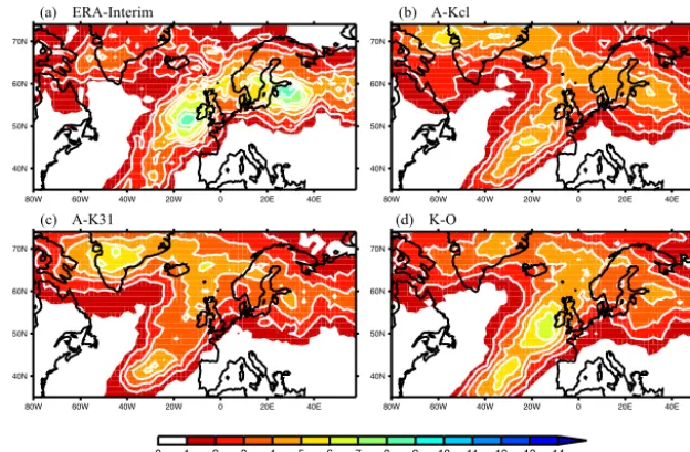
4.2.1 Northern Hemisphere storm tracks
Daily variability in the Northern Hemisphere midlatitudes is largely controlled by the Atlantic and Pacific storm tracks. Cyclones originating in the western Atlantic and Pacific oceans move east along a preferred path or storm track, bringing significant precipitation and strong winds to Europe and North America. Because variations in these storm tracks modulate the continental climate of the Northern Hemi-sphere, their representation in GCMs is important.
Previous analyses of storm track activity in GCMs fall into two broad categories: feature tracking of weather sys-tems (e.g. Hoskins and Hodges, 2002) and 2–6-day band-pass filtering (e.g. 500 hPa geopotential height; Blackmon, 1979). The application of these techniques within coupled and atmosphere-only configurations of the MetUM yield broadly consistent results (Martin et al., 2004). Here, the lat-ter is applied: 24-hourly instantaneous geopotential heights at 500 hPa are bandpass filtered between 2 and 6 days. This method isolates the high-frequency eddy activity in the mid-troposphere, which, by identifying the passage of synoptic weather systems, is a reliable indication of the location of the storm tracks.
bandpass-Figure 8. Lag regressions of latitude-averaged (15◦N–15◦S), 20–80-day bandpass-filtered precipitation against base points in the central Indian Ocean (70◦E; a, d, g, j), maritime continent (100◦E; b, e, h, k) and western Pacific (130◦E; c, f, i, l). Positive and negative days represent lags and leads, respectively. Approximate observed propagation speeds are shown by the dashed lines. Stippling indicates where the lag regressions are significant at the 95 % level.
filtered geopotential heights at 500 hPa from A-K31 in the Northern Hemisphere. There are two clear areas of activ-ity over the midlatitude Pacific and Atlantic ocean basins, with the eddy activity maxima, where cyclogenesis is most common, over the west of the respective basins. The over-all location of the storm tracks in the MetUM is similar to ERA-Interim, with eddy maxima occurring in the right place. There is a slight equatorward bias in the storm tracks over the ocean compared with ERA-Interim (Fig. 9b, c) which is consistent with the equatorward shift of the Northern Hemi-sphere subtropical jet seen in Fig. 4a. In the MetUM there is generally not enough eddy activity; the Atlantic storm track does not extend far enough into Europe, and the Pacific track is too weak (Fig. 9b, c). Introducing interannual variability in SST slightly broadens the area of strong eddy activity into the northern Pacific but has little impact on the extension of the Atlantic track into Europe (Fig. 9d). Introducing air–sea interactions in K-O has little impact on the representation of the Pacific and Atlantic storm tracks compared with A-K31 (Fig. 9e). The limited impact on the Northern Hemisphere storm tracks in K-O suggests that the improvements in trop-ical intraseasonal variability may not be sufficiently large to
influence extratropical variability, at least by this measure. It may also be that horizontal resolution plays a role; the simu-lations shown here may be too coarse to sufficiently capture the extratropical variability, no matter how well the tropical intraseasonal variability is represented.
4.2.2 Northern Hemisphere blocking
lat-Figure 9. Standard deviation in wintertime (DJF) 2–6-day bandpass-filtered 500 hPa geopotential height over the Northern Hemisphere from
A-K31 (a). Ratio of standard deviations from A-K31 and ERA-Interim (b), K-O and ERA-Interim (c), A-K31 and A-Kcl (d; impact of SST variability), K-O and A-K31 (e; impact of coupling) and K-O and A-Kcl (f; impact of both). Changes in variance are only shown where they are significant at the 95 % level.
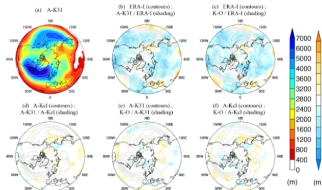
itude and if both these criteria hold for at least 5 consec-utive days. This analysis yields a daily binary 2-D map of persistent quasi-stationary blocked grid points. In the Euro-Atlantic sector atmospheric blocking is most prominent dur-ing the winter and sprdur-ing seasons; the MAM (March-April-May) blocking frequencies for ERA-Interim and the MetUM simulations are shown in Fig. 10.
In the ERA-Interim, there are two maxima in MAM block-ing frequency: off the south-west coast of Ireland and over the Baltic region (Fig. 10a). The MetUM is broadly able to represent the spatial pattern of blocking in DJF (not shown) and MAM (Fig. 10) but underestimates the fre-quency of blocking events. Specifically, A-Kcl does indi-cate blocking frequency maxima in the correct locations compared with ERA-Interim, although they are consider-ably weaker than observed. Furthermore, A-Kcl exhibits too much blocking activity over Greenland and Baffin Bay (Fig. 10b). Interannual variability in SST does not improve this bias but further increases blocking activity over Green-land and weakens blocking activity in the observed max-ima regions (Fig. 10c). Including near-global air–sea inter-actions increases the blocking frequency off the south-west coast of Ireland and decreases blocking over Greenland, re-sulting in a closer-to-observed blocking frequency pattern (Fig. 10d). Interestingly, K-O is not coupled in the seas sur-rounding Greenland, suggesting the change of blocking fre-quency there is an impact of non-local coupling. Blocking frequency over the Baltic region remains underestimated in all MetUM simulations. During DJF the MetUM underesti-mates blocking frequency over the UK and Scandinavia com-pared with the ERA-Interim; this remains the case even with the introduction of interannual variability in SST and cou-pling feedbacks (not shown).
This initial analysis suggests that introducing air–sea in-teractions in K-O changes the distribution and frequency of blocking events in the Northern Hemisphere. With the im-proved representation of tropical variability associated with the MJO in K-O (Sect. 4.1.2), and the known link between the MJO and extratropical variability (e.g. Cassou, 2008), this is an appropriate modelling framework to investigate the relative roles of local and remote coupling on these modes of variability and the teleconnections linking them (see Sect. 5 for further discussion).
5 Discussion and conclusions
A new coupled modelling framework (MetUM-GOML) has been described in which an AGCM is coupled to a high-resolution, vertically resolved mixed-layer ocean. This is the first coupled system that is capable of providing well-resolved air–sea interactions at limited additional computa-tional expense, enabling high-resolution, climate length inte-grations.
80W 60W 40W 20W 0 20E 40E 40N
50N 60N 70N
0 1 2 3 4 5 6 7 8 9 10 11 12 13 14
% of blocked days
A-Kcl Euro-Atlantic MAM blocking frequency
80W 60W 40W 20W 0 20E 40E
40N 50N 60N 70N
0 1 2 3 4 5 6 7 8 9 10 11 12 13 14
% of blocked days
ERA-INT Euro-Atlantic MAM blocking frequency
80W 60W 40W 20W 0 20E 40E
40N 50N 60N 70N
0 1 2 3 4 5 6 7 8 9 10 11 12 13 14
% of blocked days
K-O Euro-Atlantic MAM blocking frequency
80W 60W 40W 20W 0 20E 40E
40N 50N 60N 70N
0 1 2 3 4 5 6 7 8 9 10 11 12 13 14
% of blocked days
A-K31 Euro-Atlantic MAM blocking frequency
80W 60W 40W 20W 0 20E 40E
40N 50N 60N 70N
0 1 2 3 4 5 6 7 8 9 10 11 12 13 14
% of blocked days
ERA-INT Euro-Atlantic MAM blocking frequency
(a) ERA-Interim (b) A-Kcl
(c) A-K31 (d) K-O
Figure 10. Euro-Atlantic springtime (MAM) blocking frequency climatology using the absolute geopotential height index calculated from
the 500 hPa geopotential heights after Tibaldi and Molteni (1990) and Scherrer et al. (2006).
MetUM-GOML simulations were performed (K-O) as well as MetUM atmosphere-only simulations forced by 31-day smoothed SSTs (A-K31) or the mean seasonal cycle of SSTs (A-Kcl) from K-O (Table 1). This allowed the impact of introducing interannual variability in SST (A-K31 minus A-Kcl) to be separated from the impact of coupling feed-backs (K-O minus A-K31). It should be noted that since the K-O SSTs used to force A-K31 have undergone a 31-day smoothing, the latter comparison (K-O minus A-K31) includes the effect of increased, higher frequency SST vari-ability as well as coupling feedbacks.
The performance of these simulations has been assessed by comparing the representation of their mean state and analysing their ability to reproduce several aspects of tropical and extratropical variability. Compared with ERA-Interim reanalysis, the MetUM is shown to be too warm in the strato-sphere, too cool and dry in the tropical mid- and lower tro-posphere and have an equatorward shift in the subtropical jets. Introducing variability in SST is shown to slightly nar-row the Southern Hemisphere subtropical jet, while coupling is shown to warm and dry above the boundary layer, cool the upper troposphere and reduce the upper-level equatorial westerly bias. However, all of these tropospheric mean-state changes are small in magnitude (Figs. 3, 4). Larger differ-ences are seen in the representation of tropical precipitation. SST variability reduces precipitation over the equatorial In-dian Ocean and maritime continent; coupling reduces (in-creases) precipitation over the SPCZ and equatorial Indian Ocean (maritime continent). These changes result in a reduc-tion in the long standing equatorial Indian Ocean dry bias (Ringer et al., 2006; Sperber et al., 2013), but have little im-pact on the lack of monsoonal precipitation over the Indian subcontinent in the MetUM (Fig. 5).
Consistent with the mean-state changes described above, coupling improves the distribution and variability of intrasea-sonal convection in the tropics (Fig. 7). A detailed exami-nation of convectively coupled equatorial wave modes indi-cates that all the MetUM simulations underestimate or, in some cases, fail to capture the variability corresponding to observed wave modes. Coupling is shown to concentrate the eastward power associated with the MJO and reduce spurious low-frequency westward power (Fig. 6). In fact, the propaga-tion of the MJO is significantly improved in K-O; coupling feedbacks transform the MJO signal from stationary or west-ward propagating precipitation anomalies in A-K31 to a clear eastward propagating signal. This MJO signal, however, re-mains weaker than in observations (Fig. 8).
The influence of air–sea coupling has also been examined in the extratropics. In the MetUM, the Northern Hemisphere Pacific storm track is too weak and the Atlantic track does not extend far enough into Europe. Introducing interannual variability in SST broadens the area of strong eddy activ-ity in the Pacific but coupling has little impact on the storm tracks in either basin (Fig. 9). However, coupling feedbacks do appear to slightly improve the frequency of atmospheric blocking over the Euro-Atlantic sector, although this remains lower than observed (Fig. 10).
In terms of the diagnostics considered here, MetUM-GOML has generally been shown to slightly improve the rep-resentation of tropical and extratropical variability compared with its atmosphere-only counterpart. With a more accurate representation of variability, this framework could be used as a test bed for investigating how global weather and climate extremes may change in a warming world.
pro-vides a new and exciting research tool for process-based studies of air–sea interactions. The limited computational cost enables coupling to be applied at higher GCM horizon-tal resolution; the current framework has also been imple-mented with the MetUM at horizontal resolutions of ∼60 and ∼25 km (the simulations described here are∼135 km resolution). Results from these integrations will form the ba-sis of future studies. Furthermore, the technical advantages described in Sect. 1.3 present many opportunities for further sensitivity studies. The controllability of this framework, for example, could be used to constrain the ocean to a particu-lar mode of variability from interannual (ENSO) and decadal (PDO) to multi-decadal (AMO) timescales to investigate the role coupling plays in the teleconnection patterns associated with that pattern of oceanic variability. Alternatively, by con-straining MC-KPP to a model ocean climatology, MetUM-GOML could be used to investigate the role of regional SST biases. Within coupled simulations using a full dynamical ocean, changes in the coupled mean state are often compen-sated by large biases in the coupled system. With this frame-work, the impact of particular regional SST biases could be investigated remaining within a framework that represents air–sea interactions. Furthermore, the adaptable nature of the framework could be exploited to selectively couple (or un-couple) in local regions of interest to investigate the relative role of local and remote air–sea interactions on various at-mospheric phenomena. As a research tool, this new coupled modelling framework will be applied in many future contexts and studies.
Code availability
The source code for MC-KPP version 1.0 is available in the subversion repository at https://puma.nerc.ac.uk/ svn/KPP_ocean_svn/KPP_ocean/tags/MC-KPP_vn1.0. Fur-ther description and information about the MC-KPP model is available at https://puma.nerc.ac.uk/trac/KPP_ ocean and further information regarding MetUM-GOML is available at https://puma.nerc.ac.uk/trac/KPP_ocean/wiki/ MetUM-GOML.
Acknowledgements. The authors were funded by the National Centre for Atmospheric Science (NCAS), a collaborative centre of the Natural Environment Research Council (NERC), under contract R8/H12/83/001. The authors acknowledge productive discussions with Rowan Sutton and Len Shaffrey within NCAS at the University of Reading. This work made use of the facili-ties of HECToR, the UK national high-performance computing service, which is provided by UoE HPCx Ltd at the University of Edinburgh, Cray Inc. and NAG Ltd, and funded by the Office of Science and Technology through EPSRC’s High End Computing Programme.
Edited by: O. Marti
References
Alexander, M. A., Scott, J. D., and Deser, C.: Processes that influ-ence sea surface temperature and ocean mixed layer depth vari-ability in a coupled model, J. Geophys. Res, 105, 16823–16842, 2000.
Arribas, A., Glover, M., Maidens, A., Peterson, K., Gordon, M., MacLachlan, C. D., Fereday, R. G., Camp, J., Scaife, A. A., Xavier, P., Coleman, A., and Cusack, S.: The GloSea4 ensemble prediction system for seasonal forecasting, Mon. Weather Rev., 139, 1891–1910, 2011.
Benedict, J. J. and Randall, D. A.: Impacts of Idealized Air-Sea coupling on Madden-Julian Oscillation sctructure in the Super-parameterized CAM, J. Atmos. Sci., 68, 1990–2008, 2011. Bernie, A. J., Guilyardi, E., Madec, G., Slingo, J. M., Woolnough,
S. J., and Cole, J.: Impact of resolving the diurnal cycle in an ocean-atmosphere GCM. Part 2: A diurnally coupled CGCM, Clim. Dynam., 31, 909–925, 2008.
Bhatt, U. S., Alexander, M. A., Battisti, D. S., Houghton, D. D., and Keller, L. M.: Atmosphere-Ocean Interaction in the North Atlantic: Near-Surface Climate Variability, J. Climate, 11, 1615– 1632, 1998.
Blackmon, M. L.: A Climatological Spectral Study of the 500 mb Geopotential Height of the Northern Hemisphere, J. Atmos. Sci., 33, 1607–1623, 1979.
Cassou, C.: Intraseasonal interaction between the Madden-Julian Oscillation and the North Atlantic Oscillation, Nature, 455, 523– 527, 2008.
Cassou, C., Terray, L., and Phillips, A. S.: Tropical Atlantic Influ-ence on European Heat Waves, J. Climate, 18, 2805–2811, 2005. Cassou, C., Deser, C., and Alexander, M. A.: Investigating the Im-pact of Reemerging Sea Surface Temperature Anomlaies on the Winter Atmospheric Circulation over the North Atlantic, J. Cli-mate, 20, 3510–3526, 2007.
Crueger, T., Stevens, B., and Brokopf, R.: The Madden-Julian Os-cillation in ECHAM6 and the introduction of an objective MJO Index, J. Climate, 26, 3241–3257, 2013.
Dee, D. P., Uppala, S. M., Simmons, A. J., Berrisford, P., Poli, P., Kobayashi, S., Andrae, U., Balmaseda, M. A., Balsamo, G., Bauer, P., Bechtold, P., Beljaars, A. C. M., van de Berg, L., Bid-lot, J., Bormann, N., Delsol, C., Dragani, R., Fuentes, M., Geer, A. J., Haimberger, L., Healy, S. B., Hersbach, H., Holm, E. V., Isaksen, L., Kallberg, P., Kohler, M., Matricardi, M., McNally, A. P., Monge-Sanz, B. M., Morcrette, J.-J., Park, B.-K., Peuby, C., de Rosnay, P., Tavolato, C., Thepaut, J.-N., and Vitart, F.: The ERA-Interim reanalysis: configuration and performance of the data assimilation system, Q. J. Roy. Meteorol. Soc., 137, 553– 597, 2011.
DeMott, C. A., Stan, C., Randall, D. A., and Branson, M. D.: In-traseasonal Variability in Coupled GCMs: The Roles of Ocean Feedbacks and Model Physics, J. Climate, 27, 4970–4995, 2014. Doblas-Reyes, F., Casado, M. J., and Pastor, M. A.: Sensitiv-ity of the Northern Hemisphere blocking frequency to the detection index, J. Geophys. Res., 107, ACL6.1–ACL.6.22, doi:10.1029/2000JD000290, 2002.
Feudale, L. and Shukla, J.: Influence of sea surface temperature on the European heat wave of 2003 summer. Part I: an observational study, Clim. Dynam., 36, 1691–1703, 2011.
Sur-face Temperature in the Indian Ocean, J. Atmos. Sci., 60, 1733– 1753, 2003.
Giannini, A., Saravanan, R., and Chang, P.: Oceanic Forcing of Sa-hel Rainfall on Interannual to Interdecadal Time Scales, Science, 302, 1027–1030, 2003.
Guemas, V., Salas-Mèlia, D., Kageyama, M., Giordani, H., and Voldoire, A.: Impact of the ocean diurnal cycle on the North Atlantic mean sea surface temperatures in a regionally coupled model, Dynam. Atmos. Oceans., 60, 28–45, 2013.
Ham, Y.-G. and Kug, J.-S.: Impact of diurnal atmosphere-ocean coupling on tropical climate simulations using a coupled GCM, Clim. Dynam., 34, 905–917, 2010.
Hendon, H. H. and Liebmann, B.: The Intraseasonal (30–50 day) Oscillation of the Australian Summer Monsoon, J. Atmos. Sci., 47, 2909–2923, 1990.
Hendon, H. H., Lim, E.-P., and Luo, G.: The Role of Air-Sea Inter-action for Prediction of Australian Summer Monsoon Rainfall, J. Climate, 25, 1278–1290, 2012.
Hoskins, B. J. and Hodges, K. I.: New Perspectives on the North-ern Hemisphere Winter Storm Tracks, J. Atmos. Sci., 59, 1041– 1061, 2002.
Inness, P. M., Slingo, J. M., Guilyardi, E., and Cole, J.: Simulation of the Madden-Julian Oscillation in a Coupled General Circula-tion Model: Part II: The Role of the Basic State, J. Climate, 16, 365–382, 2003.
Jullien, S., Marchesiello, P., Menkes, C. E., Lefévre, J., Jourdain, N. C., Samson, G., and Lengaigne, M.: Ocean feedback to trop-ical cyclones: climatology and processes, Clim. Dynam., 43, 2831–2854, 2014.
Kim, D., Sperber, K., Stern, W., Waliser, D., Kang, I.-S., Maloney, E. D., Wang, W., Weickmann, K. J., Benedict, M. K., Lee, M.-I., Neale, R., Suarez, M., Thayer-Calder, K., and Zhang, G.: Ap-plication of MJO Simulation Diagnostics to Climate Models, J. Climate, 22, 6413–6436, 2009.
Klingaman, N. P. and Woolnough, S. J.: The Role of air–sea cou-pling in the simulation of the Madden-Julian oscillation in the Hadley Centre model, Q. J. Roy. Meteorol. Soc., 140, 2272– 2286, doi:10.1002/qj.2295, 2014.
Klingaman, N. P., Woolnough, S. J., Weller, H., and Slingo, J. M.: The Impact of Finer-Resolution Air-Sea Coupling on the In-traseasonal Oscillation of the Indian Monsoon, J. Climate, 24, 2451–2468, 2011.
Kummerow, C., Barnes, W., Kozu, T., Shiue, J., and Simpson, J.: The Tropical Rainfall Measuring Mission (TRMM) sensor pack-age, J. Atmos. Ocean. Tech., 15, 809–817, 1998.
Kwon, Y.-O., Deser, C., and Cassou, C.: Coupled atmosphere-mixed layer ocean response to ocean heat flux convergence along the Kuroshio Current Extension., Clim. Dynam., 36, 2295–2312, 2011.
Large, W., McWilliams, J., and Doney, S.: Oceanic vertical mising: A review and a model with a nonlocal boundary layer parameter-ization, Rev. Geophys., 32, 363–403, 1994.
Lavender, S. L. and Matthews, A. J.: Response of the West African Monsoon to the Madden-Julian Oscillation, J. Climate, 22, 4097– 4116, 2009.
Lawrence, D. M. and Webster, P. J.: The Boreal Summer Intrasea-sonal Oscillation: Relationship between Northward and East-ward Movement of Convection, J. Atmos. Sci., 59, 1593–1606, 2002.
Madden, R. A. and Julian, P. R.: Detection of a 40–50 Day Oscilla-tion in the Zonal Wind in the Tropical Pacific, J. Atmos. Sci., 28, 702–708, 1971.
Madden, R. A. and Julian, P. R.: Description of Global-Scale Cir-culation Cells in the Tropics with a 40-50 Day Period, J. Atmos. Sci., 29, 1109–1123, 1972.
Maloney, E. D. and Sobel, A. H.: Surface Fluxes and Ocean Cou-pling in the Tropical Intraseasonal Oscillation, J. Climate., 17, 4368–4386, 2004.
Martin, G. M., Dearden, C., Greeves, C., Hinton, T., Inness, P., James, P., Pope, V., Ringer, M., Slingo, J. M., Stratton, R., and Yang, G.-Y.: Evaluation of the atmospheric performance of HadGAM/GEM1, Tech. Rep. 54, Hadley Centre Tech. Note, 2004.
Matthews, A. J.: Intraseasonal Variability over Tropical Africa dur-ing Northern Summer, J. Climate, 17, 2427–2440, 2004. Nakamura, M. and Yamane, S.: Dominant Anomaly Patterns in the
Near-Surface Baroclinicity and Accompanying Anomalies in the Atmosphere and Oceans. Part I: North Atlantic Basin, J. Climate, 22, 880–904, 2009.
Neelin, J. D., Battisti, D. S., Hirst, A. C., Jin, F.-F., Wakata, Y., Yamagata, T., and Zebiak, S. E.: ENSO theory, J. Geophys. Res, 103, 14261–14290, 1998.
Pezza, A. B., van Rensch, P., and Cai, W.: Severe heat waves in Southern Australia: synoptic climatology and large scale connec-tions, Clim. Dynam., 38, 209–224, 2012.
Prodhomme, C., Terray, P., Masson, S., Boschat, G., and Izumo, T.: Oceanic factors controlling the Indian summer monsoon onset in a coupled model, Clim. Dynam., 2014.
Rajendran, K. and Kitoh, A.: Modulation of Tropical Intraseasonal Oscillations by Ocean-Atmosphere Coupling, J. Climate, 19, 366–391, 2006.
Rajendran, K., Kitoh, A., and Arakawa, O.: Monsoon low-frequency inrtaseasonal oscillation and ocean-atmosphere cou-pling over the Indian Ocean, Geophys. Res. Lett., 31, L02210, doi:10.1029/2003GL019031, 2004.
Ray, P., Zhang, C., Moncrieff, M. W., Dudhia, J., Caron, J. M., Le-ung, L. R., and Bruyere, C.: Role of the atmospheric mean state on the initiation of the Madden-Julian Oscillation in a tropical channel model, Clim. Dynam., 36, 161–184, 2011.
Ringer, M. A., Martin, G. M., Greeves, C. Z., Hinton, T. J., James, P. M., Pope, V. D., Scaife, A. A., Stratton, R. A., Inness, P. M., Slingo, J. M., and Yand, G.-Y.: The Phyiscal Properties of the Atmosphere in the New Hadley Centre Global Environmental Model (HadGEM1). Part II: Aspects of Variability and Regional Climate, J. Climate, 19, 1302–1326, 2006.
Sandery, P. A., Brassington, G. B., Craig, A., and Pugh, T.: Im-pacts of ocean-atmosphere coupling on tropical cyclone inten-sity change and ocean prediction in the Australian region., Mon. Weather Rev., 138, 2074–2091, 2010.
Sausen, R., Barthel, K., and Hasselmann, K.: Coupled ocean-atmosphere models with flux corrections, Clim. Dynam., 2, 145– 163, 1988.
Scaife, A. A., Woolings, T., Knight, J. R., Martin, G., and Hinton, T.: Atmospheric blocking and mean biases in climate models, J. Climate, 23, 6143–6152, 2010.