A vertically resolved, global, gap-free ozone database for assessing or constraining global climate model simulations

Earth Syst. Sci. Data, 5, 31–43, 2013 www.earth-syst-sci-data.net/5/31/2013/ doi:10.5194/essd-5-31-2013

©Author(s) 2013. CC Attribution 3.0 License.

History

Geo- and Space

Sciences

Open

Access

Advances

Science & Research Open Access Proceedings

Open

Access

Earth System

Science

Data

Access

Earth System

Science

Data

D

iscussions

Drinking Water

Open Access

Drinking Water

Discussions

O

pen

Acc

es

s

Social

Geography

Open

Access

D

iscussions

Social

Geography

Open

Access

A vertically resolved, global, gap-free ozone database for

assessing or constraining global

climate model simulations

G. E. Bodeker1,2_{, B. Hassler}3,4_{, P. J. Young}3,4_{, and R. W. Portmann}4 1_{Bodeker Scientific, 42 Young Lane RD1, Alexandra, 9391, New Zealand}

2_{New Zealand Climate Change Research Institute, Victoria University, New Zealand}

3_{Cooperative Institute for Research in Environmental Sciences, University of Colorado, Boulder, CO,}

80309-0216, USA

4_{Chemical Sciences Division, NOAA Earth System Research Laboratory, R/CSD08, 325 Broadway Boulder,}

CO, 80305-3328, USA

Correspondence to: G. E. Bodeker ([email protected], [email protected])

Received: 20 August 2012 – Published in Earth Syst. Sci. Data Discuss.: 16 October 2012 Revised: 5 January 2013 – Accepted: 7 January 2013 – Published: 11 February 2013

Abstract. High vertical resolution ozone measurements from eight different satellite-based instruments have been merged with data from the global ozonesonde network to calculate monthly mean ozone values in 5◦ latitude zones. These “Tier 0” ozone number densities and ozone mixing ratios are provided on 70 altitude levels (1 to 70 km) and on 70 pressure levels spaced∼1 km apart (878.4 hPa to 0.046 hPa). The Tier 0 data are sparse and do not cover the entire globe or altitude range. To provide a gap-free database, a least squares regression model is fitted to the Tier 0 data and then evaluated globally. The regression model fit coefficients are expanded in Legendre polynomials to account for latitudinal structure, and in Fourier series to account for seasonality. Regression model fit coefficient patterns, which are two dimensional fields indexed by latitude and month of the year, from the N-th vertical level serve as an initial guess for the fit at the N+1-th vertical level. The initial guess field for the first fit level (20 km/58.2 hPa) was derived by applying the regression model to total column ozone fields. Perturbations away from the initial guess are captured through the Legendre and Fourier expansions. By applying a single fit at each level, and using the approach of allowing the regression fits to change only slightly from one level to the next, the regression is less sensitive to measurement anomalies at individual stations or to individual satellite-based instruments. Particular attention is paid to ensuring that the low ozone abundances in the polar regions are captured. By summing different combinations of contributions from different regression model basis functions, four different “Tier 1” databases have been compiled for different intended uses. This database is suitable for assessing ozone fields from chemistry–climate model simulations or for providing the ozone boundary conditions for global climate model simulations that do not treat stratospheric chemistry interactively.

1 Introduction

Changes in stratospheric ozone affect surface climate both through direct radiative forcing (Forster and Shine, 1997; Forster, 1999) and by forcing natural modes of tropospheric climate variability from above (Thompson and Solomon, 2002). Recovery of the ozone layer in response to

decreas-ing stratospheric halogen loaddecreas-ing is expected to contribute to future changes in climate, particularly at high latitudes (Perl-witz et al., 2008). It is therefore essential that global climate models incorporate the effects of past and future changes in stratospheric ozone to simulate changes in surface climate with high fidelity. This is best achieved by coupling a com-plete stratospheric and tropospheric chemistry scheme to a

global climate model in such a way that changes in the chem-ical composition and temperature of the atmosphere serve as inputs to the atmospheric chemistry scheme and changes in atmospheric composition, resulting from changes in chemi-cal reaction rates, affect radiative forcing within the model. However, such fully coupled chemistry schemes are compu-tationally expensive and as a result, few multi-decade simu-lations of surface climate include the effects of atmospheric chemistry. In Chapter 10 of the Intergovernmental Panel on Climate Change 4th assessment report (Meehl and Stocker et al., 2007), model simulations of 20th and 21st century climate used a variety of approaches for including the ef-fects of ozone radiative forcing. For the 20th century, some models used the observational ozone database of Randel and Wu (1999), others the combined measurement–model ozone database of Kiehl et al. (1999), while others ignored ozone radiative forcing. Similarly, for projections of 21st century changes in climate, some models included the effects of ozone recovery, some kept ozone constant at levels appro-priate for the beginning of the century, and others ignored ozone radiative forcing completely (see Table 3 of Miller et al., 2008). This, for example, caused significant differences in projected changes in the Southern Annular Mode (Thomp-son and Wallace, 2000; Miller et al., 2008). For global cli-mate models that do not include interactive ozone chemistry, there remains a need for a global vertically resolved ozone database that provides the necessary ozone boundary condi-tions for such model simulacondi-tions. This paper presents a new database which fills this need.

The different sources of data used to calculate the Tier 0 ozone database are described in Sect. 2 while the construc-tion of the Tier 0 database itself is detailed in Sect. 3. The regression model fitted to the Tier 0 data to construct a glob-ally filled database is described in Sect. 4. The 3-dimensional (latitude, altitude/pressure, season) regression model fit co-efficients are presented and discussed in Sect. 5. The con-struction of the four Tier 1 databases is presented in Sect. 6 and the Tier 0 and Tier 1.4 database are compared with the Randel and Wu (2007) database in Sect. 7. Detailed compar-isons with other databases, and resultant differences in radia-tive forcing, are presented in Hassler et al. (2012). The pa-per concludes with a brief discussion of the results and some conclusions in Sect. 8.

2 Source data

The vertically resolved ozone measurements, in the first in-stance, are obtained from the Binary DataBase of Profiles (BDBP) discussed in detail by Hassler et al. (2008). The BDBP has been more recently updated with measurements from the Limb Infrared Monitor of the Stratosphere (LIMS; Remsberg et al., 1984), the Improved Limb Array Spectrom-eter (ILAS; Sasano et al., 1999), and ILAS II (Nakajima, 2006).

Version 6 LIMS data were obtained from the NASA God-dard DAAC (http://daac.gsfc.nasa.gov/). Improvements in the quality of the temperature and geopotential height prod-uct over earlier versions are described in Remsberg et al. (2004), while more recent improvements to the ozone prod-uct are described in Remsberg et al. (2007). These LIMS data were available from 25 October 1978 to 28 May 1979 and provide valuable coverage early in the analysis period when few other ozone profile measurements were available.

Version 6.10 ILAS and version 2.11 ILAS II data were obtained from the ILAS and ILAS II data archives (http:// db.cger.nies.go.jp/ilas and http://db.cger.nies.go.jp/ilas2/, re-spectively). The ILAS data cover the period 18 September 1996 to 29 June 1997, while ILAS II data cover the period 19 March to 24 October 2003. Both the ILAS and ILAS II data files contain header records that specify the data quality and in both cases only data flagged as “GOOD” were ingested into the BDBP.

3 The Tier 0 ozone database

Individual ozone measurements were extracted from the lati-tude/altitude and latitude/pressure grids of the BDBP, both as number densities and as mixing ratios, resulting in four indi-vidual data sets. The data were accumulated into monthly means in 5◦ latitude zones. Some screening of the source data was performed before the monthly means were calcu-lated, specifically all SAGE data below 18 km, all SAGE II data below 10 km, and all LIMS data below 25 km were ex-cluded since they were found to include occasional anoma-lous values which biased the monthly means. Rather than attempting to separate the reliable measurements from the unreliable measurements in these altitude ranges, and be-cause the analysis is not data limited, all data in the altitude ranges for these data sources were excluded. For data from ozonesonde flights, only data from flights with normalization factors (integrated ozonesonde profile divided by indepen-dent total column ozone measurement) between 0.9 and 1.1 were used. The normalization factors were applied to correct the ozonesonde data. Weights (1/σ2, where σis the uncer-tainty on the measurement) were calculated for each ozone value, which were then further weighted by the cosine of the latitude at which the measurement was made. These weights were applied to each value in the calculation of a weighted monthly mean. The uncertainty on the monthly mean was also calculated and used to weight the data provided as input to the regression model (see below).

While each measurement passing this initial screening contributes to the calculation of a monthly mean zonal mean value, uneven sampling of the individual ozone measure-ments in time, latitude, or longitude could introduce biases. To correct for these biases, each ozone measurement was scaled by the monthly mean zonal mean total column ozone divided by the daily total column ozone at the latitude and

longitude of that measurement. The total column ozone mea-surements were obtained from a database of combined total column ozone measurements (M¨uller et al., 2008). This scal-ing does not normalize the ozone profiles to a prescribed to-tal column ozone value but rather corrects the value for zonal and monthly representativeness.

For each month and 5◦ _{latitude zone, at least 6} measure-ments were required to calculate a valid monthly mean, al-though this requirement was omitted if only ozonesonde data were available. On the first pass, the monthly mean and stan-dard deviation (σ) are calculated, and then on a second pass only data within 3σof the mean are used to calculate a re-vised monthly mean and standard deviation. This prevents er-roneous outliers from biasing the resultant monthly means. In all cases weighted means were calculated using the weights from individual measurements described above.

These monthly means constitute Tier 0 data and were used as input to a least squares regression model to generate the Tier 1.1 to Tier 1.4 data sets described further in Sect. 6.

4 The regression model

4.1 Regression model terms

The least squares regression model fitted to the Tier 0 values at each pressure or altitude level, was of the form:

Ozone(t,φ) = A(t,φ)+

B(t,φ)×EESC(t,Γ)+

C(t,φ)×t+

D(t,φ)×QBO(t)+

E(t,φ)×QBOorthog(t)+

F(t,φ)×ENSO(t)+

G(t,φ)×Solar(t)+

H(t,φ)×Pinatubo(t)+

R(t), (1)

where Ozone(t,φ) is the regression-modeled ozone number density or mixing ratio on some pressure or altitude surface as a function of time (t) and latitude (φ). Note that a single fit is applied to all available Tier 0 data on a given surface; the model is not applied separately in each 5◦zone. The advan-tage of this approach is that the regression model can then be used to interpolate/extrapolate to latitudes where there would be insufficient data to apply a purely zonal regression model. A to H are the regression model coefficients calculated using a standard least squares regression (Press et al., 1989).

The first term in the regression model (A coefficient) rep-resents a constant offset and, when expanded in a Fourier series (see below), represents the mean annual cycle. The EESC (equivalent effective stratospheric chlorine; Daniel et al., 1995) basis function represents the total halogen loading of the stratosphere effective in ozone depletion. The EESC differs with age of air (Newman et al., 2007), as denoted

by theΓparameter in Eq. (1). If this resulted only in a lin-ear scaling of the EESC basis function, this would not re-quire any special treatment since the B coefficient would ad-just accordingly. However, because changes in the age of air change the date at which the EESC time series peaks and also the shape of the EESC basis function, the annually averaged zonal mean of the mean age of air shown in Fig. 7 of Waugh and Hall (2002) was used to appropriately weight the EESC time series generated in 1 yr age increments obtained from P. Newman (personal communication, 2008). The EESC ba-sis function was excluded from the fitting below 10 km ev-erywhere, below 11 km equatorward of 50◦, below 12 km equatorward of 40◦, below 13 km equatorward of 35◦, be-low 14 km equatorward of 30◦, below 15 km equatorward of 27.5◦, and below 16 km equatorward of 25◦ (approximately following the mean tropopause). The linear trend term (C coefficient) is used to account for linear changes in ozone, for example, that may result from secular changes in green-house gases. The EESC and trend basis functions are far from orthogonal, but since this regression model is not used for attribution in any way, it is inconsequential whether trend-like variance is assigned to the EESC basis function or to the trend basis function. The QBO basis function was speci-fied as the monthly mean 50 hPa Singapore zonal wind. The phase of the QBO varies with latitude and altitude, and, to permit fitting of the phase, a second QBO basis function, mathematically orthogonalized to the first, was included in the regression model as was done in Austin et al. (2008). The El Ni˜no–Southern Oscillation (ENSO), solar cycle, and Mt. Pinatubo basis functions were the same as those used in Bodeker et al. (2001a). Note that no basis function is in-cluded for the El Chich´on eruption since there were insuffi -cient data to adequately constrain the fit.

As in Bodeker et al. (2001a), a two-term autocorrelation model is used to account for the effects of autocorrelation when calculating the uncertainties on the fit coefficients.

For ozone below 1 ppm or 1×1018_{molec m}−3_{, the values} are transformed using

O0₃=ln(O3)+1.0 (2)

before being passed to the regression model. An inverse transform is applied to the ozone values obtained from the regression model. This logarithmic transformation at low val-ues results in large additions to the regression model cost function when the regression does not track very low ozone measurements. In this way the low ozone values found, for example, in the Antarctic winter stratosphere are tracked well by the model (see Sect. 7). This transformation also prevents the regression model from producing negative values when applied globally, which can occur otherwise.

4.2 Fit coefficient expansions

Because a single instance of the regression model is ap-plied across all latitudes and seasons, the regression model

fit coefficients are expanded as follows:

X = X0×FG(t,φ)+X1+PP(t,φ), (3)

where X0 and X1 are fit coefficients, FG is a first guess of the regression model fit coefficient (a field which is a function of day of year and latitude), and PP is a perturbation pattern, also a function of season and latitude. If the first guess de-scribes the complete season/latitude structure of the regres-sion model fit coefficient, then X0 would be 1.0, X1 would be zero, and PP would be uniformly zero. If the first guess describes the shape of the season/latitude structure of the re-gression model fit coefficient but with the wrong amplitude, then X0,1.0. If the first guess describes the shape of the sea-son/latitude structure of the regression model fit coefficient but with a systematic bias, then X1 would become non-zero. If the shape of the first guess is not correct, this is modified by the perturbation pattern. PP may be visualized as a two-dimensional field (pedagogical examples for the EESC fit co-efficient (B) are given below) where the horizonal structure represents the seasonal dependence, and the vertical structure represents the latitudinal dependence. To this end PP is con-structed from Fourier series to account for the seasonality as

N

X

k=1

[X22k−1sin(2πkM/12)+X22kcos(2πkM/12)], (4)

where N is the number of Fourier pairs in which the coeffi -cient is expanded and M is the month of the year (1–12). The X2icoefficients in Eq. (4) are then further expanded in spher-ical harmonics to account for the latitudinal structure. Since the data being fitted are zonal means, the spherical harmonics reduce to Legendre polynomials of the form Pn(cosθ).

Operationally, the regression is first performed at 20 km/58.19 hPa using the latitude/season structure of the fit coefficients derived by applying a regression model similar to that presented in Eq. (1) to total column ozone fields as described in Bodeker et al. (2001a). For levels above this, the pattern response from the level below is used as the first guess which is then perturbed by the offset and perturbation pattern. Similarly, for lower levels, the pattern response from the level above is used. In this way the fit “evolves” upward and downward from 20 km/58.19 hPa in a way that is con-strained by a prescribed number of terms in the Fourier and Legendre expansions of the perturbation pattern. The num-ber of terms prescribed for the Fourier and Legendre expan-sions is shown graphically in Fig. 1. These values shown in Fig. 1 were selected empirically by slowly increasing the val-ues until the marginal improvement in the quality of the fit was insignificant. The offset coefficient, when expanded in Fourier terms, accounts for the mean annual cycle, and by including four Fourier pairs in the perturbation pattern very subtle changes in the mean annual cycle from one level to the next can be accurately tracked. The number of Fourier pairs included in the perturbation pattern for EESC is de-creased at upper levels since the change in the seasonality

0 1 2 3 4

Number of Fourier pairs 0

10 20 30 40 50 60 70

A

lt

it

u

d

e

(k

m

)

3 4 5 6 7 8 9 10

Number of Legendre terms 0

10 20 30 40 50 60 70

A

lt

it

u

d

e

(k

m

)

Offset EESC

Trend QBO ENSO

Solar Pinatubo

O

ffs

e

t

E

E

S

C

Q

B

O

T

re

n

d

E

N

S

O

P

in

a

tu

b

o

Solar

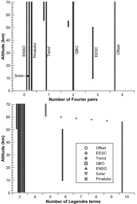
Fig. 1.(a) The number of Fourier pairs (N in equation 4 used to define the perturbation pattern for each basis

function fit coefficient. If this value is zero then no seasonality is included in the perturbation pattern. (b) The

number of terms included in the Legendre polynomial expansion of eachX2icoefficient in equation 4. Traces

are offset slightly from one another to avoid overlap.

pairs in the perturbation pattern very subtle changes in the mean annual cycle from one level to the

next can be accurately tracked. The number of Fourier pairs included in the perturbation pattern

for EESC is decreased at upper levels since the change in the seasonality of the ozone response to

EESC from one level to the next at these upper levels is small. For ENSO, the solar cycle, and the

Pinatubo eruption, including seasonal dependence in the fit coefficients did not significantly improve

the quality of the fit and resulted in over-fitting in some cases. Their effects on ozone were therefore

assumed to be independent of season.

The number of terms in the Legendre expansions constrain the latitudinal structure in the

pertur-bation pattern and therefore how much the latitudinal structure in the regression model fit coefficient

field can change from one level to the next. For the offset basis function, which describes the mean

annual cycle, 10 Legendre polynomials are used since the annual cycle is a very robust feature in

7

Figure 1. (a) The number of Fourier pairs (N in Eq. 4) used to

de-fine the perturbation pattern for each basis function fit coefficient. If this value is zero then no seasonality is included in the perturbation pattern. (b) The number of terms included in the Legendre polyno-mial expansion of each X2i coefficient in Eq. (4). Traces are offset

slightly from one another to avoid overlap.

of the ozone response to EESC from one level to the next at these upper levels is small. For ENSO, the solar cycle, and the Pinatubo eruption, including seasonal dependence in the fit coefficients did not significantly improve the quality of the fit and resulted in overfitting in some cases. Their effects on ozone were therefore assumed to be independent of season.

The number of terms in the Legendre expansions con-strain the latitudinal structure in the perturbation pattern, and therefore how much the latitudinal structure in the regres-sion model fit coefficient field can change from one level to the next. For the offset basis function, which describes the mean annual cycle, 10 Legendre polynomials are used since the annual cycle is a very robust feature in the data and this allows for the amplitude of the annual cycle to adapt to small changes in meridional structure from one level to the next. This is reduced to 5 Legendre terms at the upper levels

-150-100-50 -50 0 0 0 0 0 0 0 0 0 0 0 Season -90 -60 -30 0 30 60 90 L a ti tu d e ( d e g ) Jan Ozone = [C₀x

DU/ppb EESC

+C₁+ (a) Season -90 -60 -30 0 30 60 90 L a ti tu d e ( d e g ) Jan

A pattern resulting from fit coefficientsC2toCn

defining the Fourier and Legendre expansions

] x EESC + other terms

-150-100 -50 -50 0 0 0 0 0 0 0 0 0 0 0 Season -90 -60 -30 0 30 60 90 L a ti tu d e ( d e g ) Jan Ozone = [0.0039285 x

DU/ppb EESC -0.2367 + (b) -0.4 -0.3 -0.3 -0.3 -0.3 -0.3 -0.2 -0.2 -0.2 -0.2 -0.2 -0.2 -0.1 -0.1 -0.1 -0.1 -0.1 -0.1 -0.1 0 0 0 0 0 0 0 0 0.1 0.1 0.1 0.1 0.1 0.1 0.1 0.2

0.2 0.2

0.2 0.2 0.2 0.3 0.3 0.3 0 .3 Season -90 -60 -30 0 30 60 90 L a ti tu d e ( d e g ) Jan

] x EESC + other terms

Ozone = (c)

-1.2 -1.1-1-0.9-0.8-0.7-0.6

-0.6 -0.6 -0.5

-0.5

-0.5

-0.5 -0.5

-0.5 -0.4 -0.4 -0.4 -0.4 -0.4 -0.4 -0.3 -0.3 -0.3

-0.3 -0.3

-0.3 -0.2 -0.2 -0.2 -0.2 -0.2 -0.2 -0.2

-0.2 -0.2 -0.2

-0.1 -0.1 -0.1 -0.1 -0.1 -0.1 -0.1 0 0 0 0 0 0.1 0.1 Season -90 -60 -30 0 30 60 90 L a ti tu d e ( d e g ) Jan

x EESC + other terms

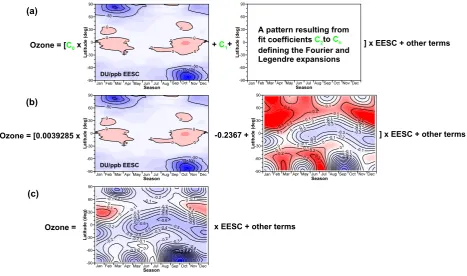
Fig. 2. A graphical illustration the derivation of the EESC fit coefficient, which is a function of latitude and

season, at 20 km. (a) The EESC coefficient is constructed as a first guess pattern response of ozone to EESC plus

an offset (C1) plus a perturbation that is constructed from Fourier and Legendre polynomials whose amplitudes

are fit coefficients in the linear least squares regression. The first guess pattern response in this case is taken

from fit coefficients from a regression model applied to total column ozone data. (b) Shows the situation after

the regression model has been fitted to the available ozone data at 20 km, while (c) shows the final EESC fit

coefficients resolved in latitude and season. Recall that because the regression model includes a trend term, the

assignment of variance to the EESC term may somewhat different to that expected; the positive (red) regions in

panel (c) are compensated by negative coefficients for the trend coefficient. The pattern shown in panel (c) then

becomes the first guess for the fits at 19 km and 21 km.

no longer being confined to the poles but spreading to lower latitudes. Note the factor 5 difference in

scales between panels (a) and (b). At 35 km increases in ozone are observed around mid-winter over

the Arctic and in late-winter/spring over the Antarctic, possibly indicative of increases in descent

over the poles. At 50 km there appears to be a positive trend in ozone in the Arctic early winter and 225

negative trends around mid-year over the tropics.

Figure 4 shows the summed contributions of the two QBO terms to ozone variability at four

indicative altitude levels. At 15 km the QBO induces large variability in Arctic ozone levels (up

to±0.4×1018 _molec/m3_{) and slightly smaller variability over the Antarctic. The ozone changes}

over the tropics are generally out of phase with the ozone changes over high latitudes though it 230

9

Figure 2. A graphical illustration the derivation of the EESC fit coefficient, which is a function of latitude and season, at 20 km. (a) The

EESC coefficient is constructed as a first guess pattern response of ozone to EESC plus an offset (C1) plus a perturbation that is constructed from Fourier and Legendre polynomials whose amplitudes are fit coefficients in the linear least squares regression. The first guess pattern response in this case is taken from fit coefficients from a regression model applied to total column ozone data. (b) Shows the situation after the regression model has been fitted to the available ozone data at 20 km, while (c) shows the final EESC fit coefficients resolved in latitude and season. Recall that because the regression model includes a trend term, the assignment of variance to the EESC term may be somewhat different than that expected; the positive (red) regions in (c) are compensated by negative coefficients for the trend coefficient. The pattern shown in (c) then becomes the first guess for the fits at 19 km and 21 km.

where changes from one level to the next are smaller. Sim-ilarly, for the EESC basis function, where it is necessary to track steep meridional gradients in the response of ozone to EESC, 6 Legendre polynomials are used at altitudes below 50 km, which is reduced to 3 at levels above 50 km. For all other basis functions, 3 Legendre terms are used in the pertur-bation pattern. This structure of the regression model results in up to 188 fit coefficients.

The advantage of using a first guess of the pattern response of ozone to the basis function is that the Fourier and Legendre expansions constituting the perturbation pattern can be trun-cated at fewer terms since steep gradients in season or lati-tude are likely to be captured by the first guess pattern. This prevents overfitting of the regression model which would likely cause anomalies in regions where there are fewer data to constrain the fit.

An illustrative example of how the first guess pattern and perturbation pattern combine to define the response of ozone to one of the basis functions is given in the next section.

4.3 Example of fit coefficient expansion

Consider, as an example, the structure of the B fit coefficient. This is shown schematically in Fig. 2 for the initial regression model fit at 20 km. The first guess field from the total column ozone regression model has units of DU per ppb of EESC. For ozone measured in ppm, the C0 coefficient (see Fig. 2) would then have units of ppm DU−1_{. All other C}

xcoefficients would have units of ppm ppb−1_{. Note that it is only the shape} of the first guess field that is important. Units/scaling are ir-relevant as this is absorbed into the C0coefficient. The per-turbation field resulting from the regression model fit shows greater sensitivity to EESC in the Antarctic winter and over the tropics than would be expected from total column ozone. Slightly weaker sensitivity is found over northern midlati-tudes. Recall that because the regression model also includes a linear trend term, a precise attribution of ozone sensitivity to EESC cannot be made.

15 km

25 km

35 km

50 km

Max=0.60x1018molec/m3

Min=-3.52x1018molec/m3

Max=4.73x1017molec/m3

Min=-6.24x1017

molec/m3

Max=3.83x1017molec/m3

Min=-2.90x1017

molec/m3

Max=1.10x1016molec/m3

Min=-1.40x1016

molec/m3

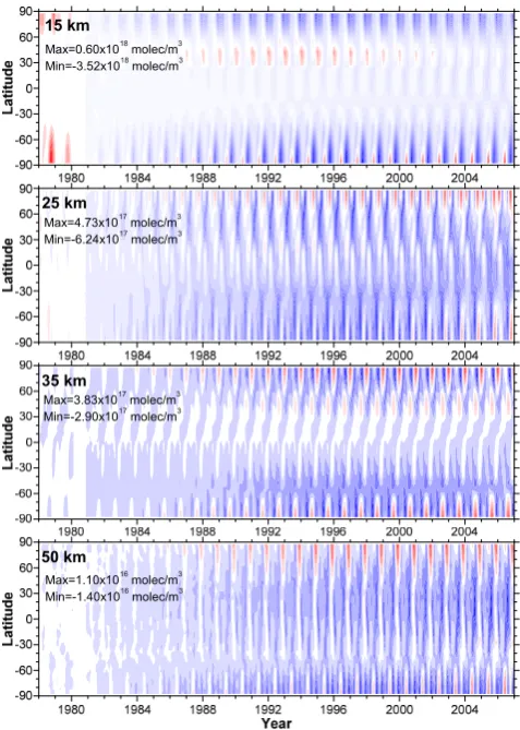
Fig. 3.The contribution of the trend and EESC basis functions to ozone variability, relative to a 1980 baseline,

at 4 indicative levels i.e 15, 25, 35 and 50 km. Red shows increases in ozone with respect to the 1980 baseline

while blue show decreases. The range of values is shown in each panel.

should be noted that in the tropics the 15 km altitude level is in the upper troposphere and below the

region where the QBO exerts a large influence on ozone. At 25 km the QBO exerts a large effect on

tropical ozone with an abrupt switch in phase at∼15◦. Sometimes the mid-latitude ozone anomalies

induced by the QBO extend to the pole but at other times the polar anomalies are anti-correlated

with the mid-latitude anomalies and positively correlated with the tropical anomalies. It is beyond 235

the scope of this paper to explore the mechanisms responsible for these differences in ozone response

to the QBO at different times. The QBO continues to influence ozone at 30 km altitude but in this

case the anomalies extend coherently (without a switch in phase) often to the poles, although with

some phase lag between the high and lower latitude anomalies. At 35 km the pattern is again similar

to that at 25 km showing equatorial anomalies of opposite sign to the anomalies poleward of∼15◦. 240

The ENSO contribution to ozone variance is small and is therefore not shown or described in detail

10

Figure 3. The contribution of the trend and EESC basis functions

to ozone variability, relative to a 1980 baseline, at four indicative levels, i.e., 15, 25, 35 and 50 km. Red shows increases in ozone with respect to the 1980 baseline while blue shows decreases. The range of values is shown in each panel.

5 Results from regression model fits

In this section examples of the contributions of different basis functions to ozone variability at different altitude levels are presented.

Figure 3 shows the combined contributions of the linear trend and EESC basis functions at four indicative levels. At 15 km the seasonal appearance of the Antarctic ozone hole in the latter part of each year is clearly evident, as is the win-tertime ozone depletion over the Arctic (though weaker than that over the Antarctic). Northern midlatitude ozone shows a small positive response, possibly in response to changes in dynamics, while small positive responses are also seen in the early winter at southern polar latitudes. At 25 km the pic-ture is more convoluted with wintertime ozone depletion no longer being confined to the poles but spreading to lower lat-itudes. Note the factor 5 difference in scales between pan-els (a) and (b). At 35 km increases in ozone are observed around midwinter over the Arctic and in late winter/spring

15 km

25 km

30 km

35 km

Fig. 4. The contribution of summed QBO basis functions to ozone variability, relative to a 1980 baseline, at 4

indicative levels i.e 15, 25, 30 and 35 km. Red regions shows increases in ozone with respect to the zero in the

QBO basis function while blue regions show decreases.

here.

Figure 5 shows the contribution of the Mt. Pinatubo volcanic eruption to ozone variability at four

indicative altitude levels. The pattern of response is determined, to some extent, by the prescribed

onset time (Bodeker et al., 2001a) for the Pinatubo basis function. At 15 km ozone over the polar

245

regions shows a response to the eruption within 1 year of the event. At 20 km, the ozone response

is hemispherically asymmetric providing some evidence for the causes of hemispheric differences

seen in the response of total column ozone to the eruption of the volcano (Bodeker et al., 2001). At

25 km equatorial ozone shows an almost immediate response to the eruption with weaker signals of

opposite sign over the poles. At 30 km ozone shows a weak positive response to the eruption over

250

the tropics. As alluded to above, these patterns may be affected by the initial, prescribed onset dates

for the Pinatubo basis function and should therefore not be over-interpreted.

11

Figure 4. The contribution of summed QBO basis functions to

ozone variability, relative to a 1980 baseline, at four indicative lev-els, i.e., 15, 25, 30 and 35 km. Red regions show increases in ozone with respect to the zero in the QBO basis function while blue re-gions show decreases.

over the Antarctic, possibly indicative of increases in descent over the poles. At 50 km there appears to be a positive trend in ozone in the Arctic early winter and negative trends around midyear over the tropics.

Figure 4 shows the summed contributions of the two QBO terms to ozone variability at four indicative altitude levels. At 15 km the QBO induces large variability in Arctic ozone levels (up to±0.4×1018_{molec m}−3_{) and slightly smaller} vari-ability over the Antarctic. The ozone changes over the tropics are generally out of phase with the ozone changes over high latitudes, though it should be noted that in the tropics the 15 km altitude level is in the upper troposphere and below the region where the QBO exerts a large influence on ozone. At 25 km the QBO exerts a large effect on tropical ozone with an abrupt switch in phase at∼15◦_{. Sometimes the} mid-latitude ozone anomalies induced by the QBO extend to the pole, but at other times the polar anomalies are anticorrelated

L

a

ti

tu

d

e

-0

.7

5

-0

.6

5

-0

.5

5

-0

.4

5

-0

.3

5

-0

.2

5

-0

.1

5

-0

.0

5

0

.0

5

0

.1

5

0

.2

5

0

.3

5

15 km

20 km

25 km

30 km

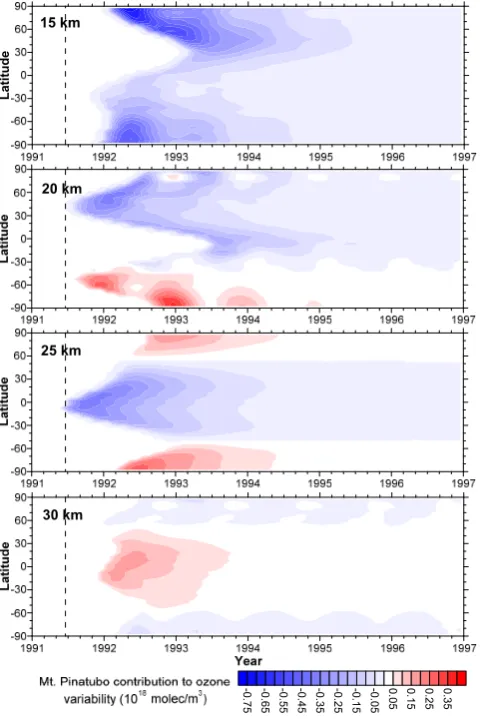
Fig. 5. The contribution of Mt. Pinatubo volcanic eruption to ozone variability at 15, 20, 25 and 30 km. Red

regions shows increases in ozone while blue regions show decreases.

6 Tier 1 ozone databases

Four different tiers of database were constructed as follows:

Tier 1.1 (Anthropogenic): Summing the contributions from the offset (A), EESC (B) and linear

255

trend (C) basis functions.

Tier 1.2 (Natural): Summing the contributions from the offset (A), QBO (DandE), ENSO (F), and

solar cycle (G) basis functions.

Tier 1.3 (Natural & Volcanoes): Summing the contributions from the offset (A), QBO (DandE),

ENSO (F), solar cycle (G), and Mt. Pinatubo volcanic eruption (H) basis functions.

260

Tier 1.4 (All): Summing the contributions from all basis functions.

These databases can then be used for different purposes e.g. to compare ozone radiative forcing

with and without the effects of changes in EESC and GHGs on ozone.

Examples of the Tier 0 and Tier 1.x databases for 3 selected latitude zones are shown in Figure

12

Figure 5. The contribution of Mt. Pinatubo volcanic eruption to

ozone variability at 15, 20, 25 and 30 km. Red regions show in-creases in ozone while blue regions show dein-creases.

with the midlatitude anomalies and positively correlated with the tropical anomalies. It is beyond the scope of this paper to explore the mechanisms responsible for these differences in ozone response to the QBO at different times. The QBO con-tinues to influence ozone at 30 km altitude, but in this case the anomalies extend coherently (without a switch in phase) often to the poles, although with some phase lag between the high and lower latitude anomalies. At 35 km the pattern is again similar to that at 25 km showing equatorial anoma-lies of opposite sign to the anomaanoma-lies poleward of∼15◦_{. The} ENSO contribution to ozone variance is small and is there-fore not shown or described in detail here.

Figure 5 shows the contribution of the Mt. Pinatubo vol-canic eruption to ozone variability at four indicative altitude levels. The pattern of response is determined, to some ex-tent, by the prescribed onset time (Bodeker et al., 2001a) for the Pinatubo basis function. At 15 km ozone over the polar regions shows a response to the eruption within 1 yr of the event. At 20 km the ozone response is

hemispheri-cally asymmetric, providing some evidence for the causes of hemispheric differences seen in the response of total column ozone to the eruption of the volcano (Bodeker et al., 2001b). At 25 km equatorial ozone shows an almost immediate re-sponse to the eruption with weaker signals of opposite sign over the poles. At 30 km ozone shows a weak positive re-sponse to the eruption over the tropics. As alluded to above, these patterns may be affected by the initial, prescribed onset dates for the Pinatubo basis function and should therefore not be overinterpreted.

6 Tier 1 ozone databases

Four different tiers of database were constructed as follows:

– Tier 1.1 (Anthropogenic): summing the contributions from the offset (A), EESC (B) and linear trend (C) basis functions.

– Tier 1.2 (Natural): summing the contributions from the offset (A), QBO (D and E), ENSO (F), and solar cycle (G) basis functions.

– Tier 1.3 (Natural and Volcanoes): summing the contri-butions from the offset (A), QBO (D and E), ENSO (F), solar cycle (G), and Mt. Pinatubo volcanic eruption (H) basis functions.

– Tier 1.4 (All): summing the contributions from all basis functions.

These databases can then be used for different purposes, for example, to compare ozone radiative forcing with and without the effects of changes in EESC and greenhouse gases on ozone.

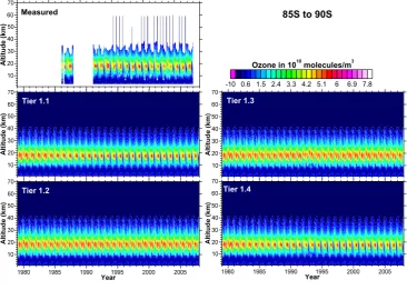
Examples of the Tier 0 and Tier 1.x databases for 3 se-lected latitude zones are shown in Fig. 6 (80◦_{N to 85}◦_N), Fig. 7 (0◦_{N to 5}◦_{N) and Fig. 8 (85}◦_{S to 90}◦_{S). It can be} seen that Tier 0 data are most frequently available in the tro-posphere and lower stratosphere, and more often in recent years than in earlier years. The Tier 0 data show consider-ably more variability than the Tier 1.4 data since the regres-sion model is not capable of tracking all of the variability in the Tier 0 data. Careful comparison of the Tier 1.1 and Tier 1.4 data shows the effects of natural variability and in partic-ular the effects of the QBO. Careful comparison of the Tier 1.2 and Tier 1.3 data shows the effects of the Mt. Pinatubo eruption. Over the South Pole (see Fig. 8), the onset of the Antarctic ozone hole is apparent in the Tier 0, Tier 1.1 and Tier 1.4 databases. Note, for example, in Tier 0 the almost complete absence of an ozone hole in 2002 as a result of the sudden stratospheric warming that year (Sinnhuber et al., 2003), which is not captured in the Tier 1.x databases since no basis functions are included in the regression model to track such variability. The option of using temperature as an explanatory variable in the regression model is discussed fur-ther in Sect. 8.

A

lt

it

u

d

e

(

k

m

)

85N to 80N

A

lt

it

u

d

e

(

k

m

)

Tier 1.2

Tier 1.1 Tier 1.3

Ozone in 1018molecules/m3

Tier 1.4

-10 0.6 1.5 2.4 3.3 4.2 5.1 6 6.9 7.8 Measured

Measured

Fig. 6. The Tier 0 ozone number densities between 80◦N and 85◦N (upper left panel marked ’Measured’ to

denote that these are the original monthly means), together with the Tier 1.1, 1.2, 1.3 and 1.4 time series.

6 (80◦N to 85◦N), Figure 7(0◦N to 5◦N) and Figure 8 (85◦S to 90◦S). It can be seen that Tier 0

265

data are most frequently available in the troposphere and lower stratosphere and more often in recent

years than in earlier years. The Tier 0 data show considerably more variability than the Tier 1.4 data

since the regression model is not capable of tracking all of the variability in the Tier 0 data. Careful

comparison of the Tier 1.1 and Tier 1.4 data shows the effects of natural variability and in particular

the effects of the QBO. Careful comparison of the Tier 1.2 and Tier 1.3 data shows the effects of the

270

Mt. Pinatubo eruption. Over the South Pole (see Figure 8) the onset of the Antarctic ozone hole

is apparent in the Tier 0, Tier 1.1 and Tier 1.4 databases. Note, for example, in Tier 0 the almost

complete absence of an ozone hole in 2002 as a result of the sudden stratospheric warming that year

(Sinnhuber et al., 2003) which is not captured in the Tier 1.x databases since no basis functions are

included in the regression model to track such variability. The option of using temperature as an

275

explanatory variable in the regression model is discussed further in Section 8.

The advantages gained from the logarithmic transformation of ozone (equation 2) are shown more

clearly in Figure 9. The very low ozone values during September and October inside the Antarctic

ozone hole of close to 0.1×1018_molec/m3_{are tracked well by the regression model without}

under-or over-estimating the values outside of the winter period.

280

13

Figure 6. The Tier 0 ozone number densities between 80◦

N and 85◦

N (upper left panel marked “Measured” to denote that these are the original monthly means), together with the Tier 1.1, 1.2, 1.3 and 1.4 time series.

A

lt

it

u

d

e

(

k

m

)

05N to 00N

A

lt

it

u

d

e

(

k

m

)

Tier 1.2

Tier 1.1 Tier 1.3

Ozone in 1018molecules/m3

Tier 1.4

-10 0.6 1.5 2.4 3.3 4.2 5.1 6 6.9 7.8 Measured

Measured

Fig. 7.As for Figure 6 but for 0◦N to 5◦N.

7 Validation

A further means of validating the database developed here is to compare vertically integrated ozone

profiles (ozone columns measured in Dobson Units (DU); 1DU=2.69×1016_molec/cm2_{) from the}

Tier 1.4 database with independent monthly mean total column ozone times series (see Figure 10).

The four monthly mean total column ozone time series shown in Figure 10 are updates of those

285

from Fioletov et al. (2002). Note that at no stage in the generation of the Tier 1.4 ozone database

are the values normalized to ensure agreement with an independent total column ozone value. The

integrated total column ozone from the Tier 1.4 database agrees well with the 4 independent time

series over the Arctic. The suppression of total column ozone following the eruption of Mt. Pinatubo,

seen in the independent observations, is tracked well, although the onset may be slightly too early.

290

Through the late 1990s and early 2000s the spring maximum in total column ozone is occasionally

under-estimated in the Tier 1.4 database, particularly in 1998, 1999, 2001, 2002, 2004 and 2006.

This under-estimation is likely the result of dynamically forced increases in ozone (Hadjinicolaou et

al., 2005) which cannot be tracked in the regression model since it does not include an appropriate

basis function.

295

Over the northern midlatitudes, the integrated Tier 1.4 time series tracks the independent total

14

Figure 7. As for Fig. 6 but for 0◦

N to 5◦ N.

A

lt

it

u

d

e

(

k

m

)

85S to 90S

A

lt

it

u

d

e

(

k

m

)

Tier 1.2

Tier 1.1 Tier 1.3

Ozone in 1018molecules/m3

Tier 1.4

-10 0.6 1.5 2.4 3.3 4.2 5.1 6 6.9 7.8

Measured

Measured

Fig. 8.As for Figure 8 but for 85◦S to 90◦S.

1980 1985 1990 1995 2000 2005

Year

0.1 1 10

O

z

o

n

e

(1

0

1

8m

o

le

c

/m

3)

Fig. 9. Monthly mean ozone at 16 km poleward of 85◦S. The Tier 0 monthly means are shown as black dots

while the Tier 1.4 reconstruction is shown as a blue line.

column ozone time series very well, but does shown some under-estimation of the spring-time peak

in many years. The suppression of ozone following the eruption of Mt. Pinatubo is captured well in

15

Figure 8. As for Fig. 8 but for 85◦

S to 90◦ S.

The advantages gained from the logarithmic transforma-tion of ozone (Eq. 2) are shown more clearly in Fig. 9. The very low ozone values during September and October inside the Antarctic ozone hole of close to 0.1×1018_{molec m}−3_are tracked well by the regression model without under- or over-estimating the values outside of the winter period.

7 Validation

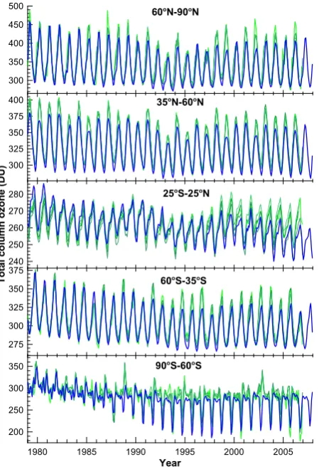
A further means of validating the database developed here is to compare vertically integrated ozone profiles (ozone columns measured in Dobson Units (DU); 1 DU=2.69× 1016_{molec cm}−2_{) from the Tier 1.4 database with} indepen-dent monthly mean total column ozone times series (see Fig. 10).

The four monthly mean total column ozone time series shown in Fig. 10 are updates of those from Fioletov et al. (2002). Note that at no stage in the generation of the Tier 1.4 ozone database are the values normalized to ensure agree-ment with an independent total column ozone value. The in-tegrated total column ozone from the Tier 1.4 database agrees well with the four independent time series over the Arctic. The suppression of total column ozone following the erup-tion of Mt. Pinatubo, seen in the independent observaerup-tions, is tracked well, although the onset may be slightly too early. Through the late 1990s and early 2000s, the spring maxi-mum in total column ozone is occasionally underestimated in the Tier 1.4 database, particularly in 1998, 1999, 2001, 2002, 2004 and 2006. This underestimation is likely the

re-A

lt

it

u

d

e

(

k

m

)

A

lt

it

u

d

e

(

k

m

)

Tier 1.2

Tier 1.1 Tier 1.3

Ozone in 1018molecules/m3

Tier 1.4

-10 0.6 1.5 2.4 3.3 4.2 5.1 6 6.9 7.8

Fig. 8.As for Figure 8 but for 85◦S to 90◦S.

1980 1985 1990 1995 2000 2005

Year

0.1 1 10

O

z

o

n

e

(1

0

1

8m

o

le

c

/m

3)

Fig. 9. Monthly mean ozone at 16 km poleward of 85◦S. The Tier 0 monthly means are shown as black dots

while the Tier 1.4 reconstruction is shown as a blue line.

column ozone time series very well, but does shown some under-estimation of the spring-time peak

in many years. The suppression of ozone following the eruption of Mt. Pinatubo is captured well in

15

Figure 9. Monthly mean ozone at 16 km poleward of 85◦_{S. The}

Tier 0 monthly means are shown as black dots while the Tier 1.4 reconstruction is shown as a blue line.

sult of dynamically forced increases in ozone (Hadjinicolaou et al., 2005) which cannot be tracked in the regression model since it does not include an appropriate basis function.

Over the northern midlatitudes, the integrated Tier 1.4 time series tracks the independent total column ozone time series very well, but does show some underestimation of the spring-time peak in many years. The suppression of ozone following the eruption of Mt. Pinatubo is captured well in the Tier 1.4 time series.

300 350 400 450 500

300 325 350 375 400

60o_N-90o_N

35o_N-60o_N

240 250 260 270 280

T

o

ta

l

c

o

lu

m

n

o

zo

n

e

(D

U

)

25o_S-25o_N

275 300 325 350 375

60o

S-35o

S

1980 1985 1990 1995 2000 2005

Year

200 250 300

350 90o_S-60o_S

Fig. 10. A comparison of zonal mean total column ozone from the four monthly mean observational time

series updated from Fioletov et al. (2002) shown in green traces, and zonal mean total column ozone calculated

by vertically integrating the Tier 1.4 database (blue trace). It is not necessary to distinguish between the 4

independent total column ozone time series and so these are not labelled individually.

the Tier 1.4 time series.

Over the tropics (25◦S to 25◦N) the integrated Tier 1.4 time series over-estimates total column 300

ozone by∼5 DU in the early part of the period and, after the late 1990s, under-estimates the ozone

resulting in a more negative trend than what is seen in the independent total column ozone time

series. The cause of this artifact is not known but likely results from a paucity of vertically resolved

ozone measurements in the tropics particularly in the early part of the period. The availability of

ozonesonde data from the SHADOZ programme (Thompson et al., 2003) significantly improves the 305

availability of data in this region and provides much needed measurements of ozone in the tropical

troposphere.

The integrated Tier 1.4 data track the independent total column ozone time series well over the

southern midlatitudes, but slightly over-estimate the spring-time peak in 1985 (again the result of

16

Figure 10. A comparison of zonal mean total column ozone from

the four monthly mean observational time series updated from Fio-letov et al. (2002) shown in green traces, and zonal mean total col-umn ozone calculated by vertically integrating the Tier 1.4 database (blue trace). It is not necessary to distinguish between the four inde-pendent total column ozone time series and so these are not labeled individually.

Over the tropics (25◦_{S to 25}◦_{N) the integrated Tier 1.4} time series overestimates total column ozone by∼5 DU in the early part of the period and, after the late 1990s, under-estimates the ozone resulting in a more negative trend than what is seen in the independent total column ozone time se-ries. The cause of this artifact is not known but likely results from a paucity of vertically resolved ozone measurements in the tropics, particularly in the early part of the period. The availability of ozonesonde data from the SHADOZ pro-gramme (Thompson et al., 2003) significantly improves the availability of data in this region and provides much needed measurements of ozone in the tropical troposphere.

The integrated Tier 1.4 data track the independent total column ozone time series well over the southern midlati-tudes, but slightly overestimate the springtime peak in 1985 (again the result of dynamical variability; see Bodeker et al., 2007), and slightly underestimate the springtime peak in 1991, 1994–1996, 2002, 2003 and 2005. The trend in

south-ern midlatitude ozone is expected to be captured well by the Tier 1.4 database.

Over the Antarctic, while the integrated Tier 1.4 time se-ries tracks the seasonal evolution of the Antarctic ozone hole, there is large intraseasonal variability which cannot be tracked by the regression model. In particular, the anoma-lously weak ozone hole in 2002 (Hoppel et al., 2003; Feng et al., 2005; Roscoe et al., 2005) is not reproduced in the Tier 1.4 database.

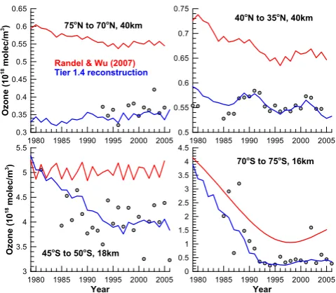
One of the vertically resolved ozone databases most com-monly used to constrain AOGCM simulations, to calcu-late ozone radiative forcing, and for analysis of long-term changes in the vertical distribution of ozone is the database of Randel and Wu (2007), hereafter referred to as R&W. This database, which extends from 1979 to 2005, derives interan-nual variations in ozone from the Stratospheric Aerosol and Gas Experiment (SAGE I and II) profile measurements, and from polar ozonesonde data from Syowa (69◦_{S) and} Res-olute (75◦_{N), and then adds these to the seasonally} vary-ing 1980 to 1991 ozone climatology of Fortuin and Kelder (1998) which is comprised entirely of ozonesonde data. As in the database presented here, a regression model is used to provide a globally filled database. March mean ozone val-ues from the Tier 0 and Tier 1.4 databases are compared with values extracted from R&W, at selected altitudes and latitude zones, in Fig. 11. In the tropical lower stratosphere, the Tier 1.4 data are significantly lower than the values from R&W, typically by a factor of 4. The interannual variabil-ity, forced primarily by the QBO, in the Tier 1.4 database and R&W track each other well outside of the polar regions (see, e.g., 40 to 45◦_{N at 30 km). The R&W database does} not include QBO variability poleward of 60◦_{. The Tier 1.4} database shows a more pronounced development of Arctic ozone depletion (see 80 to 85◦_{N at 16 km) than in the R&W} database, perhaps because the ozonesonde measurements at Resolute, used to derive the ozone anomalies used to con-struct the R&W database, may not always probe deep inside the Arctic vortex where ozone depletion is most severe. The solar cycle in ozone in the tropical upper stratosphere (see 10 to 15◦S at 40 km) is more pronounced in the Tier 1.4 database than in the R&W database.

Selected October mean times series from the Tier 0, Tier 1.4 and R&W databases are compared in Fig. 12. In some regions of the stratosphere (e.g., 70 to 75◦S at 40 km), the ozone number densities differ in magnitude (almost by a fac-tor of two) and the trends differ in sign. At the same alti-tude at northern midlatialti-tudes (35 to 40◦_{N), trends appear} to be similar but the R&W data are∼20 % higher than the values from the Tier 1.4 database. In the southern midlat-itude lower stratosphere (45 to 50◦_{S at 18 km), the R&W} database shows ozone staying approximately constant at∼ 5×1018_{molec m}−3_{, while the Tier 1.4 data show a decline} from that level around 1980 to∼4×1018_{molec m}−3_{over the} last decade of the database. The advantages of the logarith-mic transformation (see Eq. 2) are apparent in the Tier 1.4

1980 1985 1990 1995 2000 2005 4 4.5 5 5.5 6 6.5 7 7.5 O zo n e (1 0 1 8m o le c /m 3)

1980 1985 1990 1995 2000 2005 2.1 2.2 2.3 2.4 2.5 2.6 2.7 2.8 2.9 3

80o_{N to 85}o_{N, 16km 40}o

N to 45o

N, 30km

1980 1985 1990 1995 2000 2005 0.1 0.2 0.3 0.4 0.5 0.6 0.7 0.8 0.9 O z o n e (1 0 1 8m o le c /m 3)

1980 1985 1990 1995 2000 2005 0.45 0.5 0.55 0.6 0.65 0.7

0o_{N to 5}o_{N, 16km}

10o_{S to 15}o_{S, 40km}

Randel & Wu (2007) Tier 1.4 reconstruction

1980 1985 1990 1995 2000 2005 Year 2.2 2.3 2.4 2.5 2.6 2.7 2.8 O zo n e (1 0 1 8m o le c /m 3)

1980 1985 1990 1995 2000 2005 Year 0.4 0.45 0.5 0.55 0.6 0.65 0.7

45o_{S to 50}o_{S, 30km}

55o

S to 60o

S, 40km

Fig. 11. Selected March mean ozone time series from the Tier 0 database (grey dots), from Randel and Wu

(2007) (red trace) and from the Tier 1.4 database (blue trace).

We point the reader to Hassler et al. (2012) for a more thorough comparison of this database

against R&W, and the related database of Cionni et al. (2011).

8 Discussion and Conclusions

A new, global, gap free vertically resolved (1 km to 70 km altitude levels) ozone database has been 350

presented. The database is also available on pressure levels spaced approximately 1 km apart and

extending from 878.4 hPa to 0.046 hPa, and as both ozone mixing ratios and ozone number densities.

All four versions of the database (pressure/altitude and mixing ratio/number density), and all Tiers of

the database, are available at http://www.bodekerscientific.com/data/monthly-mean-global-vertically-resolved-ozone

and at http://dx.doi.org/10063/2437. The effects on the evolution of temperature changes in the trop-355

ical lower stratosphere when using this database to prescribe ozone boundary conditions in a climate

model are explored in Solomon et al. (2012).

The multiple satellite-based data sets, and the ozonesonde data, used to calculate the monthly

means that comprise the Tier 0 database were not corrected for offsets and drifts. Developing

meth-18

Figure 11. Selected March mean ozone time series from the Tier

0 database (grey dots), from Randel and Wu (2007) (red trace) and from the Tier 1.4 database (blue trace).

time series at 70 to 75◦S and 16 km, where the very low ozone values inside the Antarctic vortex are tracked well. The Tier 1.4 data also show less sign of ozone increases during the last decade of the period compared to R&W.

We point the reader to Hassler et al. (2012) for a more thorough comparison of this database against R&W, and the related database of Cionni et al. (2011).

8 Discussion and conclusions

A new, global, gap-free vertically resolved (1 km to 70 km altitude levels) ozone database has been pre-sented. The database is also available on pressure levels spaced approximately 1 km apart and extend-ing from 878.4 hPa to 0.046 hPa, and as both ozone mixing ratios and ozone number densities. All four versions of the database (pressure/altitude and mix-ing ratio/number density), and all tiers of the database, are available at http://www.bodekerscientific.com/data/ monthly-mean-global-vertically-resolved-ozone and at http://dx.doi.org/10063/2437. The effects on the evolution of temperature changes in the tropical lower stratosphere when

1980 1985 1990 1995 2000 2005 0.3 0.35 0.4 0.45 0.5 0.55 0.6 0.65 O z o n e (1 0 1 8m o le c /m 3)

1980 1985 1990 1995 2000 2005 0.5 0.55 0.6 0.65 0.7 0.75 75o

N to 70o

N, 40km 40

o_{N to 35}o_{N, 40km}

Randel & Wu (2007) Tier 1.4 reconstruction

1980 1985 1990 1995 2000 2005 Year 3 3.5 4 4.5 5 5.5 O z o n e (1 0 1 8m o le c /m 3)

1980 1985 1990 1995 2000 2005 Year 0 0.5 1 1.5 2 2.5 3 3.5 4 4.5

45o_{S to 50}o_{S, 18km}

70o

S to 75o

S, 16km

Fig. 12. Selected October mean ozone time series from the Tier 0 database (grey dots), from Randel and Wu

(2007) (red trace) and from the Tier 1.4 database (blue trace).

ods to detect and correct such inter-database discontinuities is the subject of ongoing work. In 360

this study the effects of any discontinuities are mitigated to some extent by calculating the Tier 0

monthly means in such a way that extreme outliers are discarded and by fitting a meridionally ’stiff’

regression model to all available data on a given altitude/pressure surface. However, the use of a

regression model also has the effect of not capturing all of the inter-annual variability in the Tier 0

data, in the Tier 1.x data. One possible means of capturing this variability would be to include zonal 365

temperature time series at each altitude/pressure level as basis functions. Since the model is never

used to attribute the origin of the variability, it does not matter whether the variance is assigned to

the newly introduced temperature time series basis functions or to other basis functions with similar

long-term structure. All that matters is that the variability is captured, that it can be projected to

regions outside of those where the regression model is trained, and that the regression model avoids 370

over-fitting the available data. An alternative to, or in addition to, temperature time series, eddy

heat fluxes, as a proxy for ozone transport, could be included as basis functions in the regression

model (Mader et al., 2007). Finally, while the integrated vertical columns are not normalized to an

independent total column ozone value, doing so might result in more realistic trend estimates from

the Tier 1.4 database and would result in better agreement with total column ozone trends. The 375

database would perhaps also be improved by a more sophisticated treatment of the Mt. Pinatubo

basis function and in particular better accounting for the shift in onset times for the Pinatubo basis

function and its dependence on latitude. Although the regression model produces uncertainties on

the fit coefficients (which are sensitive to both the uncertainties on the Tier 0 monthly means and also

the auto-correlation in the Tier 0 time series), these are not used here to generate uncertainties on 380

19

Figure 12. Selected October mean ozone time series from the Tier

0 database (grey dots), from Randel and Wu (2007) (red trace) and from the Tier 1.4 database (blue trace).

using this database to prescribe ozone boundary conditions in a climate model are explored in Solomon et al. (2012).

The multiple satellite-based data sets, and the ozonesonde data, used to calculate the monthly means that comprise the Tier 0 database were not corrected for offsets and drifts. De-veloping methods to detect and correct such inter-database discontinuities is the subject of ongoing work. In this study the effects of any discontinuities are mitigated to some ex-tent by calculating the Tier 0 monthly means in such a way that extreme outliers are discarded and by fitting a merid-ionally “stiff” regression model to all available data on a given altitude/pressure surface. However, the use of a re-gression model also has the effect of not capturing all of the interannual variability in the Tier 0 data, and in the Tier 1.x data. One possible means of capturing this variability would be to include zonal temperature time series at each altitude/pressure level as basis functions. Since the model is never used to attribute the origin of the variability, it does not matter whether the variance is assigned to the newly in-troduced temperature time series basis functions or to other basis functions with similar long-term structure. All that mat-ters is that the variability is captured, that it can be pro-jected to regions outside of those where the regression model is trained, and that the regression model avoids overfitting the available data. An alternative to, or in addition to, tem-perature time series, eddy heat fluxes, as a proxy for ozone transport, could be included as basis functions in the regres-sion model (Mader et al., 2007). Finally, while the integrated vertical columns are not normalized to an independent total column ozone value, doing so might result in more realis-tic trend estimates from the Tier 1.4 database and would re-sult in better agreement with total column ozone trends. The

database would perhaps also be improved by a more sophis-ticated treatment of the Mt. Pinatubo basis function and in particular better accounting for the shift in onset times for the Pinatubo basis function and its dependence on latitude. Although the regression model produces uncertainties on the fit coefficients (which are sensitive to both the uncertainties on the Tier 0 monthly means and also the auto-correlation in the Tier 0 time series), these are not used here to generate uncertainties on the Tier 1.4 databases. Tracking these un-certainties through the regression model, and incorporating them into the Tier 1.4 database, is also a focus of ongoing development of this database.

The regression model used to fill the database is cur-rently trained on measurements until 2006, although after the demise of HALOE and SAGE II in 2005, it is primarily ozonesonde data in 2006 that are used. To produce a database that extends until 2012, vertical ozone profile measurements from the GOMOS and OSIRIS measurements are planned to be added to the BDBP, which will then provide a new, ex-tended basis for the generation of new Tier 0 and Tier 1.4 databases.

Acknowledgements. We would like to thank Paul Newman for

providing the EESC time series and Bill Randel for access to the R&W database. We would also like to thank Susan Solomon for helpful discussions on the scope of this paper and on the potential importance of this new ozone database. This paper was developed as a contribution to the SPARC/IGACO/IO3C/NDACC (SI2N) initiative (http://igaco-o3.fmi.fi/VDO/index.html).

Edited by: R. Eckman

References

Austin, J., Tourpali, K., Rozanov, E., Akiyoshi, H., Bekki, S., Bodeker, G. E., Br¨uhl, C., Butchart, N., Chipperfield, M., Deushi, M., Fomichev, V. I., Giorgetta, M. A., Gray, L., Kodera, K., Lott, F., Manzini, E., Marsh, D., Matthes, K., Nagashima, T., Shibata, K., Stolarski, R. S., Struthers, H., and Tian, W.: Cou-pled chemistry climate model simulations of the solar cycle in ozone and temperature, J. Geophys. Res., 113, D11306, doi:10.1029/2007JD009391, 2008.

Bodeker, G. E., Scott, J. C., Kreher, K., and McKenzie, R. L.: Global ozone trends in potential vorticity coordinates using TOMS and GOME intercompared against the Dobson network: 1978–1998, J. Geophys. Res., 106, 23029–23042, 2001a. Bodeker, G. E., Connor, B. J., Liley, J. B., and Matthews, W. A.:

The global mass of ozone: 1978–1998, Geophys. Res. Lett., 28, 2819–2822, 2001b.

Bodeker, G. E., Garny, H., Smale, D., Dameris, M., and Deckert, R.: The 1985 Southern Hemisphere mid-latitude total column ozone anomaly, Atmos. Chem. Phys., 7, 5625–5637, doi:10.5194/ acp-7-5625-2007, 2007.

Cionni, I., Eyring, V., Lamarque, J. F., Randel, W. J., Stevenson, D. S., Wu, F., Bodeker, G. E., Shepherd, T. G., Shindell, D. T., and Waugh, D. W.: Ozone database in support of CMIP5 simulations:

results and corresponding radiative forcing, Atmos. Chem. Phys., 11, 11267–11292, doi:10.5194/acp-11-11267-2011, 2011. Daniel, J. S., Solomon, S., and Albritton, D. L.: On the evaluation

of halocarbon radiative forcing and global warming potentials, J. Geophys. Res., 100, 1271–1285, 1995.

Feng, W., Chipperfield, M. P., Roscoe, H. K., Remedios, J. J., Wa-terfall, A. M., Stiller, G. P., Glatthor, N., H¨opfner, M., and Wang, D.-Y.: Three-Dimensional Model Study of the Antarctic Ozone Hole in 2002 and Comparison with 2000, J. Atmos. Sci., 62, 822– 837, 2005.

Fioletov, V. E., Bodeker, G. E., Miller, A. J., McPeters, R. D., and Stolarski, R.: Global and zonal total ozone variations estimated from ground-based and satellite measurements: 1964–2000, J. Geophys. Res., 107, 4647, doi:10.1029/2001JD001350, 2002. Forster, P. M. d. F.: Radiative forcing due to stratospheric ozone

changes 1979-1997, using updated trend estimates, J. Geophys. Res., 104, 24395–24399, 1999.

Forster, P. M. d. F. and Shine, K. P.: Radiative forcing and temper-ature trends from stratospheric ozone changes, J. Geophys. Res., 102, 10841–10855, 1997.

Fortuin, J. P. F. and Kelder, H.: An ozone climatology based on ozonesonde and satellite measurements, J. Geophys. Res., 103, 31709–31734, 1998.

Hadjinicolaou, P., Pyle, J. A., and Harris, N. R. P.: The recent turnaround in stratospheric ozone over northern middle latitudes: A dynamical modeling perspective, Geophys. Res. Lett., 32, L12821, doi:10.1029/2005GL022476, 2005.

Hassler, B., Bodeker, G. E., and Dameris, M.: Technical Note: A new global database of trace gases and aerosols from multiple sources of high vertical resolution measurements, Atmos. Chem. Phys., 8, 5403–5421, doi:10.5194/acp-8-5403-2008, 2008. Hassler, B., Young, P. J., Portmann, R. W., Bodeker, G. E., Daniel,

J. S., Rosenlof, K. H., and Solomon, S.: Comparison of three ver-tically resolved ozone data bases: climatology, trends and radia-tive forcings, Atmos. Chem. Phys. Discuss., 12, 26561–26605, doi:10.5194/acpd-12-26561-2012, 2012.

Hoppel, K., Bevilacqua, R., Allen, D., Nedoluha, G. E., and Randall, C. E.: POAM III observations of the anomalous 2002 Antarctic ozone hole, Geophys. Res. Lett., 30, 1394, doi:10.1029/2003GL016899, 2003.

Kiehl, J. T., Schneider, T. L., Portmann, R. W., and Solomon, S.: Climate forcing due to tropospheric and stratospheric ozone, J. Geophys. Res., 104, 31239–31254, 1999.

M¨ader, J., Staehelin, J., Brunner, D., Stahel, W. A., Wohltmann, I., and Peter, T.: Statistical modeling of total ozone: Selection of ap-propriate explanatory variables, J. Geophys. Res., 112, D11108, doi:10.1029/2006JD007694, 2007.

Meehl, G. A., Stocker, T. F., Collins, W. D., Friedlingstein, P., Gaye, A. T., Gregory, J. M., Kitoh, A., Knutti, R., Murphy, J. M., Noda, A., Raper, S. C. B., Watterson, I. G., Weaver, A. J., and Zhao, Z.-C.: Global Climate Projections, in: Climate Change 2007: The Physical Science Basis. Contribution of Working Group I to the Fourth Assessment Report of the Intergovernmental Panel on Climate Change, edited by: Solomon, S., Qin, D., Manning, M., Chen, Z., Marquis, M., Averyt, K. B., Tignor, M., and Miller, H. L., Cambridge University Press, Cambridge, United Kingdom and New York, NY, USA, 2007.

Miller, R. L., Schmidt, G. A., and Shindell, D. T.: Forced annu-lar variations in the 20th century Intergovernmental Panel on