www.geosci-model-dev.net/4/483/2011/ doi:10.5194/gmd-4-483-2011
© Author(s) 2011. CC Attribution 3.0 License.
Geoscientific
Model Development
The CSIRO Mk3L climate system model version 1.0 – Part 1:
Description and evaluation
S. J. Phipps1,2,3,4, L. D. Rotstayn5, H. B. Gordon5, J. L. Roberts2,3,6, A. C. Hirst5, and W. F. Budd1,2,3
1Institute of Antarctic and Southern Ocean Studies, University of Tasmania, Australia 2Antarctic Climate & Ecosystems CRC, Hobart, Tasmania, Australia
3Tasmanian Partnership for Advanced Computing, Hobart, Tasmania, Australia 4Climate Change Research Centre, University of New South Wales, Australia
5Centre for Australian Weather and Climate Research: A partnership between CSIRO and the Bureau of Meteorology,
Aspendale, Victoria, Australia
6Australian Antarctic Division, Kingston, Tasmania, Australia
Received: 14 January 2011 – Published in Geosci. Model Dev. Discuss.: 1 February 2011 Revised: 31 May 2011 – Accepted: 7 June 2011 – Published: 17 June 2011
Abstract. The CSIRO Mk3L climate system model is a coupled general circulation model, designed primarily for millennial-scale climate simulations and palaeoclimate re-search. Mk3L includes components which describe the at-mosphere, ocean, sea ice and land surface, and combines computational efficiency with a stable and realistic control climatology. This paper describes the model physics and software, analyses the control climatology, and evaluates the ability of the model to simulate the modern climate.
Mk3L incorporates a spectral atmospheric general circula-tion model, az-coordinate ocean general circulation model, a dynamic-thermodynamic sea ice model and a land surface scheme with static vegetation. The source code is highly portable, and has no dependence upon proprietary software. The model distribution is freely available to the research community. A 1000-yr climate simulation can be com-pleted in around one-and-a-half months on a typical desktop computer, with greater throughput being possible on high-performance computing facilities.
Mk3L produces realistic simulations of the larger-scale features of the modern climate, although with some biases on the regional scale. The model also produces reasonable representations of the leading modes of internal climate vari-ability in both the tropics and extratropics. The control state of the model exhibits a high degree of stability, with only a weak cooling trend on millennial timescales. Ongoing de-velopment work aims to improve the model climatology and transform Mk3L into a comprehensive earth system model.
Correspondence to: S. J. Phipps
1 Introduction
The CSIRO Mk3L climate system model is a computationally-efficient atmosphere-land-sea ice-ocean general circulation model, designed for the study of climate variability and change on millennial timescales. It represents a new version of the CSIRO climate model, the history of which is described by Smith (2007). The atmosphere, land and sea ice models are reduced-resolution versions of those used by the CSIRO Mk3 coupled model (Gordon et al., 2002), which contributed towards CMIP3 (Meehl et al., 2007) and the IPCC Fourth Assessment Report (Solomon et al., 2007). The ocean model is taken from the CSIRO Mk2 coupled model (Gordon and O’Farrell, 1997), which contributed towards CMIP2 (Meehl et al., 2000) and the IPCC Third Assessment Report (Houghton et al., 2001). This combination produces a coupled climate system model that has both a realistic control climatology and very fast execution times.
efficiency allows new classes of scientific problems to be studied. Reduced-resolution models can be used, for ex-ample, to generate transient simulations of palaeoclimate epochs, to study the equilibrium response of the climate sys-tem to external forcings, or to carry out large ensembles of simulations.
The atmospheric component of Mk3L is a spectral gen-eral circulation model with a reduced horizontal resolution of R21. This gives zonal and meridional resolutions of 5.625◦ and∼3.18◦ respectively. A hybrid vertical coordinate is used, with 18 vertical levels. The model incorporates both a cumulus convection scheme and a prognostic stratiform cloud scheme. The radiation scheme simulates the full an-nual and diurnal cycles of longwave and shortwave radiation, and is able to calculate the cloud radiative forcings.
The land surface model employs a soil-canopy scheme and allows for 13 land surface and/or vegetation types and nine soil types. Prognostic soil and snow models describe the evo-lution of six soil layers and three snow layers, respectively. The vegetation types and land surface property distributions are pre-determined, however, and are therefore static.
The sea ice model includes both ice dynamics and ice ther-modynamics. A cavitating fluid rheology is used to rep-resent internal resistance to deformation, while the three-layer model of Semtner (1976) is used to represent the ther-modynamics of ice and snow. Fractional ice cover is per-mitted, representing the presence of sub-gridscale leads and polynyas.
The oceanic component of Mk3L is a coarse-resolution, rigid-lid,z-coordinate general circulation model. The hor-izontal grid matches the Gaussian grid of the atmosphere model, and there are 21 vertical levels. The prognostic vari-ables are potential temperature, salinity, and the zonal and meridional components of the horizontal velocity. The verti-cal velocity is diagnosed through the application of the conti-nuity equation. The scheme of Gent and McWilliams (1990) is used to parameterise the adiabatic transport of tracers by mesoscale eddies.
When coupled, the atmospheric and oceanic components exchange fields every hour, ensuring that the model simu-lates diurnal cycles of sea surface temperature and salinity. Flux adjustments are applied to improve the realism of the control climate, and to ensure that it is stable on millennial timescales.
The model can be run in three different configurations: (i) the fully-coupled climate system model, (ii) a stand-alone atmosphere-land-sea ice model, or (iii) a stand-alone ocean model. The latter two modes are used primarily for the pur-pose of spinning up the model.
The source code has been designed to ensure that Mk3L is portable across a wide range of computer architec-tures, whilst also being computationally efficient. Depen-dence on external libraries is restricted to the netCDF and FFTW libraries, both of which are freely available and open source, while a high degree of shared-memory parallelism
is achieved through the use of OpenMP directives. On an Intel Core 2 Duo processor, the coupled climate system model completes around 22 model years per day of walltime. Greater throughput can be achieved on high-performance computing facilities.
Mk3L is freely available to the research community for non-commercial purposes. A Subversion repository is used to manage the model distribution.
This paper describes version 1.0 of the CSIRO Mk3L cli-mate system model, analyses the control climatology, and evaluates the ability of the model to simulate the modern cli-mate. Section 2 describes the model physics, while Sect. 3 describes the model software and evaluates its computational performance. Section 4 describes the procedure used to ini-tialise the climate system model, and the climatology of the model is evaluated in Sect. 5. The simulated internal variabil-ity is evaluated in Sect. 6, and the drift in the mean climate state is examined in Sect. 7. Plans for future development are discussed in Sect. 8.
A companion paper analyses the response of the model to external forcings. User documentation, as well as further information regarding the initial development of Mk3L, is provided by Phipps (2006a).
2 Model description 2.1 Atmosphere model
The Mk3L atmosphere model is based on the atmospheric component of the CSIRO Mk3 coupled model (Gordon et al., 2002), but with the horizontal resolution reduced from spec-tral triangular T63 to specspec-tral rhomboidal R21. The zonal and meridional resolutions of the model physics grid are therefore 5.625◦and∼3.18◦respectively. The vertical reso-lution of 18 levels is retained.
The dynamical core of the atmosphere model is based upon the spectral method, and uses the flux form of the dy-namical equations (Gordon, 1981). Physical parameterisa-tions and non-linear dynamical flux terms are calculated on a latitude-longitude grid, with Fast Fourier Transforms used to map fields between their spectral and gridded forms. A fully-conservative semi-Lagrangian transport scheme is used to advect moisture (McGregor, 1993), while gravity wave drag is parameterised using the formulation of Chouinard et al. (1986).
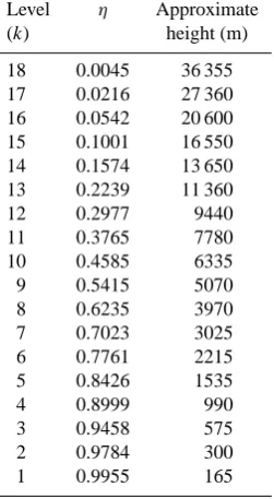
A hybrid vertical coordinate is used, which is denoted as theη-coordinate. As in theσ-system, whereσ is the ratio of the pressure to the surface pressure, the Earth’s surface forms the first coordinate surface. The remaining coordinate sur-faces then gradually revert to isobaric levels with increasing altitude. The 18 vertical levels used in the Mk3L atmosphere model are listed in Table 1 (Gordon et al., 2002, Table 1).
Table 1. The hybrid vertical levels used within the Mk3L atmo-sphere model: the value of theη-coordinate, and the approximate height.
Level η Approximate
(k) height (m)
18 0.0045 36 355
17 0.0216 27 360
16 0.0542 20 600
15 0.1001 16 550
14 0.1574 13 650
13 0.2239 11 360
12 0.2977 9440
11 0.3765 7780
10 0.4585 6335
9 0.5415 5070
8 0.6235 3970
7 0.7023 3025
6 0.7761 2215
5 0.8426 1535
4 0.8999 990
3 0.9458 575
2 0.9784 300
1 0.9955 165
Some adjustments are then made so as to avoid areas of sig-nificant negative elevation upon fitting to the truncated res-olution of the spectral model (Gordon et al., 2002). The re-sulting topography is shown in Fig. 1.
The radiation scheme treats solar (shortwave) and terres-trial (longwave) radiation independently. The default carbon dioxide concentration is 280 ppm, and the default ozone con-centrations are taken from the AMIP II recommended dataset (Wang et al., 1995). The model does not account for the ra-diative effects of other anthropogenic greenhouse gases. The method of Berger (1978) is used to calculate the Earth’s or-bital parameters. The default values of the epoch and the solar constant are 1950 CE and 1365 W m−2, respectively.
Full radiation calculations are conducted every two hours, allowing for both the annual and diurnal cycles. Clear-sky radiation calculations are also performed at each radiation timestep. This enables the cloud radiative forcings to be de-termined using Method II of Cess and Potter (1987), with the forcings being given by the differences between the radiative fluxes calculated with and without the effects of clouds.
The shortwave radiation scheme is based on the approach of Lacis and Hansen (1974), which divides the shortwave spectrum into 12 bands. Within each of these bands, the ra-diative properties are taken as being uniform. The longwave radiation scheme uses the parameterisation developed by Fels and Schwarzkopf (Fels and Schwarzkopf, 1975, 1981; Schwarzkopf and Fels, 1985, 1991), which divides the long-wave spectrum (long-wavelengths longer than 5 µm) into seven bands.
Fig. 1. The topography of the Mk3L atmosphere model: the elevation of land gridpoints (m).
The planetary boundary layer is described using a mod-ified version of the stability-dependent scheme of Louis (1979). The scheme of Holtslag and Boville (1993) is used to incorporate the nonlocal effects of large eddy transport.
The cumulus convection scheme is based on the UK Me-teorological Office scheme (Gregory and Rowntree, 1990), and generates both the amount and the liquid water content of convective clouds. This scheme is coupled to the prog-nostic cloud scheme of Rotstayn (1997, 1998) and Rotstayn et al. (2000), which calculates the amount of stratiform cloud using the three prognostic variables of water vapour mixing ratio, cloud liquid water mixing ratio and cloud ice mixing ratio.
Time integration is via a leapfrog time integration scheme, with a Robert-Asselin time filter (Robert, 1966) used to pre-vent decoupling of the time-integrated solutions at odd and even timesteps. A semi-implicit treatment of gravity waves increases the maximum permissible timestep duration. The main timestepping loop is executed once every 20 min, with the physics and dynamics calculations being conducted every timestep. However, full radiation calculations are only con-ducted once every six timesteps. At each of the intervening timesteps, the atmospheric heating rates are held constant, but the upward longwave and downward shortwave fluxes at the surface are re-calculated in order to smooth the diurnal cycle of net radiation.
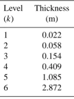
Table 2. The thickness of the soil layers used within the Mk3L land surface model.
Level Thickness
(k) (m)
1 0.022
2 0.058
3 0.154
4 0.409
5 1.085
6 2.872
2.2 Land surface model
The land surface model is an enhanced version of the soil-canopy scheme of Kowalczyk et al. (1991, 1994). A new parameterisation of soil moisture and temperature has been implemented, a greater number of soil and vegetation types are available, and a multi-layer snow cover scheme has been incorporated (Gordon et al., 2002). The land surface model uses the same horizontal grid and timestepping as the at-mosphere model. The zonal and meridional resolutions are therefore 5.625◦ and∼3.18◦, respectively, with a timestep
of 20 min.
The soil-canopy scheme allows for 13 land surface and/or vegetation types and nine soil types. The land surface property distributions are pre-determined, with seasonally-varying values being provided for the albedo and roughness length, and annual-mean values for the vegetation fraction. A seasonally-varying stomatal resistance is calculated by the model, subject to a specified minimum value. The soil model has six layers, the thicknesses of which are shown in Table 2. The total depth of the soil column at all gridpoints is 4.6 m. Soil temperature and the liquid water and ice contents are calculated as prognostic variables. Run-off occurs once the surface layer becomes saturated, and is assumed to travel in-stantaneously to the ocean via the path of steepest descent.
The snow model computes the temperature, snow density and thickness of three snowpack layers, as well as the snow albedo. The maximum snow depth is set at 4 m, with any excess snowfall being converted to run-off. When snow is present, the model also reduces the vegetation fraction for some vegetation types, to allow for vegetation being partially or completely buried by snow. Ice sheets are not explicitly represented, although there are land surface and soil types that reflect the presence of perennial ice cover.
2.3 Sea ice model
The sea ice model includes both ice dynamics and ice ther-modynamics, and is described by O’Farrell (1998). Internal resistance to deformation is parameterised using the cavitat-ing fluid rheology of Flato and Hibler (1990, 1992). The
thermodynamic component is based on the model of Semt-ner (1976), which splits the sea ice into three layers, one for snow and two for ice. Sea ice gridpoints are allowed to have fractional ice cover, representing the presence of sub-gridscale leads and polynyas. The sea ice model uses the same horizontal grid as the atmosphere model, and the zonal and meridional resolutions are therefore 5.625◦and∼3.18◦ respectively. A timestep of 1 h is used.
Ice advection arises from the forcing from above by atmo-spheric wind stresses, and from below by oceanic currents. When running as part of the coupled climate system model, the currents are obtained from the ocean model; in stand-alone mode, the currents are determined using a monthly climatology, with linear interpolation in time being used to estimate values at each timestep.
The advance and retreat of the ice edge in the stand-alone atmosphere-land-sea ice model is controlled by using a mixed-layer ocean model to compute water temperatures for those sea gridpoints which lie adjacent to sea ice (Gor-don et al., 2002). The mixed-layer ocean has a fixed depth of 100 m, and the evolution of the water temperature is de-termined using the surface heat flux terms and a weak relax-ation towards the prescribed sea surface temperature. The relaxation timescale used is 23 days. A mixed-layer ocean gridpoint can become a sea ice gridpoint either when its tem-perature falls below the freezing point of seawater, which is taken as being−1.85◦C, or when ice is advected into it from an adjacent sea ice gridpoint. When a mixed-layer ocean gridpoint is converted to a sea ice gridpoint, the initial ice concentration is set to 4 %. The neighbouring equatorward gridpoint, if it is a sea gridpoint, is then converted to a mixed-layer ocean gridpoint.
Surface processes can increase the ice thickness through the conversion of snow to ice. When the depth of the snow cover exceeds 2 m, the excess is converted into an equivalent amount of ice. Alternatively, when the weight of snow be-comes so great that the floe bebe-comes completely submerged, any submerged snow is converted into “white” ice. Surface processes can also reduce the ice thickness through melting and sublimation.
Lateral and basal ice growth and melt are determined by the temperature of the mixed-layer ocean. Additional ice can grow when the water temperature falls below the freezing point of seawater,−1.85◦C, subject to a maximum allowable thickness of 6 m. Once the water temperature rises above −1.5◦C, half of any additional heating is used to melt ice;
once it rises above−1.0◦C, all of the additional heating is
Table 3. The vertical levels used within the Mk3L ocean model: the thickness, the depth of the centre and base of each gridbox, and the value of the isopycnal thickness diffusivity.
Level Thickness Depth (m) κe
(k) (m) Centre Base (m2s−1)
1 25 12.5 25 0∗
2 25 37.5 50 70∗
3 30 65 80 180∗
4 37 98.5 117 290∗
5 43 138.5 160 420∗
6 50 185 210 580†
7 60 240 270 770†
8 80 310 350 1000‡
9 120 410 470 1000‡
10 150 545 620 1000‡
11 180 710 800 1000‡
12 210 905 1010 1000‡
13 240 1130 1250 1000‡
14 290 1395 1540 1000‡
15 360 1720 1900 1000‡
16 450 2125 2350 1000‡
17 450 2575 2800 1000‡
18 450 3025 3250 1000‡
19 450 3475 3700 1000‡
20 450 3925 4150 1000‡
21 450 4375 4600 1000‡
∗These values are fixed.
†These are the maximum allowable values; however, lower values may be specified by the user.
‡These are the default values; however, alternative values may be specified by the user.
2.4 Ocean model
The Mk3L ocean model is a coarse-resolution, rigid-lid,z -coordinate general circulation model, based on the oceanic component of the CSIRO Mk2 coupled model (Gordon and O’Farrell, 1997; Hirst et al., 2000; Bi et al., 2001, 2002). The CSIRO ocean model is, in turn, based on the implementation by Cox (1984) of the primitive equation numerical model of Bryan (1969).
The prognostic variables calculated by the model are po-tential temperature, salinity, and the zonal and meridional components of the horizontal velocity. The Arakawa B-grid (Arakawa and Lamb, 1977) is used, in which the tracer grid-points are located at the centres of the gridboxes and the hor-izontal velocity gridpoints are located at the corners. The vertical velocity is diagnosed through application of the con-tinuity equation, which enforces conservation of mass in an incompressible fluid.
The model uses a longitude-latitude grid, with walls at the north and south poles. The horizontal grid matches the Gaussian grid of the atmosphere model, such that the tracer gridpoints on the ocean model grid coincide with the
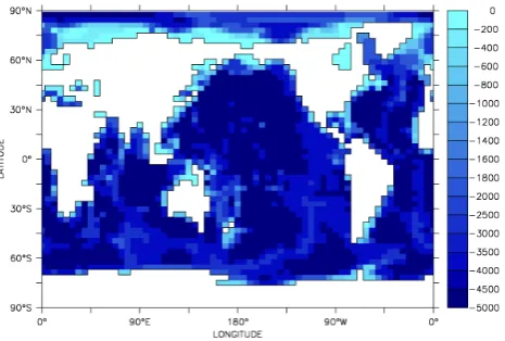
grid-Fig. 2. The bathymetry of the Mk3L ocean model: the depth of ocean gridpoints (m).
points on the atmosphere model physics grid. The zonal and meridional resolutions are therefore 5.625◦and∼3.18◦, re-spectively. There are 21 vertical levels, which are listed in Table 3.
The bottom topography is derived by interpolating the 1◦×1◦dataset of Gates and Nelson (1975b) onto the model grid, with some slight smoothing to ensure that a solution is achieved when calculating the barotropic streamfunction (Cox, 1984). The resulting bathymetry is shown in Fig. 2.
The land/sea mask used by the ocean model differs from that used by the atmosphere model. The tips of South America and the Antarctic Peninsula are removed, ensur-ing that Drake Passage accommodates three horizontal ve-locity gridpoints. To ensure adequate resolution of the Greenland-Scotland sill, Iceland is also removed; likewise, a re-arrangement of the land/sea mask ensures adequate reso-lution of the flows through the Indonesian archipelago. Sval-bard, which occupies a single isolated gridpoint on the at-mosphere model grid, is not represented in the ocean model. Any straits that have a width of only one gridpoint on the tracer grid are closed, as these will not contain any horizon-tal velocity gridpoints. The Bass, Bering, Gibraltar, Hudson and Torres Straits, the Mozambique Channel and the Sea of Japan are therefore removed, while the Canadian archipelago becomes a land bridge.
The bathymetry defines six basins which have no resolved connection with the world ocean: the Baltic, Black, Caspian and Mediterranean Seas, Hudson Bay and the Persian Gulf. With the exception of the Caspian Sea, each of these basins exchanges water with the world ocean via straits which are not resolved on the model grid. The effects of these ex-changes are parameterised within the model through an im-posed mixing between the gridpoints which lie to either side of each unresolved strait.
Table 4. The computational performance of the Mk3L coupled cli-mate system model: execution rates in model years per day of wall-time.
Processor type Number of cores
and speed 1 2 4 8
Intel Nehalem 2.93 GHz 15 28 48 74
Intel Xeon 3.0 GHz 14 22 33 50
Intel Core 2 Duo 3.0 GHz 13 22 − −
prevent decoupling of the time-integrated solutions at odd and even timesteps. Fourier filtering is used to reduce the timestep limitation arising from the CFL criterion (e.g., Washington and Parkinson, 1986) associated with the conver-gence of meridians at high latitudes, particularly in the Arctic Ocean (Cox, 1984). Fourier filtering is applied northward of 79.6◦N in the case of tracers, and northward of 81.2◦N in the case of horizontal velocities. The rigid-lid boundary condi-tion (Cox, 1984) is employed to remove the timestep limita-tion associated with high-speed external gravity waves. The ocean bottom is assumed to be insulating, while no-slip and insulating boundary conditions are applied at lateral bound-aries.
To reduce the execution time, the stand-alone ocean model employs an asynchronous timestepping scheme, with a timestep of 1 day used to integrate the tracer equations, and a timestep of 20 min used to integrate the momentum equa-tions. However, asynchronous timestepping distorts the rep-resentation of time-dependent features such as Rossby Waves (Bryan, 1984). Within the coupled climate system model – and during the final stage of spin-up runs, prior to cou-pling to the atmosphere-land-sea ice model – a synchronous timestepping scheme is therefore employed, with a timestep of 1 h used to integrate both the tracer and momentum equa-tions.
The vertical diffusivity varies as the inverse of the Brunt-V¨ais¨al¨a frequency, following the scheme of Gargett (1984). The minimum diffusivity is set to 3×10⁻⁵m2s−1, except in the upper levels of the ocean, where it is increased to sim-ulate the effects of mixing induced by surface winds. The minimum diffusivity between the upper two levels of the model is set to 2×10⁻³m2s−1, while that between the sec-ond and third levels is set to 1.5×10⁻⁴m2s−1. Whenever static instability arises, the vertical diffusivity is increased to 100 m2s−1, simulating convective mixing; convection is therefore treated as a purely diffusive process.
Diffusion of tracers along surfaces of constant neutral den-sity (isoneutral diffusion) is represented by the scheme of Cox (1987). In the default configuration of the model, the isoneutral diffusivity is set to the depth-independent value of 1000 m2s−1. No background horizontal diffusion is applied.
The adiabatic transport of tracers by mesoscale eddies is represented by the scheme of Gent and McWilliams (1990) and Gent et al. (1995). An eddy-induced horizontal transport velocity is diagnosed, which is added to the resolved large-scale horizontal velocity to give an effective horizontal trans-port velocity. The continuity equation can be used to derive the vertical component of either the eddy-induced transport velocity or the effective transport velocity. The default values for the isopycnal thickness diffusivity are shown in Table 3. Note that the values for levels 1 to 5 are fixed, and that up-per limits are imposed on the values for levels 6 and 7. This decrease in the isopycnal thickness diffusivity in the upper layers, with a value of zero at the surface, is required by the continuity constraint imposed on the eddy-induced transport (e.g., Danabasoglu et al., 2008).
In the stand-alone ocean model, the temperature and salin-ity of the upper layer are relaxed towards prescribed values for the sea surface temperature (SST) and sea surface salinity (SSS). The default relaxation timescale is 20 days. Instanta-neous values for the SST, SSS, and the zonal and meridional components of the surface wind stress, are determined from monthly climatologies, with linear interpolation in time be-ing used to estimate values at each timestep.
2.5 Coupled climate system model
Within the Mk3L coupled climate system model, the atmosphere-land-sea ice model (AGCM) and ocean model (OGCM) exchange fields every 1 h. This is in contrast to the approach employed by many other state-of-the-art cli-mate system models, whereby fields are exchanged only once per day (e.g., Collins et al., 2006). More frequent coupling allows the model to explicitly resolve diurnal cycles in sea surface temperature and salinity. In other models, this has been found to improve the simulated climate in the tropics, with enhancements that include better representation of dy-namical processes in the upper ocean, a reduction in the bi-ases in sea surface temperature, an enhanced seasonal cycle, and better representations of the Madden-Julian Oscillation and El Ni˜no-Southern Oscillation (Bernie et al., 2007, 2008; Danabasoglu et al., 2006).
Four fields are also passed from the AGCM to the OGCM: the surface heat and salt fluxes, and the zonal and merid-ional components of the surface momentum flux. The sur-face fluxes are averaged over the three consecutive AGCM timesteps, before being passed to the OGCM. There is no allowance for penetrative solar radiation, with all of the en-ergy supplied at the surface being added to the surface layer of the ocean. Mk3L employs a novel scheme to convert the surface freshwater flux to an equivalent salt flux, using the actual SSS at each gridpoint to perform the conversion, and applying a global offset to ensure conservation of freshwater (Phipps, 2006a).
Where there are mismatches between the positions of the coastlines on the AGCM and OGCM grids, spatial interpo-lation is used to estimate values of fields for locations where these fields are not defined on the source grid. Uniform off-sets are applied to the interpolated fields to ensure that the global integrals are conserved.
Flux adjustments are applied within the coupled model for two reasons: to improve the realism of the simulated cli-mate, and to minimise drift. Without them, the rate of climate drift is too large for the model to have utility on millennial timescales. The flux adjustments have a fixed annual cycle, and thus do not act to suppress internal variability. However, they arguably do limit the suitability of the model for study-ing climate states that represent large perturbations relative to the control state (Cubasch et al., 1992).
Following the approach of Sausen et al. (1988), adjust-ments are applied to each of the fluxes passed from the AGCM to the OGCM, and also to the SST and SSS. The need to apply adjustments to the surface velocities is avoided by employing a suitable spin-up procedure for the AGCM, whereby climatological values diagnosed from the OGCM are used.
3 Software and computational performance
The source code for Mk3L has been designed to ensure that the model is portable across a wide range of computer archi-tectures. It is written entirely in Fortran, with a high degree of shared-memory parallelism being achieved through the use of OpenMP directives. Dependence on external libraries is restricted to the netCDF and FFTW libraries, both of which are freely available and open source. It has been verified that the model will compile and run correctly on a wide variety of Intel-based architectures, as well as on the Compaq Alpha and SGI Origin scalar architectures, and on the CRAY SV1 and NEC SX6 vector architectures.
To maximise the computational performance of the model, Mk3L is compiled and executed as a single program, with the coupling routines integrated into the source code for each of the component models. This approach eliminates the inef-ficiencies that can arise from load imbalances and the over-heads associated with communication between different
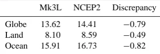
ex-Table 5. Annual-mean surface air temperature (◦C): Mk3L (av-erage for years 201–1200), NCEP2 (1979–2003 av(av-erage), and the model discrepancy (Mk3L minus NCEP2).
Mk3L NCEP2 Discrepancy
Globe 13.62 14.41 −0.79
Land 8.10 8.59 −0.49
Ocean 15.91 16.73 −0.82
ecutables. However, it contrasts with the more modular ap-proach employed by some other models (e.g., Collins et al., 2006), which compile and execute each component as a sep-arate program.
Table 4 shows the computational performance of the Mk3L coupled climate system model on typical state-of-the-art architectures for high-performance computing facilities (Intel Nehalem), servers (Intel Xeon) and desktop computers (Intel Core 2 Duo). The use of shared-memory parallelism, rather than distributed-memory parallelism, limits the num-ber of cores on which the model can be run. However, very fast execution times can still be achieved, with a 1000-yr cli-mate simulation able to be completed in as little as 13 days.
The Subversion revision control system is used to manage the model distribution. Mk3L is freely available to the re-search community, subject to the restriction that the model can only be used for non-commercial research purposes. Re-searchers can gain access to the Subversion repository by completing the online application form at http://www.tpac. org.au/main/csiromk3l/.
4 Spin-up procedure
A multi-stage spin-up procedure is used to initialise the Mk3L climate system model: (i) the atmosphere-land-sea ice and ocean models are integrated separately until they reach equilibrium, (ii) the surface fluxes diagnosed from each spin-up run are used to derive flux adjustments, (iii) the final states of each spin-up run are used to initialise the components of the climate system model, and (iv) the coupled climate sys-tem model is then integrated until it recovers from any initial adjustment. This section describes each stage of the proce-dure in detail.
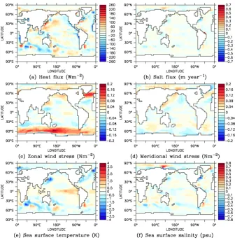
Fig. 3. The annual-mean values of the flux adjustments applied within the Mk3L coupled climate system model: (a) the surface heat flux, (b) the surface salt flux, (c, d) the zonal and meridional components of the surface wind stress, respectively, (e) the sea surface temperature, and (f) the sea surface salinity. For the surface fluxes, positive values indicate a downward flux.
4.1 Ocean model
The ocean model is first integrated to equilibrium. The model is initialised using the long-term annual-mean tem-peratures and salinities from the World Ocean Atlas 1998 dataset (Ocean Climate Laboratory, 1999), which is derived from observations spanning the period 1900–1997. It is then forced with climatological wind stresses derived from the NCEP-DOE Reanalysis 2 (Kanamitsu et al., 2002, hereafter referred to as NCEP2), while the temperature and salinity of the upper layer of the model are relaxed towards the World Ocean Atlas 1998 seasonal climatologies. The relaxation timescale used is 20 days.
The model is integrated for 4500 yr, using asynchronous timestepping for the first 4000 yr and synchronous timestep-ping thereafter. Between the penultimate and final centuries of the simulation, the magnitudes of the changes in the mean temperature and salinity on each model level do not ex-ceed 1.9×10⁻³K or 1.8×10⁻⁴psu, respectively. The final 100 yr are used to diagnose climatological surface fields for the purposes of deriving flux adjustments.
4.2 Atmosphere-land-sea ice model
The atmosphere-land-sea ice model is integrated to equilib-rium for pre-industrial conditions, using an atmospheric car-bon dioxide concentration of 280 ppm, a solar constant of 1365 W m−2, and modern (1950 CE) values for the Earth’s orbital parameters. World Ocean Atlas 1998 (Ocean Climate Laboratory, 1999) sea surface temperatures are applied as the bottom boundary condition, while the climatological ocean currents required by the sea ice model are diagnosed from the ocean model spin-up run.
The model is initialised from a previous spin-up run, and is integrated for 50 yr. The final 40 yr are used to diagnose climatological surface fields for the purposes of deriving flux adjustments.
4.3 Coupled climate system model
integrated for 4000 yr. The atmospheric carbon dioxide con-centration and solar constant are held constant at 280 ppm and 1365 W m−2, respectively, while modern values are used
for the Earth’s orbital parameters. Flux adjustments are ap-plied.
The first 200 yr of the simulation represent a spin-up pe-riod, and allow the model to recover from any initial adjust-ment. Years 201–1200 are used to characterise the control state of the model, and are analysed in Sects. 5 and 6. Later years are excluded from this analysis, so that it is not ex-cessively affected by any long-term trends exhibited by the model. The full 4000-yr simulation is used to characterise any drift in the mean climate state, and is examined in Sect. 7. 4.4 Flux adjustments
The flux adjustments applied within the coupled climate sys-tem model are derived by subtracting the climatological sur-face fields diagnosed from the ocean model spin-up run from those diagnosed from the atmosphere-land-sea ice model spin-up run. The resulting adjustments have a fixed annual cycle.
Figure 3 shows the annual-mean values of the adjustments that are applied within the coupled climate system model. Over the open ocean, the values of the adjustments are gen-erally small. Along the coastlines, heat flux adjustment terms arise from deficiencies in the representation of marine stra-tocumulus with the atmosphere model, and from the diffuse representation of the western boundary currents within the ocean model. Salt flux adjustment terms arise from discrep-ancies in the simulated rates of outflow for the major river systems, particularly the Amazon River. In the Southern Ocean, heat flux adjustment terms arise from the positioning of filaments of the Antarctic Circumpolar Current within the ocean model. Zonal wind stress adjustment terms arise from discrepancies between the strength of the Southern Hemi-sphere westerlies within the atmoHemi-sphere model and within NCEP2, which is used to spin up the ocean model. Sea sur-face temperature and salinity adjustment terms arise from er-rors in the climatology of the ocean model; the use of the relaxation surface boundary condition to spin up the model means that the simulation must differ from the prescribed cli-matology in order for the model to simulate non-zero values for the surface fluxes (Phipps, 2006b).
5 Mean climate
In this section, the control climatology of the model is anal-ysed, and the simulated mean climate is evaluated against ob-servational and reanalysis datasets. These datasets document the modern state of the climate, and discrepancies between the model and observations may therefore arise from the use of a pre-industrial scenario as the control state of the model. Discrepancies may also arise from the assumption that the
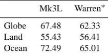
Table 6. Annual-mean total cloud cover (percent): Mk3L (average for years 201–1200) and the Warren climatology.
Mk3L Warren∗
Globe 67.48 62.33
Land 55.43 56.41
Ocean 72.49 65.01
∗The Warren climatology only covers 98.0 % of the Earth’s surface.
pre-industrial climate was in equilibrium with the contempo-rary boundary conditions. In reality, the large thermal iner-tia of the deep ocean, in combination with the time-varying nature of boundary conditions such as the Earth’s orbital pa-rameters, ensures that the climate system can only ever be in a state of quasi-equilibrium (Weaver et al., 2000).
5.1 Atmosphere
5.1.1 Surface air temperature
Figure 4a,b shows the simulated annual-mean surface air temperature, and compares it with NCEP2. The root-mean-square error is 1.90 K, with the model agreeing with the re-analysis to within 1 K over 56 % of the Earth’s surface, and to within 2 K over 85 % of the Earth’s surface. The only large-scale discrepancy is over Western Antarctica, where it is too cold.
Figure 4c–f shows the simulated mean surface air temper-atures for December-January-February (DJF) and June-July-August (JJA), and the discrepancies relative to NCEP2. The simulated winter temperatures over both polar regions are too cold, but otherwise the model is in good agreement with the reanalysis. The excessively warm winter temperatures over Hudson Bay are associated with the failure by the model to form sufficient sea ice cover in this region (Sect. 5.2).
The global-mean temperatures, and the means over land and over the ocean, are shown in Table 5. Although Mk3L is slightly cooler than NCEP2, the model was integrated for pre-industrial conditions while the NCEP2 values represent the 1979–2003 climatology. Indeed, the global-mean dis-crepancy of−0.79 K is consistent with the observed global-mean surface air temperature increase of 0.76±0.19 K be-tween 1850–1899 and 2001–2005 (Trenberth et al., 2007). 5.1.2 Cloud
Fig. 4. Surface air temperature (◦C), for Mk3L (average for years 201–1200) and NCEP2 (1979–2003 average): (a, c, e) Mk3L, annual, DJF and JJA means, respectively, and (b, d, f) Mk3L minus NCEP2, annual, DJF and JJA means, respectively.
Fig. 6. Annual-mean precipitation (mm/day): (a) Mk3L (average for years 201–1200), and (b) Legates and Willmott climatology v2.01.
the Western Pacific Ocean. The model also fails to reproduce the marine stratocumulus which is encountered in the north-eastern and north-eastern Pacific Ocean, and in the south-eastern Atlantic Ocean. These clouds are often poorly sim-ulated by climate models and yet, through reflection of sun-light, have a strong influence on the surface heat fluxes in these regions (Terray, 1998; Bretherton et al., 2004).
The global-mean cloud cover, and the means over land and over the ocean, are shown in Table 6. The model is in good agreement with the observed climatology over land, but the excess in the simulated cloud cover over the ocean is appar-ent.
5.1.3 Precipitation
Annual-mean precipitation is shown in Fig. 6 for Mk3L and version 2.01 of the observed climatology of Legates and Willmott (1990). The model is able to reproduce the large-scale features of the global distribution of precipita-tion, including the monsoonal precipitation associated with the South Pacific Convergence Zone.
Table 7. Annual-mean heat fluxes (W m−2, positive downward) at the top of the atmosphere, for Mk3L (average for years 201–1200) and ERBE (1985–1990 average).
Flux Mk3L ERBE
Outgoing shortwave radiation (60◦S–60◦N)
Net −102.14 −100.20
Clear sky −51.78 −49.81
Cloud forcing −50.36 −50.41
Outgoing longwave radiation (60◦S–60◦N)
Net −246.31 −242.90
Clear sky −279.49 −274.30
Cloud forcing +33.18 +31.39
However, there are some regional-scale biases. Over the Western Tropical Pacific and Indian Oceans, where the sim-ulated cloud cover is excessive, the simsim-ulated precipitation is also excessive. Over the Eastern Tropical Pacific, Indian and Atlantic Oceans, however, the simulated precipitation is deficient. The model is also too dry over the Indonesian archipelago and Central and Southwestern Australia. 5.1.4 Atmospheric temperature and winds
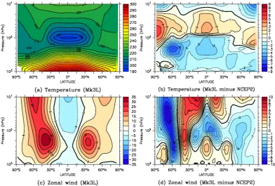
Figure 7 shows the zonal means of the simulated annual-mean atmospheric temperature and zonal wind speed, and compares them with NCEP2.
The model simulates the vertical distribution of temper-ature well, with both the tempertemper-ature and height of the minimum at the tropical tropopause being correctly simu-lated. However, there is a cool bias throughout the tropo-sphere, and a warm bias throughout the stratosphere. These biases are most pronounced over Antarctica, where the tropo-sphere is up to 8.9 K too cool and the stratotropo-sphere up to 5.4 K too warm. In the tropics, the biases in the simulated vertical profile of temperature do not exceed 3.7 K in magnitude.
Records derived from radiosondes and satellite-borne mi-crowave sounders indicate cooling of the stratosphere be-tween 1958 and 2004 of∼1.5 K, accompanied by a warm-ing of the troposphere of less than 0.5 K (Trenberth et al., 2007). This suggests that the warm bias in the simulated stratosphere is largely due to the use of pre-industrial green-house gas concentrations in the model, while the cool bias in the simulated troposphere is largely due to deficiencies in the model physics.
Fig. 7. The zonal means of annual-mean temperature (K) and annual-mean zonal wind speed (m s−1): (a, c) Mk3L (average for years 201– 1200), temperature and zonal wind speed, respectively, and (b, d) Mk3L minus NCEP2, temperature and zonal wind speed, respectively.
5.1.5 Radiation
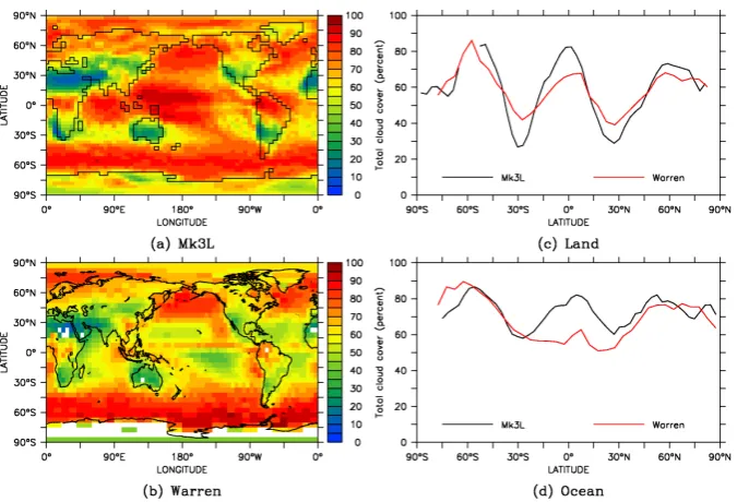
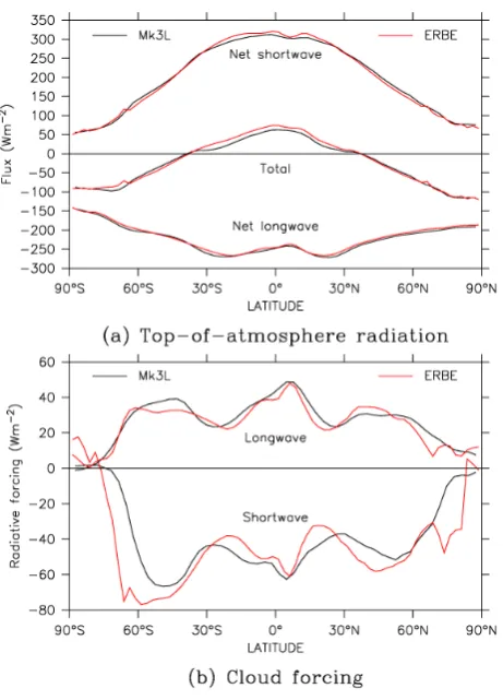
Figure 8a shows the zonal means of the annual-mean fluxes of shortwave and longwave radiation at the top of the atmo-sphere, for Mk3L and ERBE (the Earth Radiation Budget Experiment; Barkstrom, 1984). The model can be seen to simulate the zonal distribution of the radiative fluxes very well.
The zonal means of the annual-mean shortwave and wave cloud forcing are shown in Fig. 8b. The simulated long-wave cloud forcing is in good agreement with observations at all latitudes. There are discrepancies in the simulated short-wave cloud forcing at high latitudes, although it should be noted that the ERBE dataset is potentially unreliable over sea ice (Lubin et al., 1998).
Table 7 shows the annual-mean fluxes of outgoing short-wave and longshort-wave radiation at the top of the atmosphere. Because of the potential biases in the ERBE dataset at high latitudes, the comparison is restricted to the region 60◦S–
60◦N. The model slightly overestimates the magnitudes of
both the net outgoing fluxes of shortwave and longwave ra-diation at the top of the atmosphere. The excess of outgoing longwave radiation is due to deficient longwave absorption under clear-sky conditions. This is likely related, at least in part, to the use in the model of an atmospheric CO2
concen-tration appropriate for pre-industrial conditions. The magni-tude of the simulated shortwave cloud forcing is in excellent
agreement with observations, while the model slightly over-estimates the longwave cloud forcing.
5.2 Sea ice
The simulated seasonal cycles in the Northern and Southern Hemisphere sea ice extents and volumes are plotted in Fig. 9. Sea ice extents derived from the NOAA Optimum Interpola-tion (OI) sea surface temperature analysis v2 (Reynolds et al., 2002) are also shown; this analysis combines satellite ob-servations with in situ obob-servations from ships and buoys. The conventional definition of sea ice extent (e.g., Parkinson et al., 1999) is employed, namely that the sea ice extent is de-fined as the area over which the ice concentration is greater than or equal to 15 %.
The simulated annual cycle in ice extent is well simulated in both hemispheres. However, too much ice persists through the summer in the Northern Hemisphere, while too much ice forms in winter in the Southern Hemisphere. The simulated annual-mean sea ice extents in the Northern and Southern Hemispheres are 12.8×10¹²m2and 13.6×10¹²m2, respec-tively. These values are in good agreement with the observed extents of 12.2×10¹²m2and 13.2×10¹²m2, respectively.
Fig. 8. The zonal means of the annual-mean heat fluxes (positive downward) at the top of the atmosphere for Mk3L (black, average for years 201–1200) and ERBE (red, 1985–1990 average): (a) net shortwave, net longwave and total radiation, and (b) shortwave and longwave cloud forcing.
observations. However, the ice concentration is too low in Hudson Bay. In September, although the extent of the sea ice cover in the Arctic Ocean is again in good agreement with observations, the ice in Hudson Bay fails to melt. It is this deficiency that accounts for the excessive Northern Hemi-sphere sea ice extent in summer.
In the Southern Hemisphere, the extent of the sea ice cover is in reasonable agreement with observations. However, in September the ice cover extends slightly too far out from the coast at most longitudes, accounting for the excessive hemi-spheric sea ice extent in winter. The ice concentrations are also too low in both the Weddell and Ross Seas, with the re-sult that too little ice persists in these seas through the sum-mer.
The simulated March and September sea ice thicknesses are shown in Fig. 12. Observational datasets of ice thick-ness are limited in both spatial and temporal coverage. How-ever, Wadhams (2000), summarising the available data, in-dicates that ice thicknesses in the Arctic range from∼1 m in the sub-polar regions, such as Baffin Bay and the South-ern Greenland Sea, to∼7–8 m along the northern coasts of
Fig. 9. Sea ice extent (1012m2) and volume (1012m3): (a) sea ice extent for Mk3L (black, average for years 201–1200) and the NOAA OI analysis v2 (red, 1982–2003 average), and (b) sea ice volume for Mk3L.
Greenland and the Canadian archipelago. In Hudson Bay, the model forms excessively thick ice that persists through-out the year. As the ice concentration here is too low in win-ter, the model therefore appears to grow ice preferentially downwards, rather than outwards, in this region. However, the sea ice that forms elsewhere is much thinner. Compared to observational estimates, the simulated Arctic sea ice cover is therefore generally too thin.
Fig. 10. Northern Hemisphere sea ice concentration (percent): (a, b) Mk3L (average for years 201–1200), March and September, respec-tively, and (c, d), the NOAA OI analysis v2 (1982–2003 average), March and September, respectively. Values are only shown where the concentration is greater than or equal to 15 %.
5.3 Ocean
5.3.1 Water properties
The vertical profiles of potential temperature and salinity are shown in Fig. 13, for both Mk3L and the World Ocean Atlas 1998. The potential temperature represents the temperature that a volume of seawater would have if raised adiabatically to the surface. While the model prognoses the potential tem-perature, the World Ocean Atlas 1998 dataset contains in situ temperatures. These are therefore converted to potential tem-perature, using the multivariant polynomial method of Bry-den (1973).
The model ocean is too warm above 1400 m, but too cold at depth. It also has a consistent fresh bias, with the magnitude of the model discrepancy increasing with depth. Taking the average over the bottom five model levels, which span the depth range 2350–4600 m, the model is too cold by 1.09 K and too fresh by 0.27 psu.
Figure 14 shows the simulated zonal-mean potential tem-perature and salinity, and compares them with the World Ocean Atlas 1998. The model is too warm in the Arctic Ocean, and in the tropical and mid-latitude upper ocean. In contrast, it is too cold in the Southern Ocean and at depth. The simulated zonal-mean salinity exhibits a modest nega-tive bias at most latitudes and depths. A slight posinega-tive bias in the upper ocean in the Southern Hemisphere arises from the failure by the model to adequately simulate the formation of Antarctic Intermediate Water.
Fig. 11. Southern Hemisphere sea ice concentration (percent): (a, b) Mk3L (average for years 201–1200), March and September, respec-tively, and (c, d), the NOAA OI v2 (1982–2003 average), March and September, respectively. Values are only shown where the concentration is greater than or equal to 15 %.
5.3.2 Thermohaline circulation
The meridional overturning streamfunctions for the world ocean, and for the Atlantic and Pacific/Indian Oceans, are shown in Fig. 15; the rate of overturning is calculated by integrating both the large-scale and eddy-induced transport components. The rates of formation of North Atlantic Deep Water (NADW) and Antarctic Bottom Water (AABW) are 14.7 Sv and 11.8 Sv, respectively.
Observationally-based estimates of the rate of NADW for-mation lie within the range 15–20 Sv (Gordon, 1986), while those for the rate of AABW formation lie within the range 5–15 Sv (e.g., Gill, 1973; Carmack, 1977). The observed distribution of dissolved chlorofluorocarbons has also been used to produce estimated rates of NADW and AABW for-mation of∼17.2 Sv (Smethie and Fine, 2001) and∼8.1– 9.4 Sv (Orsi et al., 1999), respectively. The simulated rate of NADW formation is therefore slightly too weak, while the rate of AABW formation may be too strong.
Similar biases in the simulated rate of NADW forma-tion are encountered in other ocean models with compara-ble physics and spatial resolutions (e.g., England and Hirst, 1997; Hirst et al., 2000; Bi, 2002). As AABW is∼2 K colder than NADW (Orsi et al., 2001), the biases in the rate of deep water formation provide a possible explanation for the cold bias in the simulated deep ocean. This hypothesis is consis-tent with the fact that the cold bias arises from those regions of the world ocean that are ventilated by AABW (Fig. 14b). 5.3.3 Barotropic circulation
The annual-mean barotropic streamfunction is shown in Fig. 16. The Antarctic Circumpolar Current is evident, as are the mid-latitude gyres in the Atlantic, Pacific and Indian Oceans.
Fig. 12. Sea ice thicknesses for Mk3L (average for years 201–1200, cm): (a, b) Northern Hemisphere, March and September, respectively, and (c, d) Southern Hemisphere, March and September, respectively. The values shown are the mean thickness of sea ice where present, and are not weighted by the concentration. Values are only shown where the concentration is greater than or equal to 15 %.
(WOCE), estimate that the rate of transport is 136.7±7.8 Sv. Stammer et al. (2003), using an ocean global circulation model to assimilate WOCE data over the same period, es-timate that the rate of transport through Drake Passage is 124±5 Sv. The agreement between Mk3L and observations is particularly good when it is considered that other global ocean models simulate rates of transport through Drake Pas-sage which range from less than 100 Sv to more than 200 Sv (Olbers et al., 2004).
The simulated western boundary currents, however, are too weak and too diffuse. The maximum strength of the sim-ulated Gulf Stream, for example, is 24.4 Sv, whereas the ob-served strength is∼30.5 Sv (Schott et al., 1988). This prob-lem is encountered in coarse-resolution ocean models (e.g., Moore and Reason, 1993; Bi, 2002), and arises from the large horizontal viscosity which is required to ensure resolution of viscous boundary layers at the lateral walls (Bryan et al., 1975). For the configuration of the model analysed herein, the horizontal viscosity was set to 9×10⁵m2s−1.
6 Climate variability
In this section, the internal variability within the control simulation is analysed, and the simulated climate variabil-ity is evaluated against observational and reanalysis datasets. Analogously to the evaluation of the mean climate (Sect. 5), discrepancies may arise because of differences between the characteristics of modern natural climate variability and the natural climate variability that prevailed during the pre-industrial era.
Fig. 13. The zonal- and meridional-mean potential temperature and salinity for Mk3L (black, average for years 201–1200), and the World Ocean Atlas 1998 (red): (a) potential temperature, and (b) salinity.
of the simulated present-day El Ni˜no-Southern Oscillation, as well as the response to changes in the seasonal cycle of insolation (Kitoh et al., 2007; Brown et al., 2008). While a full analysis of the role of flux adjustments within Mk3L is beyond the scope of this paper, it is important to bear these caveats in mind when evaluating the simulated climate vari-ability.
6.1 Tropics
Figure 17 shows the leading principal component (PC) of the monthly sea surface temperature anomalies within the region 45◦S–45◦N, for Mk3L and for the HadISST1 observational analysis (Rayner et al., 2003).
In both the model and the analysis, El Ni˜no-Southern Os-cillation (ENSO; Philander, 1990) is the leading mode of variability in tropical sea surface temperatures. While the model successfully captures the overall spatial structure of the SST anomalies associated with ENSO, the location of greatest SST variability is located too far to the west. In the model, the largest anomalies in the equatorial Pacific Ocean occur at 163◦W whereas, in the analysis, they occur
at 113◦W.
The simulated ENSO variability is also too weak. In the model, the standard deviations of the monthly SST anoma-lies in the Ni˜no 3.4 (170◦–120◦W, 5◦S–5◦N) and Ni˜no 3 (150◦–90◦W, 5◦S–5◦N) regions are 0.51 K and 0.40 K, re-spectively. In contrast, the standard deviations for the period
1871–2003 according to the HadISST1 analysis are 0.76 K and 0.79 K, respectively. Thus the amplitude of the sim-ulated ENSO variability is 33 % weaker than the observed variability in the Ni˜no 3.4 region, and 50 % weaker than the observed variability in the Ni˜no 3 region. As the region of greatest SST variability is located too far to the west in the model, the simulated variability is particularly deficient in the Ni˜no 3 region.
The wavelet power spectra of the Ni˜no 3.4 SST anomaly, for both the model and for HadISST1, are shown in Fig. 18. Wavelet spectra were calculated using the method of Tor-rence and Compo (1998), modified following Liu et al. (2007) to ensure a physically consistent definition of energy. The observed power spectrum has peak variability at 3.6 yr, with a weak secondary maximum at 13.1 yr. The simulated power spectrum, however, has peak variability at 6.0 yr, with a secondary maximum of almost equal magnitude at 20.2 yr. The simulated ENSO has less power than observations at pe-riods shorter than 6 yr, and more power than observations on interdecadal timescales.
Within Mk3L, the simulated ENSO is therefore too weak, too slow, and characterised by excessive modulation on in-terdecadal timescales. The region of greatest SST variability is also located too far to the west. Such failings are typical of low-resolution coupled climate system models, such as those which participated in the Coupled Model Intercomparison Project (AchutaRao and Sperber, 2002). Higher-resolution models, such as those which contributed to the IPCC Fourth Assessment Report, are able to simulate ENSO variability more realistically (Guilyardi, 2006; Guilyardi et al., 2009). The deficiencies in the simulated ENSO variability within Mk3L are therefore likely to be a consequence of the reduced spatial resolution.
6.2 Extratropics
Fig. 14. The zonal-mean potential temperature (◦C) and salinity (psu) for the world ocean: (a, c) Mk3L (average for years 201–1200), and (b, d) Mk3L minus the World Ocean Atlas 1998.
Figure 19c,d shows the leading principal component of the monthly 500 hPa geopotential height anomalies for the Southern Hemisphere extratropics, defined here as the region 20◦–90◦S, for Mk3L and for NCEP2. The Southern
An-nular Mode (SAM, also known as the Antarctic Oscillation; Thompson and Wallace, 2000; Marshall, 2003) is the leading mode of variability in both the model and the analysis, with PC1 (PC2) explaining 23.4 % (8.3 %) and 17.6 % (10.8 %) of the variance in Mk3L and NCEP2, respectively. Although the model is able to capture the annular nature of the SAM, the simulated variability exhibits an excessive zonal symme-try. The largest negative geopotential height anomalies lie over Eastern Antarctica, with the model failing to resolve the dipole in variability in the Southern Pacific Ocean.
7 Climate drift
In a climate system model that is designed primarily for millennial-scale climate simulations, the rate of drift in the control state should be negligible. Mk3L employs fixed annual-cycle flux adjustments to minimise the rate of drift, as well as to improve the realism of the simulated climate. The adjustments are intended to prevent the mean states of the atmosphere, land surface, sea ice and ocean from drift-ing away from the states of the stand-alone models (Phipps, 2006b). This section examines the rate and nature of any residual drift that remains.
7.1 Surface air temperature
The evolution of the simulated global-mean surface air tem-perature (SAT) is shown in Fig. 20a. The model exhibits a slow but steady cooling trend, which becomes well es-tablished after year 1200. The global-mean SAT decreases 0.61 K by the end of the simulation, with the average rate of cooling being 0.015 K per century. There is no difference between the rates of change over land and over the ocean. 7.2 Sea ice
Figure 20b,c shows the evolution of the sea ice extent and volume in each hemisphere. Some initial adjustment during the first century of the simulation is apparent. In the Northern Hemisphere, this consists of the expansion of ice cover into Hudson Bay and the Labrador Sea (not shown), bringing the simulated ice cover into better agreement with observations. Thereafter, the Northern Hemisphere ice extent is relatively stable, increasing from 12.0 to 12.9×10¹²m2 between the
Fig. 15. Meridional overturning streamfunctions for Mk3L (aver-age for years 201–1200, Sv): (a) the world ocean, (b) the Atlantic Ocean, and (c) the Pacific/Indian Oceans.
the Caspian Sea for the first time (not shown). The Southern Hemisphere sea ice volume exhibits a steady upwards trend after year 500, increasing from 5.1 to 7.9×10¹²m3between the second and final centuries.
7.3 Sea surface temperature and salinity
The evolutions of the simulated global-mean sea surface tem-perature (SST) and sea surface salinity (SSS) are shown in Fig. 21. The drift in the simulated SST is similar to that in the simulated surface air temperature, with a steady cooling trend becoming established by year 1200. The global-mean SST decreases 0.44 K by the end of the simulation, with the average rate of cooling being 0.011 K per century. The simu-lated global-mean SSS exhibits a slow but steady freshening trend, decreasing 0.11 psu over the course of the simulation.
7.4 Oceanic circulation
Figure 22 shows the evolution in the rates of North Atlantic Deep Water (NADW) and Antarctic Bottom Water (AABW) formation, and in the rate of volume transport through Drake Passage. After some initial adjustment, the rates of deep water formation stabilise. Excluding the first century of the simulation, the mean rates of NADW and AABW formation are 14.4 and 11.9 Sv, respectively. The Antarctic Circumpo-lar Current (ACC), however, exhibits a slight strengthening trend, with the mean strength increasing from 146 to 160 Sv between the second and final centuries of the simulation. In the CSIRO Mk2 coupled model, the strength of the ACC has been shown to be sensitive to changes in the density struc-ture of the ocean interior (Bi, 2002). Such density changes, arising from the cooling trend in the Southern Ocean, may explain the ACC trend encountered here.
7.5 Summary
The control climate of the Mk3L coupled climate system model exhibits a high degree of stability on millennial timescales. Over the course of a 4000-yr control simulation, the global-mean surface air temperature cools at an average rate of just 0.015 K per century. This cooling trend is much smaller than that exhibited by the majority of models with comparable physics and spatial resolutions (Bell et al., 2000; Lambert and Boer, 2001). The drift exhibited by Mk3L is less, typically by between one and two orders of magnitude, than that exhibited by all seven of the non-flux-adjusted mod-els which participated in the Coupled Model Intercomparison Project (Lambert and Boer, 2001, Table 7), and by all but one of the eight models which employed flux adjustments. The only model to exhibit a smaller rate of drift was CSIRO Mk2, on which Mk3L is partly based.
The cooling trend exhibited by Mk3L is slow but con-sistent, and therefore respresents a source of concern. If the trends were to continue at the same rate as during the simulation presented here then, during a 10,000-yr simula-tion, global-mean surface air temperature would be expected to cool by ∼1.5 K, Southern Hemisphere sea ice volume would be expected to increase by∼140 %, and the Antarc-tic Circumpolar Current would be expected to strengthen by ∼25 %. Such rates of change would restrict the utility of the model for experiments which require very long integrations, such as the simulation of a full glacial cycle or a glacial-interglacial transition.
Fig. 16. The annual-mean barotropic streamfunction for Mk3L (average for years 201–1200, Sv).
Fig. 17. The leading principal component of the monthly sea sur-face temperature anomalies (K) for (a) Mk3L, years 201–1200, and (b) the HadISST1 analysis, 1871–2003.
by modifying the spin-up procedure, such that the coupled climate system model is initialised with more realistic sea ice cover.
Fig. 18. The wavelet power spectrum of the Ni˜no 3.4 sea surface temperature anomaly for Mk3L (black, years 201–1200) and the HadISST1 analysis (red, 1871–2003). Units are fraction of total power.
8 Future development
Future development work will address the deficiencies in the model climatology that have been identified herein. These deficiencies include both the biases in the control climatol-ogy, and the drift that is encountered within the coupled cli-mate system model.
Fig. 19. The leading principal component of the monthly 500 hPa geopotential height anomalies (m) for (a) Mk3L (years 201–1200, 20◦– 90◦N), (b) NCEP2 (1979–2003, 20◦–90◦N), (c) Mk3L (years 201–1200, 20◦–90◦S), and (d) NCEP2 (1979–2003, 20◦–90◦S).
be improved through enhancements to the model physics, while the simulated sea ice cover and deep ocean could be improved through the use of better spin-up procedures.
The deficiencies in the simulated El Ni˜no-Southern Os-cillation should also be addressed. Although this could be achieved through an increase in the spatial resolution, this would impact upon the computational performance. Expe-rience with other models has shown that a better represen-tation of ENSO can alternatively be achieved through im-provements to the parameterisation of atmospheric convec-tion (Neale et al., 2008), or through reducconvec-tions in the hor-izontal viscosity (Large et al., 2000) or vertical diffusivity (Meehl et al., 2001) used in the ocean.
Mk3L has a very stable control climatology, but there is a residual cooling trend that should be minimised. It is possi-ble that this could be achieved by initialising the model with more realistic sea ice cover. Furthermore, the stability of the control climatology is achieved partly through the use of flux adjustments. This is inherently undesirable, and future de-velopment efforts will seek to produce a non-flux-adjusted version of the model that nonetheless has a stable and realis-tic control climatology.
Ongoing development work also seeks to upgrade physical schemes within the model, and to incorporate representations of additional components of the earth system. Future ver-sions of Mk3L will include the CABLE land surface model (Kowalczyk et al., 2006), the CLM-DGVM dynamic global vegetation model (Levis et al., 2004), the ocean biogeochem-istry model of Matear and Hirst (2003), and the tropospheric aerosol scheme of Rotstayn et al. (2007). A dynamic ice sheet model (e.g., Rutt et al., 2009) and simulation of stable isotopes (e.g., Noone and Simmonds, 2002) are also being considered for incorporation. These developments will trans-form Mk3L from a climate system model into an earth sys-tem model. This will allow it to be used to address a whole new class of scientific questions, such as the role of vegeta-tion and carbon cycle feedbacks within the climate system, or the role of abrupt climate change.
9 Conclusions
Fig. 20. The drift in annual-mean surface air temperature, sea ice extent and sea ice volume: (a) surface air temperature, anomaly relative to the initial state, (b) sea ice extent, and (c) sea ice volume. The values shown are five-year running means.
Fig. 22. The rates of deep water formation, and the strength of the Antarctic Circumpolar Current: (a) the rates of formation of North Atlantic Deep Water (red) and Antarctic Bottom Water (green), and (b) the rate of volume transport through Drake Passage. The values shown are five-year running means.
representations of the atmosphere, ocean, sea ice and land surface. The model distribution is freely available to the re-search community.
The simulated surface air temperature, sea ice, cloud cover and precipitation exhibit broad agreement with observations. However, there are deficiencies in the Northern Hemisphere sea ice cover, associated with surface air temperatures which are too warm over Hudson Bay in winter. Other discrepan-cies in the simulated climate include excessive cloud cover over the tropical oceans, poor representation of marine stra-tocumulus, and regional biases in precipitation.
The simulated oceanic circulation is reasonable, with the strength of the Antarctic Circumpolar Current being in good agreement with observations. However, the rate of North At-lantic Deep Water formation is slightly too weak, the rate of Antarctic Bottom Water formation may be slightly too strong, and the western boundary currents are too weak and diffuse. The deep ocean is also too cold and too fresh.
The model produces reasonable representations of the leading modes of internal climate variability. The domi-nant mode of tropical climate variability is El Ni˜no-Southern Oscillation, although the simulated ENSO is too weak, too slow, and characterised by excessive modulation on inter-decadal timescales. The dominant modes of extratropical climate variability are the Northern and Southern Annular Modes. The geopotential height anomalies associated with each of these modes are reasonably well represented, al-though the simulated Southern Annular Mode exhibits an ex-cessive zonal symmetry.
The model is found to exhibit a high degree of stability, with the global-mean surface air temperature cooling at a rate of just 0.015 K per century over the course of a 4000-yr con-trol simulation. This drift arises from changes in the North-ern Hemisphere sea ice cover during the first century, and could potentially be avoided through improvements to the spin-up procedure. The strength of the thermohaline circu-lation exhibits no long-term trend.
Overall, the model has considerable utility for studying the behaviour of the larger-scale features of the climate system on millennial timescales. However, the reduced spatial res-olution leads to some regional scale biases and some defi-ciencies in the nature of the simulated interannual climate variability. The residual long-term drift also limits the utility of the model for very long climate simulations. Future devel-opment work will seek to address deficiencies in the model climatology and to incorporate representations of additional components of the earth system.
Appendix A