www.geosci-model-dev.net/5/869/2012/ doi:10.5194/gmd-5-869-2012
© Author(s) 2012. CC Attribution 3.0 License.
Geoscientific
Model Development
Land surface Verification Toolkit (LVT) – a generalized framework
for land surface model evaluation
S. V. Kumar1,2, C. D. Peters-Lidard2, J. Santanello2, K. Harrison2,3, Y. Liu2,3, and M. Shaw1,2,4
1Science Applications International Corporation, Beltsville, MD, USA
2Hydrological Sciences Laboratory, NASA Goddard Space Flight Center, Greenbelt, MD, USA 3Earth System Science Interdisciplinary Center, College Park, MD, USA
4Air Force Weather Agency, Offutt, NE, USA
Correspondence to: S. V. Kumar ([email protected])
Received: 1 December 2011 – Published in Geosci. Model Dev. Discuss.: 8 February 2012 Revised: 1 May 2012 – Accepted: 4 May 2012 – Published: 26 June 2012
Abstract. Model evaluation and verification are key in
im-proving the usage and applicability of simulation models for real-world applications. In this article, the development and capabilities of a formal system for land surface model evalu-ation called the Land surface Verificevalu-ation Toolkit (LVT) is described. LVT is designed to provide an integrated envi-ronment for systematic land model evaluation and facilitates a range of verification approaches and analysis capabilities. LVT operates across multiple temporal and spatial scales and employs a large suite of in-situ, remotely sensed and other model and reanalysis datasets in their native formats. In ad-dition to the traad-ditional accuracy-based measures, LVT also includes uncertainty and ensemble diagnostics, information theory measures, spatial similarity metrics and scale decom-position techniques that provide novel ways for performing diagnostic model evaluations. Though LVT was originally designed to support the land surface modeling and data as-similation framework known as the Land Information Sys-tem (LIS), it supports hydrological data products from non-LIS environments as well. In addition, the analysis of diag-nostics from various computational subsystems of LIS in-cluding data assimilation, optimization and uncertainty es-timation are supported within LVT. Together, LIS and LVT provide a robust end-to-end environment for enabling the concepts of model data fusion for hydrological applications. The evolving capabilities of LVT framework are expected to facilitate rapid model evaluation efforts and aid the definition and refinement of formal evaluation procedures for the land surface modeling community.
1 Introduction
Verification and evaluation are essential processes in the de-velopment and application of simulation models. Land sur-face models (LSMs) are one such class of simulation models specifically designed to represent the terrestrial water, energy and biogeochemical processes. LSMs generate estimates of terrestrial biosphere exchanges by solving governing equa-tions of soil-vegetation-snowpack medium, and can be run in either offline mode or coupled to an atmospheric model. An accurate representation of land surface processes is there-fore critical for improving models of the boundary layer and land-atmosphere coupling as well as real world applications, such as ecosystem modeling, agricultural forecasting and wa-ter resources prediction and management (NRC, 1996). The process of systematic evaluation and verification helps in the characterization of accuracy and uncertainty in the model predictions, which can then be used as a benchmark for fu-ture model enhancements. Further, quantitative measures of the fidelity of model simulations are essential for improving the usage and acceptability of LSM forecasts for real-world applications.
research, Entekhabi et al. (1999) emphasize the need for defining formal evaluation procedures to improve the “observability” of many LSM processes. For example, soil moisture in most LSMs represents an index of the moisture state (Koster et al., 2009) and the estimates from different models vary significantly even when forced with the same meteorology (Dirmeyer et al., 2006). Further, the soil profile representations in LSMs and assumptions about parameters such as soil hydraulic properties vary significantly across models. As a result, direct comparison of soil moisture esti-mates from these models against in-situ and remote sensing measurements becomes difficult. Given that a large suite of application models require soil moisture estimates as inputs, e.g., weather and climate forecasting (Fennessey and Shukla, 1999; Koster et al., 2004), agricultural models (Rosenzweig et al., 2002), ecosystem models (Friend and Kiang, 2005), it is important for the LSMs to generate observable estimates of soil moisture to avoid potential misinterpretations and incorrect usages. The development of a formal, systematic environment for model evaluation will help in bridging the gaps between the model and observations, and in improving the observability of LSM outputs.
Model performance is typically improved by either en-hancing the conceptual representations of processes (i.e., model physics) or by employing computational techniques (e.g., data assimilation, optimization, uncertainty algorithms, fuzzy logic) to augment model simulations. These computa-tional techniques provide the tools to exploit the information content in the observational data for improving model pre-dictions. The concept of “model data fusion” (MDF; Rau-pach et al., 2005; Williams et al., 2009) has been used to describe the paradigm of combining the information from models and available datasets. The key aspect of the MDF philosophy consists of using information from data to help the formulation, characterization and evaluation of models in a structured manner. The results of the evaluation step are then used to revise and improve model formulation and sub-sequent development. As part of the new structure formu-lated in 2009, the GLASS community has identified Bench-marking and MDF as two of its three core themes for research going forward. Here we describe the development of a for-mal evaluation system for land surface models that addresses both these themes identified by the GLASS community. The evaluation framework is designed to supplement an existing modeling system, to enable end-to-end formulations of the MDF paradigm.
As described in Kumar et al. (2006), Peters-Lidard et al. (2007) and Kumar et al. (2008a), the NASA Land Informa-tion System (LIS) is a flexible land surface modeling frame-work that has been developed with the goal of integrating satellite- and ground-based observational data products and advanced land surface modeling techniques to produce opti-mal fields of land surface states and fluxes. The LIS infras-tructure is designed as a land surface modeling and hydro-logical data assimilation system that generates estimates of
water and energy states (e.g., soil moisture, snow) and fluxes (e.g., evaporation, transpiration, runoff) over a range of spa-tial (as finely resolved as 1 km or finer) and temporal (up to 1 h and finer) resolutions. LIS operates several commu-nity land surface models and supports their application over global, regional or point domains. LIS is designed with ad-vanced software engineering principles and provides a flexi-ble, extensible framework for the inclusion of models, com-putational tools and datasets.
As a land surface modeling component for earth system models, LIS has also been coupled to atmospheric mod-els such as the Weather Research and Forecasting (WRF) model (Kumar et al., 2007; Santanello et al., 2009). LIS in-cludes a comprehensive data assimilation subsystem (Kumar et al., 2008b) that enables the incorporation of several ob-servational and satellite data sources for assimilation, in an interoperable manner. Additional computational tools to as-sist the utilization of data include parameter estimation and optimization (Santanello et al., 2007; Peters-Lidard et al., 2008; Kumar et al., 2012) and uncertainty modeling (Harri-son et al., 2012) subsystems. The uncertainty modeling com-ponents in LIS enable the explicit characterization of differ-ent sources of uncertainty in modeling using Bayesian infer-ence techniques. In summary, LIS provides several key com-ponents of the MDF paradigm, including a suite of LSMs and computational tools such as data assimilation, optimiza-tion and uncertainty estimaoptimiza-tion.
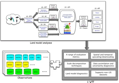
In this article, we describe the development of a formal system for land surface model evaluation called the Land sur-face Verification Toolkit (LVT), designed to enable the sys-tematic evaluation and intercomparison of various terrestrial hydrological datasets. LVT not only supports the diagnos-tic evaluation of the land model simulations from LIS and other land surface modeling systems, but also provides the capabilities for the analysis of outputs from various LIS sub-systems, such as data assimilation, optimization, uncertainty estimation, radiative transfer and emission models, and ap-plication models. A large suite of in-situ, remotely-sensed and other model and reanalysis datasets are supported in LVT, which captures a wide range of land surface and terres-trial hydrologic regimes across the globe. In addition, a wide range of analysis metrics and procedures are supported in LVT to facilitate a comprehensive evaluation of hydrological datasets. Figure 1 presents a schematic of the key functions of LVT and its interconnections with LIS and the observational datasets. The following sections describe the capabilities of LVT in detail.
Soil Moisture Evaporation Sensible Heat Flux
Runoff Snowpack properties Observations
Data Assimilation (DI,EnKF) LIS - DA
Land Surface Models (Noah, CLM, Catchment,
TESSEL, JULES)
LIS - LSM LIS - OPT
Optimization (LM, GA, SCE-UA)
Radiative Transfer Models (CMEM,CRTM)
LIS - RTM
Parameters
LIS - APP
LIS - Outputs
Meteorological Forecasts, Analysis,
Observations
Weather
Landslides
Floods
Drought LIS - UE
Uncertainty Estimation (MCMC,DEMC)
Parameters
Agriculture
FLUXNET SNOTEL ARM SCAN WMO
AMSR-E
MODIS ISCCP
AGRMET NLDAS SNODAS MERRA
....
....
....
Spatial and temporal upscaling/downscaling
Scale decomposition techniques A range of evaluation
metrics
Data assimilation and uncertainty diagnostics
Land model diagnostics Supports non-LIS datasets
Land model analyses
Observations
LVT
Fig. 1. Schematic of the Land surface Verification Toolkit and the association with the Land Information
System (LIS). LVT supports the analysis of outputs from various LIS subsystems. LIS-DA represents the data
assimilation subsystem, LIS-RTM represents the radiative transfer models within LIS, LIS-OPT represents the
optimization subsystem, LIS-UE represents the uncertainty estimation subsystem, LIS-LSM represents the land
surface models, and LIS-APP represents the various application models within LIS.
26
Fig. 1. Schematic of the Land surface Verification Toolkit and the association with the Land Information System (LIS). LVT supports the analysis of outputs from various LIS subsystems. LIS-DA represents the data assimilation subsystem, LIS-RTM represents the radiative transfer models within LIS, OPT represents the optimization subsystem, UE represents the uncertainty estimation subsystem, LIS-LSM represents the land surface models, and LIS-APP represents the various application models within LIS.
model testing and diagnostic evaluation, LVT completes the requisite components of the MDF paradigm.
This article is structured as follows: Sect. 2 provides a re-view of the land model evaluation and verification efforts. This is followed by the description of LVT design (Sect. 3) and features (Sect. 4). A number of examples are presented in Sect. 5 that demonstrate how the LVT capabilities enable end-to-end MDF experiments.
2 Background
There have been a number of efforts to document and stan-dardize land surface model evaluation. The model process development studies are typically focused on evaluating the model performance at point or local scales (e.g., Sellers et al., 1995; Chen et al., 1996; Pitman and Henderson-Sellers, 1998; Koren et al., 1999; Blyth et al., 2010; Barlage et al., 2010; Niu et al., 2011). Though they are instrumental in benchmarking the improvements to model physics, these re-ported enhancements do not necessarily translate to broader spatial scales. Blyth et al. (2011) stresses that the model eval-uations must be performed separately at the scales of interest, to guarantee transferability of model processes to different scales.
LVT Core
Time
Management Logging andDiagnostic Configuration TransformationGeospatial I/O
Management
Co
re
Structur
e
and
Fea
tur
es
Abs
tra
cti
ons
Us
e
Ca
seImpl
ementa
tio
ns FLUXNET fluxes
ARM fluxes, soil moisture, temperature SNOTEL snow water equivalent
AMSR-E soil moisture MODIS snow cover ISCCP surface temperature
USGS streamflow SURFRAD radiation CPC precipitation analysis
... FLUXNET fluxes ARM fluxes, soil moisture,
temperature SNOTEL snow water equivalent
AMSR-E soil moisture MODIS snow cover ISCCP surface temperature
USGS streamflow SURFRAD radiation CPC precipitation analysis
... FLUXNET fluxes ARM fluxes, soil moisture,
temperature SNOTEL snow water equivalent
AMSR-E soil moisture MODIS snow cover ISCCP surface temperature
USGS streamflow SURFRAD radiation CPC precipitation analysis
... Accuracy measures (RMSE, Bias, Correlation)
Ensemble measures (Likelihood) Uncertainty measures (Importance) Information theory measures (Entropy,
complexity)
Scale decomposition (Wavelet analysis) ...
Accuracy measures (RMSE, Bias, Correlation) Ensemble measures (Likelihood) Uncertainty measures (Importance) Information theory measures (Entropy,
complexity)
Scale decomposition (Wavelet analysis) ...
Accuracy measures (RMSE, Bias, Correlation) Ensemble measures (Likelihood) Uncertainty measures (Importance) Information theory measures (Entropy,
complexity)
Scale decomposition (Wavelet analysis) ...
Analysis
metrics Observations
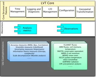
Fig. 2.Three-layer software architecture of Land surface Verification Toolkit (LVT)
27
Fig. 2. Three-layer software architecture of Land surface Verification Toolkit (LVT).
in-situ and remote sensing measurements are presented in Rodell et al. (2004a) and Kato et al. (2007). The LandFlux-EVAL project, a more recent initiative, evaluated evapotran-spiration estimates from a number of LSMs against in-situ data based estimates (Jiminez et al., 2011). Approaches to define a minimum acceptable performance benchmark of LSMs by comparing them to calibrated noncausal (statisti-cal/correlational) models are explored in Abramowitz et al. (2008). Though these efforts cover a wide spectrum of model evaluation and benchmarking of model process advance-ments, the evaluation criteria and the performance metrics tend to be specific to each application. LVT consolidates the requirements identified in these efforts within a single frame-work.
A number of software environments for conducting model verification has been reported in the literature. The Ensem-ble Verification System (EVS; Brown et al., 2010) developed at the US National Oceanic and Atmospheric Administra-tion’s (NOAA) Office of Hydrologic Development (OHD) provides an environment to verify ensemble forecasts of hydrologic and atmospheric variables such as precipitation, temperature and streamflow, and is used by forecasters at the US River Forecast Centers (RFCs). Protocol for the Anal-ysis of Land Surface models (PALS) is a web-based appli-cation for evaluating land surface models against observed datasets and calibrated statistical models (Abramowitz et al., 2008). LVT and PALS will continue to be developed con-currently to address community goals for benchmarking and MDF. Model Evaluation Toolkit (MET; Brown et al., 2009)
is a system developed by the Developmental Testbed Cen-ter (DTC) for the numerical weather prediction community to evaluate model performance. MET includes several methods for the diagnostic and spatial verification of NWP model out-puts. However, MET requires that the input datasets (model output and the observational data) be reformatted to certain predefined file formats. LVT shares many features with these existing environments, but focuses on the native use of obser-vational and model data sets, since the interpretation of the data formats and reporting procedures is a critical and time consuming step in the evaluation process. LVT is designed as a framework that can be directly used and extended by the individual users and also includes a number of advanced fea-tures such as the evaluation of data assimilation diagnostics, standardized land surface diagnostics and uncertainty and in-formation theory based analysis features. The following sec-tions describe the design and capabilities of LVT.
3 Design of the LVT framework
implementing new observational data sources and analysis metrics. The Abstractions layer provides the entry points for the reuse of existing generic capabilities of the LVT core. The top two layers thus represent the classic “semi-complete” na-ture of an object oriented framework, which is made fully functional by including specific implementations of the ab-stractions. As shown in Fig. 2, implementations to read and process observations from a wide range of terrestrial hydro-logical observations have been implemented using the
“Ob-servations” abstraction. Similarly, a large suite of analysis
metrics has been implemented by extending the “Metrics” abstraction.
LVT software is primarily written in Fortran 90 program-ming language. Though Fortran 90 lacks the direct support for object oriented programming concepts such as polymor-phism and inheritance, these properties can be simulated in software (Decyk et al., 1997) through the combined use of Fortran 90 and C programming languages. The compile-time polymorphism in LVT is simulated through the use of vir-tual function tables, by employing C language to interface with Fortran 90 functions, and by storing them in memory to be invoked at runtime. These virtual function tables enable the “Abstractions” layer constructs mentioned in the previ-ous paragraph.
A key advantage of this object oriented-based design is interoperability. The top two layers (LVT core and Abstrac-tions) define the interactions between an Observation or a
Metric implementation with the LVT core in a generic
man-ner. Similarly, the required interconnections between an
Ob-servation implementation and a Metric implementation are
also handled generically. As a result, the existing function-alities of the system are automatically available to a new addition in LVT, implemented through the extension of an Abstraction. For example, a newly incorporated observation implementation can take advantage of all available analysis metrics without having to define any additional interconnec-tions between each bottom layer component.
Note that many of the model-independent capabilities within the LVT are enabled by the Earth System Model-ing Framework (ESMF; Hill et al., 2004). ESMF provides a structured collection of building blocks that can be cus-tomized to develop model components for Earth Science ap-plications. It provides an infrastructure of utilities and a su-perstructure for coupling different model components. LVT employs the ESMF infrastructure utilities to handle the man-agement of clock/time, configuration, and logging. Further, LVT also employs the generic ESMF objects (called ESMF States) for sharing data and information between different components.
4 Capabilities of LVT
A critical part of an evaluation procedure is the processing of datasets, which normally consists of model outputs and
measurements from in-situ, satellite and remote sensing plat-forms. These datasets typically have different file formats, spatial and temporal scales and reporting procedures. Fur-ther, the in-situ and remotely sensed measurements typically require extensive quality control before their use. The rec-tification of such differences between datasets being com-pared is an essential, but routine and time consuming step in the evaluation process. The philosophy in LVT is to use the datasets in their native formats. The “plugin” style design of LVT enables the development of data processors correspond-ing to each dataset. Once developed, these data processors can be subsequently used to work with an ongoing data col-lection without additional reprocessing. Though the empha-sis on the use of native formats is useful for rapid use of the datasets, the use of high resolution datasets could be compu-tationally limiting, especially when the analysis is conducted against a coarse resolution model simulation. To circumvent this limitation, LVT provides a “data processing” run mode, where it performs various data handling operations (read, in-terpolation, reprojection and subsetting) and outputs the pro-cessed data to disk. The propro-cessed data can then be used by a subsequent analysis run of LVT.
4.1 Support for terrestrial hydrological datasets in LVT
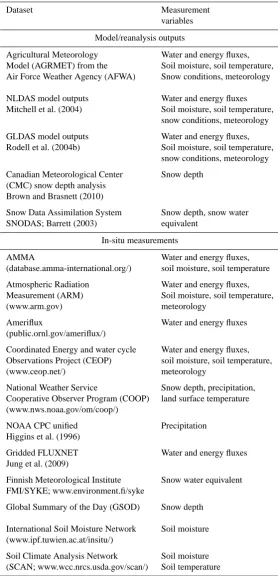
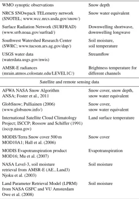
The key processes that constitute the terrestrial hydrological cycle include precipitation, radiation, interception of precip-itation by vegetation, infiltration of precipprecip-itation into the soil and the vertical transfer of soil moisture, evapotranspiration, formation of snow, snow melt, and river runoffs, among oth-ers. In order to quantify the contribution of these individual processes to the overall variability of the terrestrial hydro-logical cycle, they must be evaluated against the full suite of available measurements. Motivated by this goal, the pro-cessing of a large set of measurements of different processes from a variety of sources are supported in LVT. As shown in Table 1, these datasets constitute the monitoring of different components of the terrestrial hydrological cycle, from differ-ent observing platforms. The spatial and temporal scales of these measurements also vary significantly. By incorporat-ing the processincorporat-ing of these datasets under a sincorporat-ingle, integrated framework, LVT enables an environment for performing a comprehensive evaluation of the terrestrial hydrological pro-cesses. Note that the support of this large suite of products is enabled by the extensible nature of LVT software design and is expected to further expedite the incorporation of other relevant datasets in the future.
4.2 Analysis metrics
Table 1. List of datasets supported in LVT.
Dataset Measurement
variables
Model/reanalysis outputs
Agricultural Meteorology Water and energy fluxes,
Model (AGRMET) from the Soil moisture, soil temperature,
Air Force Weather Agency (AFWA) Snow conditions, meteorology
NLDAS model outputs Water and energy fluxes
Mitchell et al. (2004) Soil moisture, soil temperature,
snow conditions, meteorology
GLDAS model outputs Water and energy fluxes,
Rodell et al. (2004b) Soil moisture, soil temperature,
snow conditions, meteorology
Canadian Meteorological Center Snow depth
(CMC) snow depth analysis Brown and Brasnett (2010)
Snow Data Assimilation System Snow depth, snow water
SNODAS; Barrett (2003) equivalent
In-situ measurements
AMMA Water and energy fluxes,
(database.amma-international.org/) soil moisture, soil temperature
Atmospheric Radiation Water and energy fluxes,
Measurement (ARM) Soil moisture, soil temperature,
(www.arm.gov) meteorology
Ameriflux Water and energy fluxes
(public.ornl.gov/ameriflux/)
Coordinated Energy and water cycle Water and energy fluxes, Observations Project (CEOP) soil moisture, soil temperature,
(www.ceop.net/) meteorology
National Weather Service Snow depth, precipitation,
Cooperative Observer Program (COOP) land surface temperature (www.nws.noaa.gov/om/coop/)
NOAA CPC unified Precipitation
Higgins et al. (1996)
Gridded FLUXNET Water and energy fluxes
Jung et al. (2009)
Finnish Meteorological Institute Snow water equivalent FMI/SYKE; www.environment.fi/syke
Global Summary of the Day (GSOD) Snow depth
International Soil Moisture Network Soil moisture (www.ipf.tuwien.ac.at/insitu/)
Soil Climate Analysis Network Soil moisture
Table 1. Continued.
WMO synoptic observations Snow depth
NRCS SNOwpack TELemetry network Snow water equivalent
(SNOTEL; www.wcc.nrcs.usda.gov/snow/)
Surface Radiation Network (SURFRAD) Downwelling shortwave,
(www.srrb.noaa.gov/surfrad/) downwelling longwave
Southwest Watershed Research Center Soil moisture,
(SWRC; www.tucson.ars.ag.gov/dap/) soil temperature
USGS water data Streamflow
(waterdata.usgs.gov/nwis)
AMSR-E radiances Brightness temperature for
(mrain.atmos.colostate.edu/LEVEL1C/) different channels
Satellite and remote sensing data
AFWA NASA Snow Algorithm Snow cover, snow depth,
ANSA; Foster et al., 2011 snow water equivalent
GlobSnow; Pulliainen (2006) Snow cover,
(www.globsnow.info/) snow water equivalent
International Satellite Cloud Climatology Land surface temperature Project; ISCCP; Rossow and Schiffer (1991)
(isccp.nasa.gov)
MODIS/Terra Snow cover 500 m Snow cover
MOD10A1; Hall et al. (2006)
MODIS Evapotranspiration product Evapotranspiration
MOD16; Mu et al. (2007)
NASA Level-3, soil moisture Soil moisture
retrieval from AMSR-E (AE−Land3) Njoku et al. (2003)
Land Parameter Retrieval Model (LPRM) Soil moisture from NASA GSFC and VU Amsterdam
Owe et al. (2008)
may also differ significantly based on the targeted applica-tion (Gupta et al., 2009). Model evaluaapplica-tion studies quite of-ten use accuracy-based metrics that quantify model perfor-mance using residual-based measures. These metrics, how-ever, may not provide further insights on the robustness of the model under future or unobserved scenarios (Pachepsky et al., 2006). They are also inadequate in capturing estimates of associated uncertainties (Gulden et al., 2008), relative im-portance and sensitivity of model parameters to the overall accuracy and uncertainty, tradeoffs in performance due to spatial scales and the tradeoffs between actual information content and variabilities introduced by random noise. Gupta et al. (2008) emphasize the need for sophisticated diagnostic evaluation methods that help in isolating the limitations of the model representations.
A number of analysis metric types is supported in LVT including (1) statistical accuracy measures that are
of metrics enables novel ways to quantify and translate model performance.
4.3 Miscellaneous features
LVT also supports a number of miscellaneous features to as-sist the verification procedures. To provide a measure of the statistical significance and the influence of sampling density on the results, confidence intervals based on Gaussian distri-butions are computed for each verification metric. Note that LVT does not include any graphical packages in it. LVT gen-erates the results of the analyses in ASCII text, binary, GriB and NetCDF output formats and the generation of appropri-ate graphics are left to the user. The capabilities to generappropri-ate probability density functions (PDFs) of the computed met-rics by stratifying to specified parameters are also included in LVT. Further, LVT also provides methods to impose user-defined masking to exclude selected grid points when anal-ysis metrics are computed. These masks can be static, time-varying or based on a certain variable. For example, a down-ward shortwave radiation (SW↓) based mask can be defined that separates the analysis computations when the SW↓ val-ues are above and below a specified threshold (say 5 W m−2). This will enable a day-night stratification of the computed metrics, when SW↓ values are above and below 5 W m−2, respectively.
LVT also includes a number of land surface process di-agnostics related to the partitioning of energy across the land atmosphere interface, such as evaporative fraction, bowen ra-tio and overall energy, water and evaporara-tion budgets at the land-atmosphere interface. These diagnostics are computed for both model and observational datasets. Quantifying these diagnostics are important for improving the understanding of the feedbacks between the land surface and the atmosphere.
As mentioned earlier, LVT also supports the analysis of diagnostics generated by the LIS data assimilation subsys-tem. These include distribution statistics of data assimilation innovations and analysis gain, which provide measures of the efficiency of data assimilation configurations. Similarly, LVT also handles the outputs of the optimization and uncer-tainty estimation subsystems of LIS. For example, checks to assess the convergence of these iterative algorithms can be performed by analyzing the optimization and uncertainty es-timation outputs through LVT.
In the examples presented in Sect. 5, LVT is employed in serial mode, as the support of computational parallelism is currently under development. The memory and CPU require-ments and the corresponding computational performance of LVT are largely determined by the analysis domain, the datasets being used and the metrics being computed.
Though LVT was originally designed to support LIS out-puts, it has since been extended to facilitate the evaluation of other “non-LIS” model products. LVT contains the features to convert the given non-LIS product to a LIS output style and format. It then uses the converted output for evaluation.
0 50 100 150 200 250 300
0 5 10 15 20 25
Latent Heat Flux (W/m2)
Hour DEFAULT CALIBRATED OBS
-100 -50 0 50 100 150 200 250 300 350
0 5 10 15 20 25
Sensible Heat Flux (W/m2)
Hour DEFAULT CALIBRATED OBS
Fig. 3.Comparison of average diurnal cycles of latent (left column) and sensible heat (right column) fluxes from the uncoupled Noah (version 3.2) LSM simulations using the default model parameters (DEFAULT) and calibrated parameters (CALIBRATED) against the in-situ measurements (OBS) from 19 ARM-SGP stations.
28
Fig. 3. Comparison of average diurnal cycles of latent (left column) and sensible heat (right column) fluxes from the uncoupled Noah (version 3.2) LSM simulations using the default model parameters (DEFAULT) and calibrated parameters (CALIBRATED) against the in-situ measurements (OBS) from 19 ARM-SGP stations.
Note that this process does not involve any spatial or tem-poral transformation of the data, rather the conversion to a different data format and convention.
5 Model evaluation examples using LVT
5.1 An end-to-end example of the MDF paradigm
As noted earlier, one of the key motivations behind LVT is to provide a system that can augment LIS’ modeling capabili-ties with an evaluation framework. The joint use of both these systems enables an end-to-end environment for facilitating the steps of the MDF paradigm. In this section, we present an example of using the modeling and computational tools in LIS to refine the model performance and the verification features in LVT to quantitatively evaluate the simulations.
Model simulations using the Noah LSM (version 3.2) (Ek et al., 2003; Barlage et al., 2010) forced with the NLDAS-II datasets are conducted over a 500×500 domain covering the US Southern Great Plains (SGP) at 1 km spatial resolution during the time period of 1 May 2006 to 1 September 2006. This domain is used in a number of prior studies on land-atmosphere feedbacks (Santanello et al., 2009, 2011). Using the default values of the soil and vegetation parameters of the Noah LSM, a model simulation is conducted first to simulate surface latent and sensible heat flux estimates. Using LVT, these flux estimates are evaluated against the in-situ measure-ments from 19 Atmospheric Radiation Measurement (ARM) stations. The optimization algorithms in LIS are then used to estimate a refined set of model parameters with the objective of minimizing the cumulative error in the hourly surface flux observations from the ARM stations, over the four month period. The optimization simulations were used to estimate 29 model parameters in the Noah LSM that included both soil and vegetation properties. Subsequently, the improved model performance with the calibrated parameters is quanti-fied using LVT.
Table 2. The range of analysis metric types and implementations supported in LVT.
Metric class Supported
Implementations
Standard measures RMSE, Anomaly RMSE, unbiased RMSE (ubRMSE), Correlation, Anomaly correlation, Mean absolute error (MAE), Bias, Probability of “yes” detection (PODy), False alarm ratio (FAR) Probability of “no” detection (PODn), Accuracy measure (ACC), Probability of false detection (POFD), Critical success index (CSI), Equitable threat score (ETS), Frequency bias (FBIAS),
Nash sutcliffe efficiency (NSE)
Ensemble metrics Mean, Standard deviation, Likelihood
Uncertainty metrics Uncertainty importance
Information theoretic Metric entropy, Information gain, Effective complexity, Fluctuation complexity
Data assimilation metrics Mean, variance, lag correlation of innovation distributions
Spatial similarity metrics Spatial area, Hausdorff distance
Scale decomposition Discrete wavelet transforms
stations. The simulations using default model parameters show large errors, with a significant underestimation in the latent heat fluxes and an overestimation in sensible heat fluxes. The calibration of model parameters helps in improv-ing the model performance, by correctimprov-ing the systematic bias in energy partitioning. This example illustrates an example of the MDF paradigm that includes model characterization, reformulation through parameter estimation, and verification using LVT. Similar instances can be implemented using the extensive evaluation capabilities of LVT.
5.2 Example of model evaluation against satellite data
Model formulation and evaluation are typically conducted over instrumented locations of the world where indepen-dent measurements are available. Though these in-situ ob-servations provide valuable information on the spatial and temporal variability of process variables, they are limited in their spatial coverage. Satellite and remotely-sensed mea-surements, on the other hand, have improved spatial cov-erages and they enable the extension of model evaluation to uninstrumented locations and hydrologic regimes. In this section, we present an example of model evaluation against satellite data over a region where in-situ measurements are sparse.
A model simulation using Noah LSM (version 2.7.1) is conducted over a 1200 km×1000 km domain, at 1 km spa-tial resolution over Afghanistan from 1 October 2007 to 1 May 2010. The LSM is driven with meteorological data from the Global Data Assimilation System (GDAS); the global meteorological weather forecast model of the National Centers for Environmental Prediction (Derber et al., 1991). The precipitation input for the model simulations is pro-vided from the NOAA Climate Prediction Center’s (CPC) operational global 2.5◦5-day Merged Analysis of Precipita-tion (CMAP; Xie and Arkin, 1997), which is a product that
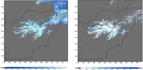
Fig. 4.Probability of Detection (left column) and False Alarm Ratio (right column) of the model simulated snow cover fields compared against the fractional MODIS snow cover product (MOD10A1).
29
Fig. 4. Probability of Detection (left column) and False Alarm Ratio (right column) of the model simulated snow cover fields compared against the fractional MODIS snow cover product (MOD10A1).
employs blended satellite (IR and microwave) and gauge ob-servations. The model domain has complex terrain character-istics, with elevation ranges from 1000 to 6000 m. The frac-tional snow cover extent global 500 m product (MOD10A1 Version 4; Hall et al., 2006) from the Moderate Resolution Imaging Spectroradiometer (MODIS) optical sensor on the Terra spacecraft is used as the reference data for evaluating simulations of snow cover fields simulated by the LSM. The MOD10A1 product is aggregated to 1 km spatial resolution for enabling the comparisons presented here.
FAR fields display the terrain features of the Hindu Kush mountains, that run northeast to southwest. High values of POD and low values of FAR are observed over the Central Highlands region of the domain, suggesting a high degree of accuracy of model snow cover estimates over these areas. Over the northeast parts of the domain, however, the model simulations are less accurate, as indicated by the lower POD and higher FAR values.
5.3 Analysis of data assimilation diagnostics
The example in Sect. 5.1 presents an instance of the MDF paradigm that employs parameter estimation for model re-formulation. As noted in Williams et al. (2009), similar MDF instances can be defined that employ data assimilation tech-niques to improve state estimation. This section presents an example of using data assimilation diagnostics to assess the performance of the system within a MDF context.
The difference between the observations being assimilated and the model forecasts, known as innovations, are typically computed during data assimilation. The statistics of the in-novations are typically used to diagnose the performance of the assimilation algorithm. For example, when the Ensemble Kalman Filter (EnKF) is used as the assimilation algorithm, a linear system dynamics is assumed with Gaussian, mutually and serially uncorrelated errors in model and observations (Reichle and Koster, 2002). Consequently, the distribution of normalized innovations (normalized with their expected co-variance) is expected to follow a standard normal distribution
N (0,1)(Gelb, 1974). The deviations from the expected mean and standard deviation of the normalized innovation distribu-tion is used as a measure of suboptimality of the data assimi-lation configuration. A number of studies have confirmed that poor specification of model and observation error parameters can significantly degrade the quality of assimilation products (Reichle and Crow, 2008; Reichle et al., 2008). The assimi-lation diagnostics can be analyzed using LVT and the model and observation error specifications can then be continually revised to ensure optimal data assimilation performance.
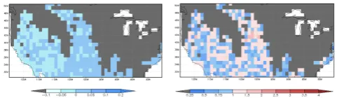
To demonstrate these capabilities, a synthetic data assim-ilation experiment is conducted over the Continental US do-main at 1◦ spatial resolution, for a time period of 1 Jan-uary 2000 to 1 JanJan-uary 2006. In this experiment, the obser-vations to be assimilated are synthetically simulated (from an independent land model simulation using the Catchment LSM) and as a result, the associated errors are perfectly known. The observations are assimilated using the Ensemble Kalman Filter (EnKF) algorithm. The details of the assim-ilation setup are provided in Kumar et al. (2012). Figure 5 shows the spatial distribution of mean and variance of nor-malized innovations over the domain generated by the assim-ilation system. In this instance, the mean values are close to zero and the variances are closer to 1, indicating near-optimal performance. Additional analysis metrics, such as lag corre-lation coefficients to assess the “whiteness” of the innovation
Fig. 5.Mean (left column) and variance (right column) of normalized innovations (dimensionless) of data assimilation diagnostics. The gray color represents grid cells excluded from the computations.
30
Fig. 5. Mean (left column) and variance (right column) of normal-ized innovations (dimensionless) of data assimilation diagnostics. The gray color represents grid cells excluded from the computa-tions.
distribution, are also provided within LVT for more detailed evaluations of the efficiency of the data assimilation system.
5.4 Characterization of uncertainty diagnostics
It is well acknowledged that model simulations and observa-tions are affected by different sources of uncertainties. The errors in model parameters, input forcing and structural de-ficiencies introduce uncertainties in the model simulations. The measurements from satellite and remote sensing plat-forms are subject to measurement noise and errors in retrieval models. Similarly, the in-situ measurements also have asso-ciated uncertainties due to environmental factors, data pro-cessing and instrument errors. Therefore, it is important to quantify the impact of these uncertainty sources in modeled estimates. LVT includes a number of measures to quantify the propagation of model parameter uncertainty in predic-tions.
(a)
0 0.1 0.2 0.3 0.4 0.5
2010/05 2010/06 2010/07 2010/08 2010/09
Soil Moisture (m3/m3)
Ensemble Mean Obs
(b)
0 0.5 1 1.5
2010/05 2010/06 2010/07 2010/08 2010/09
Uncertainty Importance (-)
θs Ψs
Ks
b
Fig. 6.(a) Comparison of ensemble soil moisture simulations against observations. The cyan shading indicates the ensemble spread, shown as±2×ensemble standard deviation (b) The uncertainty importance of model parameters towards soil moisture uncertainty.
31
Fig. 6. (a) Comparison of ensemble soil moisture simulations against observations. The cyan shading indicates the ensemble spread, shown as±2×ensemble standard deviation. (b) The tainty importance of model parameters towards soil moisture uncer-tainty.
as±2×the ensemble standard deviation) around the ensem-ble mean represents the uncertainty in simulated soil mois-ture. The soil moisture uncertainty is small during the dry pe-riod, but grows significantly during the late summer months when both the magnitude and variability of soil moisture in-crease. Though the spread of the ensemble encompasses the observations, the observations tend to fall towards the tail end of the ensemble distribution. This emphasizes the need to re-fine the model parameters and their sampling strategies for a better characterization of modeling uncertainty.
Figure 6b also provides an uncertainty importance mea-sure which is an assessment of the relative contribution of each parameter to the ensemble spread. This metric is com-puted as the correlation between the simulated variable (sur-face soil moisture) and the parameter across the ensemble. Figure 6b suggests that among the four SHPs considered, model simulations are most sensitive toθs, followed byKs. The variability inψsand thebparameters contribute less to the uncertainty in soil moisture in this instance. The figure also illustrates that the relative importance of the parameter is
sensitive to the soil moisture magnitude and variability. Dur-ing the late summer months, the uncertainty importance ofθs also increases with the magnitude of simulated soil moisture. Knowledge of the relative importance of the model parame-ters is significant when choosing the set of model parameparame-ters for calibration and sampling, and LVT facilitates the quantifi-cation of such sensitivities. Similar to the examples described in Sects. 5.1 and 5.3, this example provides another instance of using LVT to enable the MDF concept, in the context of uncertainty estimation.
5.5 Information theory metrics
A number of studies (Wackerbauer et al., 1994; Lange, 1999) describe the use of information theory-based metrics to dis-criminate time series data based on their information con-tent (or randomness) and their complexity. Pachepsky et al. (2006) and Pan et al. (2011) describe the use of these mea-sures for discriminating soil water models. LVT includes a number of information theory-based measures such as met-ric entropy, mean information gain, effective complexity and fluctuation complexity. These measures are computed by converting the time series of a given dataset into a binary symbol string (Lange, 1999). Within the symbol string, pat-terns of words (defined as a group of consecutive symbols of a certain length) are identified, representing a state of the system of interest. For example, a word consisting ofL con-secutive symbols has 2Lpossible states. The information the-ory metrics are then defined by computing the probabilities associated with the patterns of words in the converted time series of the data. For example, the metric entropy (ME) and information gain (IG) metrics are defined as follows:
ME= −1 L
2L X
i=1
pilog2pi (1)
IG= − 2L X
i,j=1
pL,ijlog2pL,i→j, (2)
wherepi is the probability of occurrence of thei-th word,
pL,ij is the probability of transition from thei-th to thej-th word, andpL,i→jis the conditional probability of the occur-rence of thej-th word given that thei-th word has already oc-curred in the symbol sequence. A more detailed description of these measures are provided in Pachepsky et al. (2006).
The information theory-based metrics are typically ap-plied to discriminate model simulations, especially when they yield similar accuracy measures. Here we demonstrate their use for comparing soil moisture simulations from Noah LSM (version 3.2) when two different retrievals from the Ad-vanced Microwave Scanning Radiometer for the Earth Ob-serving System (AMSR-E) sensor aboard the Aqua satellite are assimilated. The NASA Level-3, “AE−Land3” product
Fig. 7.Changes in Metric Entropy (top row) and Information gain (bottom row) from the assimilation of NASA
AMSR-E (left column) and LPRM AMSR-E (right column) retrievals
32
Fig. 7. Changes in Metric Entropy (top row) and Information gain (bottom row) from the assimilation of NASA AMSR-E (left column) and LPRM AMSR-E (right column) retrievals.
GSFC and VU Amsterdam (Owe et al., 2008) are used in the data assimilation (DA) integrations. The experiments are carried out over the Continental United States for a period of 2002 to 2008, using the same configuration used in the NLDAS project (Mitchell et al., 2004) (from 25–53◦N and
125–67◦W at 1/8 degree spatial resolution). The details of
the assimilation methodology are described in Peters-Lidard et al. (2011).
Figure 7 presents a comparison of the change in metric entropy (1ME) and the information gain (1IG) metric as a result of data assimilation. These metric values are com-puted using a word length of 3. The 1ME and 1IG val-ues are calculated by subtracting the metric valval-ues for the simulation without data assimilation from the corresponding data assimilation integration. Figure 7 indicates that DA in-troduces more entropy (randomness) in the simulations, over most parts of the domain, with higher values of 1ME for the NASA DA compared to the LPRM DA. The information gain metric indicates how much the sequence of patterns in the data contributes to the overall information. The1IG val-ues when assimilating NASA retrievals are larger compared to that of LPRM assimilation. The changes in soil moisture introduced by the NASA DA also result in more randomness
in the consecutive patterns in the time series. This leads to higher IG values for NASA DA relative to LPRM DA, sug-gesting that the changes in soil moisture time series intro-duced by LPRM DA may be less spurious (random). In prior MDF studies (Reichle et al., 2007; Q. Liu et al., 2011; Peters-Lidard et al., 2011), accuracy-based measures were used to characterize the value of assimilating these retrievals into LSMs. The results in this article present an alternate eval-uation using information theory metrics within LVT.
5.6 Scale decomposition features
0 5 10 15 20 25 30 35
1 2 4 8 16 32 64 128 256 512 1024
Percentage contribution
Spatial Scale (KM)
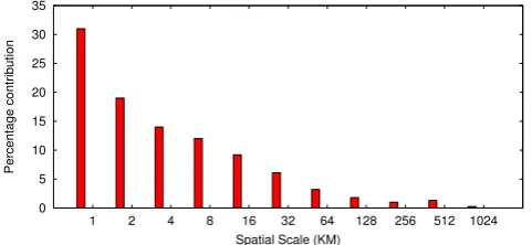
Fig. 8.Percentage contribution to the total improvement in snow covered area POD at different spatial scales, generated by a two dimensional discrete Haar wavelet analysis.
33
Fig. 8. Percentage contribution to the total improvement in snow covered area POD at different spatial scales, generated by a two dimensional discrete Haar wavelet analysis.
an example of scale-decomposition evaluation of snow cover simulations from the LSMs using LVT.
The intensity-scale approach of Casati et al. (2004), orig-inally developed for the spatial verification of precipitation forecasts, is used to perform a scale decomposition analy-sis. The technique employs a two dimensional discrete Haar wavelet transform that decomposes a given field into the sum of orthogonal components at different spatial scales. The mean squared error (MSE) of the decomposed components at each spatial scale is used to quantify the scale decomposition effects.
Using the domain configuration at 1 km spatial resolution over Afghanistan (used in Sect. 5.1), two model simulations are conducted using Noah LSM (version 2.7.1); one that em-ploys a terrain based correction of shortwave radiation input to the LSM and one that does not include such adjustments. The terrain-based corrections adjust the incoming shortwave radiation based on terrain slope and aspect, and these changes in turn impact the evolution of snow over these terrain. The improvements in the snow cover simulation as a result of the terrain-based correction is computed as the difference in POD fields from the two simulations, generated by compar-ing against the MOD10A1 (version 4) fractional snow cover product. The scale-decomposition approach is then applied to this difference field, to quantify how the improvements in snow cover estimates at 1 km spatial resolution translate to coarser spatial scales.
Figure 8 shows the result of scale decomposition of the to-tal improvement field for POD using the two dimensional discrete Haar wavelet transform. The algorithm computes successive decompositions of the original field by powers of 2. The percentage contribution to the total improvement at each coarse spatial scale is shown in Fig. 8. The results indi-cate that most of the improvements in POD are obtained at fine spatial scales and the contribution of the scale decreases with increase in spatial resolution. At scales coarser than 16 km, the percentage contribution drops below 10 %. Simi-lar analysis of scale effects can be performed on other metrics and variables of interest. This example demonstrates the use
of LVT for another MDF experiment where the MODIS frac-tional snow cover data is used to assess the applicability of model formulations at different spatial scales.
5.7 Spatial similarity measures
With the increased availability of spatially distributed datasets from satellites and remote-sensing platforms, there is a need for techniques and metrics that evaluate models and observations based on the their spatial patterns, in addi-tion to the one-to-one correspondence comparisons that are typically used. The incorporation of spatial pattern compar-isons will aid in further improving the reliability of LSMs for hydrological applications (Bloschl and Sivapalan, 1995; Grayson and Bloschl, 2000). A review of spatial similarity methods in hydrology is provided in Wealands et al. (2005), which includes techniques based on statistical identification as well as image processing techniques. In this section, an ex-ample of using a similarity metric through LVT to compare snow cover patterns from two different LSMs is presented.
Snow cover estimates using two LSMs, Noah (version 3.2) and CLM (version 2; Dai et al., 2003), forced with GDAS and CMAP datasets, are generated over a 100×100 region near the Southern Great Plains in the US at 1 km spatial resolution for a time period of 1 November 2008 to 1 June 2009. The LSMs have different representations of snow processes, with Noah employing a simple single snow layer scheme. CLM includes a more complex five layer snow scheme with param-eterizations for temporally varying snow albedo, as a func-tion of snow cover and snow age. Both LSMs simulate tem-porally varying snow density with evolution of patchy snow cover. The model simulations are evaluated against the frac-tional snow cover observations from MODIS (MOD10A1 version 4) using the “Hausdorff distance” similarity metric.
Hausdorff distance (HD) measures the similarity of points in two finite sets and is not designed to find one-to-one cor-respondence between points in each set. It is expressed as the maximum distance of a set to the nearest point in the other set:
h(M, O)=max m∈M
{min
o∈O
{||m−o||}}, (3)
whereh(M, O)is the HD value,mandoare points of sets
M(representing model) andO (representing observations), respectively.||m−o||is the norm of the points in the model and observation spaces and can be computed as the Euclidean distance betweenmando.
0 1 2 3 4 5 6 7 8
2008/11 2009/01 2009/03 2009/05
Hausdorff distance
Noah CLM
Fig. 9.Comparison of the cumulative Hausdorff distance measures of snow cover simulations from Noah and CLM
34
Fig. 9. Comparison of the cumulative Hausdorff distance measures of snow cover simulations from Noah and CLM.
patterns during the peak snow season. During the snow melt period, Noah produces lower HD values compared to CLM. This suggests that the spatial patterns in the Noah snow cover simulations capture the observational patterns more accu-rately relative to CLM’s simulations, though CLM’s snow physics formulations are more complex. Note that newer ver-sions of both these models (Noah-MP; Niu et al., 2011) and CLM version 4.0 (Lawrence et al., 2011) with updated snow physics formulations are currently being incorporated into LIS, and similar comparisons can be performed through LVT to evaluate the updated snow physics in these LSMs. This experiment demonstrates the use of spatial similarity metrics for comparing the performance of two different LSMs within a MDF framework.
6 Summary and future directions
This article describes the development and capabilities of a verification system for terrestrial hydrology known as the Land surface Verification Toolkit. LVT enables an environ-ment for conducting the systematic evaluation of land model outputs by providing a variety of analysis metrics and proce-dures. LVT functions primarily as an analysis back-end sys-tem for the NASA Land Information Syssys-tem (LIS), but also supports the analysis of data products from other modeling environments. LIS is a comprehensive land surface modeling framework and includes data assimilation and posterior infer-ence tools such as optimization and uncertainty estimation to facilitate the exploitation of information content from ob-servational datasets to augment model predictions. LVT not only supports the verification of LSM outputs, but also pro-vides the tools to analyze the performance of these computa-tional algorithms within LIS. LVT is designed using object oriented software principles, with abstractions defined for the customization and extension of the system for different
applications. These extensible interfaces allow the incorpo-ration of new observational datasets and analysis metrics in an interoperable manner. The combination of the modeling capabilities of LIS and the analysis capabilities of LVT pro-vide a robust environment for conducting end-to-end model data fusion experiments that has been identified in the com-munity as a key paradigm for improving the applicability of LSMs.
LVT currently supports a large suite of in-situ, satellite and remotely-sensed, and model and reanalysis products to enable comprehensive evaluations of various hydrological processes. These datasets are supported in their native for-mat and LVT handles the temporal and spatial transforma-tions required in the analysis. Diagnostic model verifica-tion and intercomparisons are supported through a variety of analysis metrics and procedures. In addition to the stan-dard accuracy-based measures, LVT supports ensemble and uncertainty measures, metrics based on information theory, similarity metrics and methods to quantify the impact of spa-tial scales on model performance. This variety of techniques provide novel ways to characterize model performance and to investigate associated tradeoffs.
The article presents a number of illustrative examples that demonstrate the capabilities of LVT and provide several in-stances of end-to-end MDF experiments. The optimization algorithms in LIS are used to refine the model parameters of the LSM to improve its estimation of surface fluxes. LVT is used to quantify the systematic improvements resulting from the refined model parameters. The impact of data fusion for model state and uncertainty estimation is assessed through data assimilation and uncertainty quantification metrics, re-spectively. The information theory-based metrics provide measures such as metric entropy, information gain and com-plexity to identify tradeoffs in datasets based on their infor-mation content and complexity. Acknowledging the need to perform model evaluations in a spatially distributed manner, spatial similarity metrics and scale decomposition techniques that provide spatial pattern comparisons against remotely-sensed distributed datasets are also incorporated in LVT.
of drought (Heim, 2002). The availability of these drought indices through LVT will enable cross-comparisons of these measures and the assessment of their suitability for the in-tended application. In summary, the growing capabilities of LVT are expected to help in the definition and refinement of a formal benchmarking and evaluation process for the LSMs and assist in improving their use for real-world applications.
Acknowledgements. We gratefully acknowledge the financial
support from NASA Earth Science Technology Office (ESTO) and the US Air Force Weather Agency (AFWA) and the assis-tance from summer intern students Teodor Georgiev (Princeton University), Yi Yuan (University of Michigan) and Corina Robles (Florida International University) for assembling evaluation datasets and the software testing of LVT. Computing was sup-ported by the resources at the NASA Center for Climate Simulation.
Edited by: D. Lawrence
References
Abramowitz, G., Leuning, R., Clark, M., and Pitman, A.: Evaluating the performance of land surface models, J. Climate, 21, 5468– 5481, 2008.
Barlage, M., Chen, F., Tewari, M., Ikeda, K., Gochis, D., Dudhia, J., Rasmussen, R., Livneh, B., Ek, M., and Mitchell, M.: Noah Land Surface Model modifications to improve snowpack prediction in the Colorado Rocky Mountains, J. Geophys. Res., 115, D22101, doi:10.1029/2009JD013470, 2010.
Barrett, A.: National Operational Hydrologic Remote Sensing Cen-ter Snow Data Assimilation System (SNODAS) products at NSIDC, Tech. rep., National Snow and Ice Data Center, Boul-der, CO, digital Media, 2003.
Bloschl, G.: Scaling issues in snow hydrology, Hydrol. Process., 13, 2149–2175, 1999.
Bl¨oschl, G. and Sivapalan, M.: Scale issues in hydrological model-ing, Hydrol. Process., 9, 251–290, 1995.
Blyth, E., Gash, J., Lloyd, A., Pryor, M., Weedon, G., and Shuttle-worth, J.: Evaluating the JULES model energy fluxes using the FLUXNET data, J. Hydrometeor., 11, 509–519, 2010.
Blyth, E., Clark, D. B., Ellis, R., Huntingford, C., Los, S., Pryor, M., Best, M., and Sitch, S.: A comprehensive set of benchmark tests for a land surface model of simultaneous fluxes of water and carbon at both the global and seasonal scale, Geosci. Model Dev., 4, 255–269, doi:10.5194/gmd-4-255-2011, 2011.
Brown, R. and Brasnett, B.: Canadian Meteorological Center (CMC) daily snow analysis data, Tech. rep., National Snow and Ice Data Center, Boulder, CO, digital Media, 2010.
Brown, B., Gotway, J., Bullock, R., Gilleland, E., Fowler, T., Ahi-jevych, D., and Jensen, T.: The Model Evaluation Tools (MET): Community tools for forecast evaluation, in: 25th Conf. on Inter-national Interactive Information and Processing Systems (IIPS) for Meteorology, Oceanography, and Hydrology, Amer. Metero. Soc., Phoenix, AZ, 2009.
Brown, J., Demargne, J., Seo, D.-J., and Liu, Y.: The Ensemble Ver-ification System (EVS): a software tool for verifying ensemble foreasts of hydrometeorological and hydrologic variables at dis-crete locations, Environ. Model. Software, 25, 854–872, 2010.
Casati, B., Ross, G., and Stephenson, D. B.: A new intensity- scale approach for the verification of spatial precipitation forecasts, Meteor. Appl., 11, 141–154, 2004.
Chen, F., Mitchell, K., Schaake, J., Xue, Y., Pan, H., Koren, V., Duan, Y., Ek, M., and Betts, A.: Modeling of land-surface evapo-ration by four schemes and comparison with FIFE observations, J. Geophys. Res., 101, 7251–7268, 1996.
Dai, Y., Zeng, X., Dickinson, R., Baker, I., Bonan, G., Bosilovich, M., Denning, S., Dirmeyer, P., Houser, P., Niu, G., Oleson, K., Schlosser, A., and Yang, Z.-L.: The common land model (CLM), B. Am. Meteorol. Soc., 84, 1013–1023, doi:10.1175/BAMS-84-8-1013, 2003.
Decyk, V. K., Norton, C. D., and Szymanski, B. K.: How to ex-press C++ concepts in Fortran 90, Scientific Programming, 6, 363–390, 1997.
Derber, J., Parrish, D., and Lord, S.: The new global operational analysis system at the National Meteorological Center, Weather Forecast., 6, 538–547, 1991.
de Rosnay, P., Boone, A., Beljaars, A., and Polcher, J.: AMMA Land surface intercomparison projects, GEWEX News, 16, 10– 11, 2006.
Dirmeyer, P., Gao, X., Zhao, M., Guo, Z., Oki, T., and Hanasaki, N.: GSWP-2: Multimodel analysis and implications for our percep-tion of the land surface, B. Am. Meteorol. Soc., 87, 1381–1397, doi:10.1175/BAMS-87-10-1381, 2006.
Ek, M. B., Mitchell, K. E., Lin, Y., Rogers, E., Grunmann, P., Ko-ren, V., Gayno, G., and Tarpley, J. D.: Implementation of Noah land surface model advances in the National Centers for Environ-mental Prediction operational mesoscale Eta model, J. Geophys. Res., 108, 8851, doi:10.1029/2002JD003296, 2003.
Entekhabi, D., Asrar, G., Betts, A., Beven, K., Bras, R., Duffy, C., Dunne, T., Koster, R., Lettenmaier, D., McLaughlin, D., Shut-tleworth, W., van Genuchten, M., Wei, M.-Y., and Wood, E.: An agenda for land surface hydrology research and a call for the sec-ond international hydrological decade, B. Am. Meteorol. Soc., 80, 2043–2058, 1999.
Entekhabi, D., Reichle, R., Koster, R., and Crow, W.: Per-formance Metrics for Soil Moisture Retrievals and Ap-plication Requirements, J. Hydrometeor., 11, 832–840, doi:10.1175/2010JHM1223.1, 2010.
Erickson, T. A., Williams, M. W., and Winstral, A.: Persistence of topographic controls on the spatial distribution of snow in rugged mountain terrain, Colorado, United States, Water Resour. Res., 41, W04014, doi:10.1029/2003WR002973, 2005.
Fennessey, M. and Shukla, J.: Impact of initial soil wetness on sea-sonal atmospheric prediction, J. Climate, 12, 3167–3180, 1999. Foster, J., Hall, D., Eylander, J., Riggs, G., Nghiem, S., Tedesco,
M., Kim, E., Montesano, P., Kelly, R., Casey, K. A., and Choud-hury, B.: A blended global snow product using visible, passive microwave and scatterometer satellite data, Int. J. Remote Sens., 32, 5, doi:10.1080/01431160903548013, 2011.
Friend, A. and Kiang, N.: Land surface model development for the GISS GCM: Effects of improved canopy physiology on simu-lated climate, J. Climate, 18, 2883–2902, 2005.
Gelb, A.: Applied Optimal Estimation, MIT Press, Cambridge, MA, 1974.
Gulden, L., Rosero, E., Yang, Z.-L., Wagener, T., and Niu, G.-Y.: Model performance, model robustness, and model fitness scores: A new method for identifying good land surface models, Geo-phys. Res. Lett., 35, L11404, doi:10.1029/2008GL033721, 2008. Gupta, V., Rodriguez-Iturbe, I., and Wood, E.: Scale problems in
Hydrology, Reidel, Dordrecht, 1986.
Gupta, H., Wagener, T., and Liu, Y.: Reconciling theory with obser-vations: elements of a diagnostic approach to model evaluation, Hydrol. Process., 22, 3802–3813, doi:10.1002/hyp.6989, 2008. Gupta, H., Kling, H., Yilmaz, K., and Martinez, G.: Decomposition
of the mean squared error and NSE performance criteria: Im-plications for improving hydrological modeling, J. Hydrol., 377, 80–91, doi:10.1016/j.jhydrol.2009.08.003, 2009.
Hall, D., Riggs, G., and Salomonson, V.: MODIS/Terra snow cover daily L3 Global 500 m Grid V005, Tech. rep., National Snow and Ice Data Center, Colorado, USA, digital media, 2006.
Harrison, K., Kumar, S., Peters-Lidard, C., and Santanello, J.: Quantifying soil moisture modeling uncertainty with remote sensing observations using Bayesian inference techniques, Wa-ter Resour. Res., under review, 2012.
Heim, R. J.: A review of twentieth century drought indices used in the United States, B. Am. Meteorol. Soc., 83, 1149–1165, 2002. Henderson-Sellers, A., Pitman, A., Love, P., Irannejad, P., and Chen, T.: The project for Intercomparison of land surface parameteri-zation schemes (PILPS): Phases 2 and 3, B. Am. Meteorol. Soc., 76, 489–503, 1995.
Higgins, R., Janowiak, J., and Yao, Y.-P.: A gridded hourly precip-itation database for the United States (1963–1993)., Tech. rep., NCEP Climate Prediction Center Atlas 1, 46 pp., 1996. Hill, C., DeLuca, C., Balaji, V., Suarez, M., and da Silva, A.: The
Architecture of the Earth System Modeling Framework, Comput. Sci. Eng., 6, 18–28, 2004.
Jiminez, C., Prigent, C., Mueller, B., Seneviratne, S., McCabe, M., Wood, E., Rossow, W., Balsamo, G., Betts, A., Dirmeyer, P., Fisher, J., Jung, M., Kanamitsu, M., Reichle, R., Reichstein, M., Rodell, M., Sheffield, J., Tu, K., and Wang, K.: Global intercom-parison of 12 land surface heat flux estimates, J. Geophys. Res., 116, D02102, doi:10.1029/2010JD014545, 2011.
Jung, M., Reichstein, M., and Bondeau, A.: Towards global em-pirical upscaling of FLUXNET eddy covariance observations: validation of a model tree ensemble approach using a biosphere model, Biogeosciences, 6, 2001–2013, doi:10.5194/bg-6-2001-2009, 2009.
Kato, H., Rodell, M., Beyrich, F., Cleugh, H., van Gorsel, E., Liu, H., and Meyers, T.: Sensitivity of land surface simulations to model physics, land characteristics, and forcings at four CEOP sites, J. Meteor. Soc. Japan, 85A, 187–204, 2007.
Koren, V., Schaake, J., Mitchell, K., Duan, Q.-Y., and Chen, F.: A parameterization of snowpack and frozen ground intended for NCEP weather and climate models, J. Geophys. Res., 104, 19569–19585, 1999.
Koster, R., Suarez, M., Liu, P., Jambor, U., Berg, A., Kistler, M., Reichle, R., Rodell, M., and Famiglietti, J.: Realistic initializa-tion of land surface states: Impacts on subseasonal forecast skill, J. Hydrometeor., 5, 1049–1063, 2004.
Koster, R., Guo, Z., Dirmeyer, P., Yang, R., Mitchell, K., and Puma, M.: On the nature of soil moisture in land surface models, J. Cli-mate, 22, 4322–4335, doi:10.1175/2009JCLI2832.1, 2009.
Kumar, S., Peters-Lidard, C., Tian, T., Houser, P., Geiger, J., Olden, S., Lighty, L., Eastman, J., Doty, B., Dirmeyer, P., Adams, J., Mitchell, K., Wood, E., and Sheffield, J.: Land information sys-tem: An interoperable framework for high resolution land surface modeling, Environ. Model. Software, 21, 1402–1415, 2006. Kumar, S., Peters-Lidard, C., Eastman, J. L., and Tao, W.-K.: An
integrated high resolution hydrometeorological modeling testbed using LIS and WRF, Environ. Model. Software, 23, 169–181, 2007.
Kumar, S., Peters-Lidard, C., Tian, Y., Reichle, R. H., Alonge, C., Geiger, J., Eylander, J., and Houser, P.: An integrated hy-drologic modeling and data assimilation framework enabled by the Land Information System (LIS), IEEE Computer, 41, 52–59, doi:10.1109/MC.2008.511, 2008a.
Kumar, S., Reichle, R., Peters-Lidard, C., Koster, R., Zhan, X., Crow, W., Eylander, J., and Houser, P.: A land surface data as-similation framework using the Land Information System: De-scription and Applications, Adv. Water Resour., 31, 1419–1432, doi:10.1016/j.advwatres.2008.01.013, 2008b.
Kumar, S. V., Reichle, R. H., Harrison, K. W., Peters-Lidard, C. D., Yatheendradas, S., and Santanello, J. A.: A comparison of meth-ods for a priori bias correction in soil moisture data assimilation, Water Resour. Res., 48, W03515, doi:10.1029/2010WR010261, 2012.
Lange, H.: Are ecosystems dynamical systems?, International Jour-nal of computing anticipatory systems, 3, 169–186, 1999. Lawrence, D., Oleson, K., Flanner, M., Thornton, P., Swenson,
S., Lawrence, P., Zeng, X., Yang, Z.-L., Levis, S., Sakaguchi, K., Bonan, G., and Slater, A.: Parameterization improvements and functional and structural advances in version 4 of the Com-munity Land Model, J. Adv. Model. Earth Sys., 3, M03001, doi:10.1029/JAMES.2011.3.1, 2011.
Liu, Q., Reichle, R., Bindlish, R., Cosh, M., Crow, W., de Jeu, R., De Lannoy, G., Huffman, G., and Jackson, T.: The contributions of precipitation and soil moisture observations to the skill of soil moisture estimates in land data assimilation system, J. Hydrom-eteor., 12, 5, doi:10.1175/JHM-D-10.05000.1, 2011a.
Liu, Y., Brown, J., Demargne, J., and Seo, D.-J.: A wavelet-based approach to assessing timing errors in hydrologic predictions, J. Hydrol., 397, 210–224, 2011b.
Lohmann, D., Mitchell, K., Houser, P., Wood, E., Schaake, J., Robock, A., Cosgrove, B., Sheffield, J., Duan, Q., Luo, L., Hig-gins, W., Pinker, R., and Tarpley, J.: Streamflow and water bal-ance intercomparisons of four land surface models in the North American Land Data Assimilation System project, J. Geophys. Res., 109, D07S91, doi:10.1029/2003JD003517, 2004. Mitchell, K., Lohmann, D., Houser, P., Wood, E., Schaake, J.,
Robock, A., Cosgrove, B., Sheffield, J., Duan, Q., Luo, L., Higgins, R., Pinker, R., Tarpley, J., Lettenmaier, D., Marshall, C., Entin, J., Pan, M., Shi, W., Koren, V., Meng, J., Ram-say, B., and Bailey, A.: The multi-institution North American Land Data Assimilation System (NLDAS): Utilizing multiple GCIP products and partners in a continental distributed hy-drological modeling system, J. Geophys. Res., 109, D07S90, doi:10.1029/2003JD003823, 2004.