Geosci. Model Dev., 6, 1109–1126, 2013 www.geosci-model-dev.net/6/1109/2013/ doi:10.5194/gmd-6-1109-2013
© Author(s) 2013. CC Attribution 3.0 License.
EGU Journal Logos (RGB)
Advances in
Geosciences
Open Access
Natural Hazards
and Earth System
Sciences
Open AccessAnnales
Geophysicae
Open AccessNonlinear Processes
in Geophysics
Open AccessAtmospheric
Chemistry
and Physics
Open AccessAtmospheric
Chemistry
and Physics
Open Access DiscussionsAtmospheric
Measurement
Techniques
Open AccessAtmospheric
Measurement
Techniques
Open Access DiscussionsBiogeosciences
Open Access Open Access
Biogeosciences
Discussions
Climate
of the Past
Open Access Open Access
Climate
of the Past
Discussions
Earth System
Dynamics
Open Access Open Access
Earth System
Dynamics
DiscussionsGeoscientific
Instrumentation
Methods and
Data Systems
Open Access
Geoscientific
Instrumentation
Methods and
Data Systems
Open Access DiscussionsGeoscientific
Model Development
Open Access Open Access
Geoscientific
Model Development
DiscussionsHydrology and
Earth System
Sciences
Open AccessHydrology and
Earth System
Sciences
Open Access DiscussionsOcean Science
Open Access Open Access
Ocean Science
DiscussionsSolid Earth
Open Access Open Access
Solid Earth
Discussions
The Cryosphere
Open Access Open Access
The Cryosphere
Discussions
Natural Hazards
and Earth System
Sciences
Open Access
Discussions
Evaluation of WRF-SFIRE performance with field observations
from the FireFlux experiment
A. K. Kochanski1, M. A. Jenkins1,2, J. Mandel3, J. D. Beezley4, C. B. Clements5, and S. Krueger1
1Department of Atmospheric Science, University of Utah, Salt Lake City, UT, USA
2Department of Earth and Space Science and Engineering, York University, Toronto, ON, Canada 3Department of Mathematical and Statistical Sciences, University of Colorado Denver, Denver, CO, USA 4M´et´eo France and CERFACS, Toulouse, France
5Department of Meteorology and Climate Science, San Jos´e State University, San Jos´e, CA, USA
Correspondence to: A. K. Kochanski ([email protected])
Received: 12 November 2012 – Published in Geosci. Model Dev. Discuss.: 18 January 2013 Revised: 12 April 2013 – Accepted: 8 June 2013 – Published: 2 August 2013
Abstract. This study uses in situ measurements collected
during the FireFlux field experiment to evaluate and im-prove the performance of the coupled atmosphere–fire model WRF-SFIRE. The simulation by WRF-SFIRE of the exper-imental burn shows that WRF-SFIRE is capable of provid-ing realistic head-fire rate of spread and vertical temperature structure of the fire plume, and fire-induced surface flow and vertical velocities within the plume up to 10 m above ground level. The simulation captured the changes in wind speed and direction before, during, and after fire front passage, along with the arrival times of wind speed, temperature, and up-draft maxima, at the two instrumented flux towers used in FireFlux. The model overestimated vertical wind speeds and underestimated horizontal wind speeds measured at tower heights above 10 m. It is hypothesized that the limited model spatial resolution led to overestimates of the fire front depth, heat release rate, and updraft speed. However, on the whole, WRF-SFIRE simulated fire plume behavior that is consistent with FireFlux observations. The study suggests optimal ex-perimental pre-planning, design, and execution strategies for future field campaigns that are intended to evaluate and de-velop further coupled atmosphere–fire models.
1 Introduction
Over the last two decades, significant advances have been made on the development of coupled atmosphere–fire nu-merical models for simulating wildland fire behavior. While
numerical studies using coupled atmosphere–fire models have shed light on the dynamics of fire–atmosphere interac-tions (Clark et al., 1996; Morvan and Dupuy, 2001; Linn et al., 2002; Linn and Cuningham, 2005; Coen, 2005; ham et al., 2005; Sun et al., 2006; Mell et al., 2007; Cunning-ham and Linn, 2007), none of these models have been evalu-ated or validevalu-ated using in situ, field-scale observational data. This is due to the lack of field measurements appropriate for model testing. The objective of this study is to determine the ability of the WRF-SFIRE modeling system (Mandel et al., 2009, 2011) to predict observable phenomena accurately by comparing model output to comprehensive field measure-ments. Measurements made during the FireFlux field experi-ment (Cleexperi-ments et al., 2007, 2008; Cleexperi-ments, 2010) are used for this purpose.
No single numerical wildfire behavior prediction model available today is ideal. Existing wildfire behavior predic-tion models range from the mainly physical, based on funda-mental understanding of the physics and chemistry involved, to the purely empirical, based on phenomenological descrip-tions or statistical regressions of fire behavior. As a result, these models differ greatly in terms of physical complex-ity, representation of atmosphere–fire coupling, extent of re-solved versus parameterized processes, and computational requirements. For both research and operational use, each has its strengths and weaknesses.
fire-scale coupled fire–atmosphere wildfire behavior mod-els. This class of model attempts to represent localized fire–atmosphere interactions with explicit treatment of con-vective and radiative heat transfer processes. Computational resources are dedicated to resolving the fine-scale physics of flame, combustion, radiation, and associated convection. Un-fortunately, the computational demands of these models pre-clude their use as operational field models for wildfire behav-ior forecasts. Using current computer technology, the wall clock time required to complete a wildfire simulation con-tained in even small-sized (e.g.,x, y, zdimensions less than 4 km×4 km×2 m) domains is significantly greater than the simulated fire’s lifespan; by the time the forecast is com-puted, it is already outdated. Furthermore the small domain size generates often non-physical numerical boundary effects (Mell et al., 2007). Typically run as a stand-alone model in research mode, wildfire simulations by these models lack a real-time multi-scale atmospheric boundary layer (ABL) wind and weather forecast component.
At the other end of the model spectrum are the current operational real-time wildfire behavior prediction models (Sullivan, 2009; Papadopoulos and Pavlidou, 2011). These are the simplest models that, instead of solving the govern-ing fluid dynamical equations, rely on semi-empirical or em-pirical relations to provide a fire’s rate of spread as a func-tion of prescribed fuel properties, surface wind speed and humidity, and a single terrain slope. The main advantages of these models are that they are computationally very fast and can be run easily on a single laptop computer. The main disadvantage is that they are limited physically. These mod-els consider only surface wind direction and strength, lack a real-time multi-scale wind and weather forecast component, and cannot account for coupled atmosphere/wildfire interac-tions. The implication is that these models perform well for cases when atmosphere–fire coupling provides for steady-state fire propagation, under environmental wind conditions stable to flow perturbations. Applications of these empirical and semi-empirical models to wildfire conditions where fire– atmosphere coupling does not provide for steady-state propa-gation (e.g., crown or high intensity fires, or wildfires in com-plex terrain or changing environmental wind conditions) can lead to serious errors in fire-spread predictions (Beer, 1991; Finney, 1998).
There exists an intermediate class of wildfire behavior pre-diction models that may be categorized as a “quasi”-physical coupled atmosphere–fire model (Sullivan, 2009). This class of model includes the physics of the coupled fire/atmosphere but obtains heat and moisture release rates, fuel consumption, and fire-spread rate from the same prescribed formulae or semi-empirical relations that are employed by current opera-tional fire behavior models. Based on operaopera-tional fire-spread formulations driven by the coupled fire–atmosphere winds at the fire line, a simple numerical scheme is used to move the fire perimeter through the fuel and each surface model grid. Computational resources are therefore dedicated to resolving
the atmospheric physics and fluid dynamics at the scale of the fire line. The highly simplified treatment of combustion, radiation, heat transfer, and surface fire spread makes these models perform significantly faster than physics-based ones, and therefore these models appear to be good candidates for future operational tools for wildfire forecasting.
Examples of this type of model are CAWFE (Coupled Atmosphere–Wildland Fire–Environment; Clark et al., 1996, 2003, 2004; Coen, 2005), fire-atmosphere coupled UU LES (University of Utah Large Eddy Simulator; e.g. Sun et al., 2009), fire–atmosphere coupled UU LES (University of Utah large eddy simulation; e.g., Sun et al., 2009), MesoNH-ForeFire (Filippi et al., 2009, 2013), and WRF-SFIRE (Man-del et al., 2009, 2011). Even though atmospheric and fire components differ, these models are based on the same oper-ating principles (Sullivan, 2009). Proponents of these mod-els argue that if the goal is a real-time operational physi-cally based fire behavior forecast model, then this approach is feasible provided the subgrid-scale parameterizations of fire produce accurate heat release rates, and the mathematical al-gorithms propagating the fire at rates specified by the empir-ical fire-spread formulations calculate realistic spread rates under coupled fire–atmosphere wind conditions. Of these models, only WRF-SFIRE and MesoNH-ForeFire have ac-cess to a real-time multi-scale forecast of ABL flow, making them the most appropriate candidates for operational wildfire prediction.
This study attempts, therefore, to determine the ability of the WRF-SFIRE modeling system to predict accurately ob-servable phenomena by comparing model output to compre-hensive field measurements. WRF-SFIRE prediction is eval-uated from the point of view of the fire front propagation (in-cluding fire–atmosphere interactions), and in situ measure-ments collected at the fire line during the FireFlux experi-ment (Cleexperi-ments et al., 2007) are employed for this purpose. FireFlux’s fire line, wind, and temperature measurements are used to evaluate and improve WRF-SFIRE fire line’s pre-dicted ROS (rate of spread), temperatures, and winds. The uniqueness of FireFlux compared to the open grassland fire experiments conducted in Australia (Cheney et al., 1993; Ch-eney and Gould, 1995) is that it provides details of the plume and atmosphere structure during the fire front passage (FFP), rather than focus on fire line depth and spread. When com-parisons between observations and WRF-SFIRE predictions indicated good agreement, the simulation was used to display the flow features observed during FireFlux in terms of WRF-SFIRE predicted fire spread, plume properties, and behavior. For an analysis of the effect of model resolution on Fire-Flux simulation in SFIRE, see Kochanski et al. (2011). A study of the FireFlux experiment with MesoNH-ForeFire is now also available by Filippi et al. (2013).
dynamical plume properties, and the structure of the fire-induced flow are presented in Sect. 5 and compared to FireFlux observations. In Sect. 6, adjustments made to WRF-SFIRE to obtain the agreement with FireFlux observations are discussed, and suggestions are made for the design of fu-ture field campaigns to deliver the observations necessary for evaluation or validation of existing coupled atmosphere–fire prediction models. Concluding remarks are given in Sect. 7.
2 Overview of the FireFlux experiment
A major difficulty in developing realistic wildfire behavior prediction models is the lack of observational data in the immediate environment of wildland fires that can be used for validating these models (Clements et al., 2007). One the first experiments addressing this issue is the FireFlux experi-ment, which took place on 23 February 2006 at the Houston Coastal Center, a 1000 acre research facility of the Univer-sity of Houston. The FireFlux experiment is the most inten-sively instrumented grass fire to date. The experiment was designed to study fire–atmosphere interactions during a fast-moving head fire in grass fuels by measuring the wind, tur-bulence, and thermodynamic fields of the near-surface envi-ronment and of the plume. An overview of the experimen-tal design, and results of the turbulence and thermodynamic measurements are found in Clements et al. (2007, 2008) and Clements (2010), respectively.
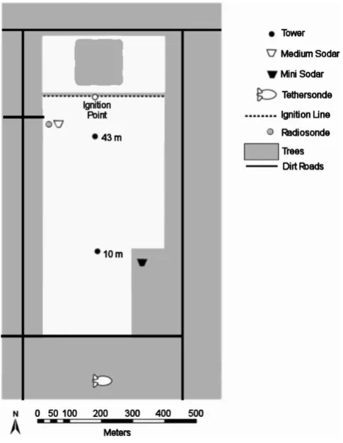
Figure 1 shows the experimental layout with instrument locations. The key platforms included a multi-level 43 m mi-crometeorological flux tower located in the middle of the fuel bed and a similarly instrumented, but shorter, 10 m tower located 300 m downwind from the 43 m main tower. These two towers are hereafter referred to as MT (for main tower) and ST (for short tower). In addition to MT and ST, a teth-ered balloon system was deployed on the downwind edge of the burn block to measure temperature, humidity, and wind speed and direction at five altitudes up to 150 m above ground level (a.g.l.). Two sodars were also used: one was a medium-range system located on the northwest corner of the fuel bed, and the other a mini-sodar located at the southeastern corner of the burn block. Additionally, a radiosonde was released at the edge of the burn block, providing a full in situ verti-cal sounding of temperature, humidity, wind speed and wind direction. Video and time-lapse photography were used to record fire behavior and the spread rate of the fire front. The heights of the sensors used in this study are summarized in Table 1. For the full description of the FireFlux instrumen-tation, the reader is referred to Clements et al. (2007) (their Table 1).
3 Model description
WRF-SFIRE (Mandel et al., 2009, 2011) combines the Weather Research and Forecasting Model (WRF) with a
Fig. 1. Instrument locations and the layout of the FireFlux
experi-ment. White area indicates grass.
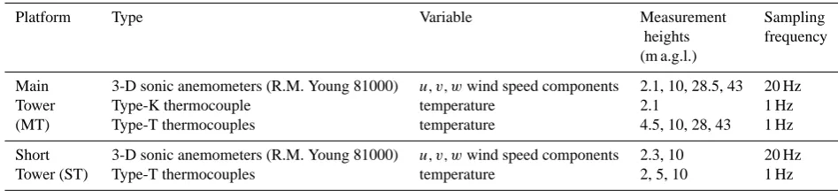
Table 1. Summary of instrumentation used for model validation.
Platform Type Variable Measurement Sampling
heights frequency
(m a.g.l.)
Main Tower (MT)
3-D sonic anemometers (R.M. Young 81000) u, v, wwind speed components 2.1, 10, 28.5, 43 20 Hz
Type-K thermocouple temperature 2.1 1 Hz
Type-T thermocouples temperature 4.5, 10, 28, 43 1 Hz
Short Tower (ST)
3-D sonic anemometers (R.M. Young 81000) u, v, wwind speed components 2.3, 10 20 Hz
Type-T thermocouples temperature 2, 5, 10 1 Hz
properties such fuel mass, depth, density, surface-to-volume ratio, moisture of extinction, and mineral content. The model supports point, instantaneous line, and “walking” ignitions. The SFIRE model is embedded into the WRF modeling framework, enabling easy setup of idealized cases or real cases requiring realistic meteorological forcing and a de-tailed description of the fuel types and topography. The nest-ing capabilities of WRF (not used in this study) allow for running the model in multi-scale configurations, where the outer domain, set at relatively low resolution, resolves the large-scale synoptic flow, while the gradually increasing res-olution of the inner domains allows for realistic representa-tion of smaller and smaller scales, required for realistic ren-dering of the fire convection and behavior. The SFIRE model is available from openwfm.org. A limited version from 2010 is available in WRF release as WRF-Fire, as documented in OpenWFM (2012) and discussed in Coen et al. (2013).
4 Model setup
The WRF modeling framework is used for routine numerical weather prediction in the United States, and its incorpora-tion in WRF-SFIRE allows for detailed descripincorpora-tions of the land use and fuel types (Beezley et al., 2010; Beezley, 2011). In this study, these capabilities were extended to the use of standard land surface models, custom topography, and land use and fuel categories (defined in external files), without the need of the WRF preprocessing system. The aerial picture of the experimental site, model domain boundary, land use, fuel map, and ignition line are presented in Fig. 2.
The fuel map used in the WRF-SFIRE FireFlux simula-tion was initialized with the map of land use derived from an aerial Google Earth picture and simplified to two USGS land use types: mixed forest and grassland. The grass fuel was designated as tall grass fuel, category 3, and the sur-rounding area as noncombustible fuel, category 4 (Anderson, 1982). More details about the fuel characteristics are given in Table 2. Model surface properties defaulted to either one of these two fuel categories. The grass roughness length was de-termined to be 0.02 m according to the pre-fire wind profile measurements from the FireFlux experiment.
Fig. 2. (a) Aerial picture of the FireFlux area with the domain
boundary marked in red; (b) “land use” field from WRF input (red signifies grassland; blue signifies mixed forest) with locations of main tower (MT; green dot), short tower (ST; white dot), and igni-tion line (white dashed line).
The[x, y, z]dimensions of the model domain are [1000 m, 1600 m, 1200 m]. The WRF atmospheric computations were performed on a regular horizontal grid of 10 m spacing and of non-uniform vertical-grid spacing, stretched using a hyperbolic function, varying from 2 m at the surface to al-most 34 m at model top. The fire model mesh was 20 times finer than the atmosphericx, ymesh, which translates into a 0.5 m horizontal grid spacing. The computational details are presented in Table 2.
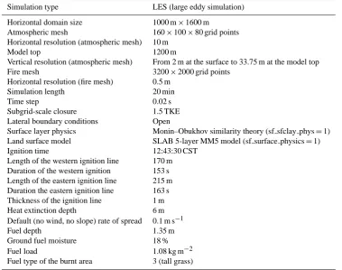
Table 2. Details of the numerical setup used for the FireFlux simulation.
Simulation type LES (large eddy simulation)
Horizontal domain size 1000 m×1600 m
Atmospheric mesh 160×100×80 grid points
Horizontal resolution (atmospheric mesh) 10 m
Model top 1200 m
Vertical resolution (atmospheric mesh) From 2 m at the surface to 33.75 m at the model top
Fire mesh 3200×2000 grid points
Horizontal resolution (fire mesh) 0.5 m
Simulation length 20 min
Time step 0.02 s
Subgrid-scale closure 1.5 TKE
Lateral boundary conditions Open
Surface layer physics Monin–Obukhov similarity theory (sf sfclay phys=1)
Land surface model SLAB 5-layer MM5 model (sf surface physics=1)
Ignition time 12:43:30 CST
Length of the western ignition line 170 m
Duration of the western ignition 153 s
Length of the eastern ignition line 215 m
Duration the eastern ignition line 163 s
Thickness of the ignition line 1 m
Heat extinction depth 6 m
Default (no wind, no slope) rate of spread 0.1 m s−1
Fuel depth 1.35 m
Ground fuel moisture 18 %
Fuel load 1.08 kg m−2
Fuel type of the burnt area 3 (tall grass)
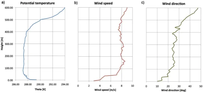
the surface, and neutral above and up to approximately 400 m a.g.l. The wind was northerly at 3 m s−1 for the first 2 m a.g.l., and increasing in magnitude with height to ap-proximately 7 m s−1at 50 m a.g.l. and becoming more north– northwesterly. At higher levels, up to 400 m, wind speed was fairly uniform, averaging about 8 m s−1. There was a marked deviation in wind speed and direction at approxi-mately 50 m a.g.l. The reason for this is unknown, but is pre-sumed to be an artifact of combining tower and tethersonde data. However, this deviation was not removed from the data set.
WRF-SFIRE’s “walking ignition” option was used to em-ulate the start of the fire. Fire line ignition started at the ap-proximate center of the burn area (see Fig. 1) and progressed laterally at the speed estimated by GPS data collected during the actual ignition procedure. Since the GPS unit recorded only one ignition branch, the timing of the other branch was based on data collected during a walk along the ignition line after the actual ignition procedure. The overall length of the ignition line was 385 m. The ignition procedure took about 2.5 min, while the whole burn took about 17 min. More de-tails on the ignition procedure are given in Table 2.
In previous versions of WRF-SFIRE, a point ignition was modeled by setting a fixed circle on fire at once, with the circle size at least the size of a horizontal fire cell, while a walking ignition was modeled as a succession of circles.
In this study, such a walking-ignition scheme produced an ignition line at least 0.5 m wide, while FireFlux’s dip torch ignition line was likely thinner; the 0.5 m wide ignition strip caused the initial fire propagation to be too fast. Therefore, to prevent this, the WRF-SFIRE ignition model was revised to apply a slower initial subgrid ROS during the time period from ignition until the fire is large enough to be visible on the fire mesh, after which time the propagation mechanism based on the Rothermel formulation takes over. See Sect. 3.6 in Mandel et al. (2011) for the details of the ignition imple-mentation in the framework of the level-set method.
In addition, to achieve a realistic fire propagation rate be-tween ignition of the initial fire line and FFP at the MT, the Rothermel default no-wind fire line rate of spread (ROS) was increased from 0.02 m s−1to 0.1 m s−1(Table 2). This ROS is applied when there is no wind component perpendicular to the leading edge of the subgrid-scale combustion zone. Com-parison with flank ROS simulated by FIRETEC (Cunning-ham and Linn, 2007) for grass fires suggests that 0.02 m s−1 is an order of magnitude too small. The five-fold increase in no-wind ROS also resulted in more realistic spread along the fire’s flanks and back (upwind) side.
Fig. 3. Initial atmospheric profiles used for model initialization: (a) potential temperature, (b) wind speed, and (c) wind direction.
but precise measurements were not taken. For the sake of this study, we set it to 1.35 m.
Another fire model feature that was set to provide good agreement with observations was the e-folding extinction depth used to parameterize the transport of sensible, latent, and radiant heat from the fire’s combustion zone into the near-surface layers of WRF. In WRF-SFIRE, the total heat liberated into the atmosphere by the fire is released vertically into the model atmosphere using the e-folding extinction depth. Sun et al. (2006, 2009), following Clark et al. (1996b), also used this simple extinction depth approach to treat the fire–atmosphere heat exchange. Sun et al. (2006) found that plume-averaged properties were sensitive to the choice of ex-tinction depth; too large an exex-tinction depth underestimated important near-surface properties just above the combustion zone, such as temperature excess and vertical plume veloc-ity; too small an extinction depth produced agreement be-tween observed and model-predicted plume-averaged tem-peratures, but less agreement between observed and model-predicted plume-averaged vertical velocities just above the surface. There exists therefore no unique value for this pa-rameter. In this study the flame length estimate of 5.1 m by Clements et al. (2007) was used to set the extinction depth to 6 m.
Unfortunately, the infrared video camera used to record the fire experienced technical problems, and continuous in-frared imagery of the location and spread rate of the fire head is not available for analysis. Wind and air tempera-ture measurements are used instead to represent head fire spread, plume properties, and behavior. Note that the Fire-Flux temperatures used in this study were measured by a type-T thermocouple sampled at 1 Hz (Clements et al., 2007; their Table 1). FireFlux temperatures were also measured at 2.1 m a.g.l. at the MT and 2.3 m a.g.l. at the ST with a type-K fine-wire 20 Hz thermocouple. Because the fine-wire thermo-couples failed at times, and measurements below 2.5 m a.g.l. were possibly affected by precautions taken to shield these thermocouples (i.e., grass was mowed around the towers)
from damage by the fire, these data are not used in the evalu-ation of WRF-SFIRE output.
Horizontal atmospheric grid resolution limits the fre-quency of the fluctuations in temperatures or flow that the model can resolve. For the atmospheric horizontal grid size of 10 m, the shortest disturbance or fluctuation that the model resolves is assumed to have an approximate length of 40 m. If this perturbation travels at 8 m s−1, roughly the peak wind speed observed during FireFlux, the effective frequency of disturbance resolved by the model is 1/(8/40) or 0.2 Hz. Therefore, the WRF-SFIRE output frequency was 0.2 Hz (i.e., results were saved every 5 s), and a 5 s moving average was applied to the FireFlux measurements for direct compar-ison to model results.
5 Results
5.1 Fire spread
Fire-spread rates are determined by the time series of 4.5 m a.g.l. at the MT and 5 m a.g.l. at the ST simulated and observed air temperatures shown in Fig. 4 (gray lines show 1 Hz thermocouple data, and black lines show 5 s averaged 1 Hz thermocouple data). Model results are interpolated ver-tically between second (4.49 m) and third (7.7 m) model lev-els. The timing of FireFlux’s FFP through the MT is indi-cated by rapidly rising and falling air temperatures in the time series. This timing is well captured by WRF-SFIRE. The simulated MT air temperature reached the peak value at 225 s after the ignition, while observations indicate a peak temperature just 6 s earlier. Timing of the FFP through the ST is also well captured by the model. There is only a 5 s de-lay with respect to the observations, and the simulated ROS between the two towers is 1.61 m s−1, exactly the observed
Fig. 4. Time series of the 4.5 m a.g.l. air temperature at the location
of the main tower (MT) and 5 m a.g.l. air temperature at the short tower (ST). Gray lines show 1 Hz measurements, black lines 5 s av-eraged values, and symbols (diamond and square) model data.
5.2 Thermal plume structure
In terms of magnitude, the agreement between observed and simulated temperatures is relatively good. Figure 4 indicates that the WRF-SFIRE’s peak air temperature at the MT is 35 K warmer than the 5 s averaged measurements and 88 K cooler than the maximum temperature from the 1 Hz ther-mocouple data. The data from the type-T therther-mocouple (sampling frequency 1 Hz) at 4.5 m a.g.l. were used. How-ever, we believe, based on a comparison between tempera-tures taken from the type-T and type-K fine-wire thermocou-ples at the sonic locations (2.1 m on MT and 2.3 m on ST), that the type-T thermocouple, after 5 s averaging, tended to underestimate temperatures by sometimes as much as 90 K and 32 K. This suggests that simulated air temperatures are within only 3 K of temperatures measured with the faster responding fine-wire thermocouple. Figure 4 shows that ST thermocouple temperatures are slightly higher than those at MT. Temperature maxima are 304◦C at the ST and 295◦C at the MT. The simulated peak temperature at the ST is also 9 K higher than the simulated peak temperature at the MT. These differences are eliminated by 5 s averaging. The filtered peak air temperature is 172◦C at the MT and 171◦C at the ST. The model again underestimated the 4.5 m a.g.l. air temperature at the ST by 88 K, almost exactly the bias between model and 1 Hz temperature data at MT. Compared with the fil-tered data, the model overestimated the ST air temperature by 45 K.
Figure 5 is the same as Fig. 4 except for time series plots at the MT at 2 m, 10 m, 28 m and 43 m a.g.l., and demonstrates how well WRF-SFIRE plume’s vertical tem-perature profile matches the tower thermocouple temper-ature measurements. Tower tempertemper-atures before and after fire passage remain steady and deviate very little from the background temperature. This behavior is well predicted by WRF-SFIRE. Figure 5a and b show that temperatures in the WRF-SFIRE plume begin to rise above and then fall to am-bient (no fire) values at virtually the same times as FireFlux plume values: fire-plume arrival and passage are practically identical for both measured and simulated plumes. However, changes in observed temperature with fire passage do differ
0 50 100 150 200 250 300
T10m
MT
[
C
]
T 10m MT TC T 10m MT srx 20 5s av. T10m MT TC a) Temperature 2.1m main tower (fuel)
b) Temperature 10m main tower
c) Temperature 28m main tower
d) Temperature 43m main tower
Fig. 5. Time series of the thermocouple air temperatures at the
lo-cation of the MT at (a) 2.1 m, (b) 10 m, (c) 28 m, and (d) 43 m a.g.l. Gray lines show 1 Hz measurements, black lines 5 s averaged val-ues, symbols (open circles, triangles, squares, and diamonds) model data.
which model variables are averaged. These model oversim-plifications may also be responsible for the unrealistic lack of spatial and temporal temperature (and wind) fluctuations in the WRF-SFIRE plume, especially at levels>10 m a.g.l. Differences between model and FireFlux thermocouple tem-peratures are to a great degree eliminated by 5 s averaging. When the WRF-SFIRE temperature time series in Figs. 4, 5a and b are compared to the 5 s moving mean of the FireFlux temperatures, a greater level of agreement is seen. To a mod-erate degree, WRF-SFIRE overpredicts fire plume tempera-tures (by 35 K) at 4.5 m a.g.l. but agrees within 25 K at all other levels.
Figure 5c and d show the upper levels of the warm, downwind-tilted FireFlux plume arriving, respectively, at the main tower just at and after 100 s into the experiment. Plume arrival occurs slightly sooner at 28 m a.g.l. compared to 43 m a.g.l., and plume passage occurs later at 28 m a.g.l. compared to 43 m a.g.l. Although the WRF-SFIRE tempera-ture time series in Fig. 5c and d do not show plume arrival at lower levels first, the temporal differences in fire-plume ar-rival and passage between FireFlux and WRF-SFIRE at these al these levels (AGLs) are slight. Measured plume tempera-tures as well as the 5 s moving means during fire passage show significant fluctuations in magnitude at both 28 m and 43 m a.g.l. Fluctuations of this magnitude are not unexpected in the upper portion of an entraining, turbulent fire plume. The results indicate that even though the WRF-SFIRE did not capture these high-frequency fluctuations, it predicted the FireFlux peak temperatures at 28 m and 43 m a.g.l. very ac-curately (with 9 K and 1 K bias, respectively). Time of plume arrival is well predicted by WRF-SFIRE at the 43 m level and underpredicted by approximately 20 s at the 28 m level. The abrupt falloff in measured plume temperatures as the up-wind edge of the plume passes the tower is well represented in the WRF-SFIRE time series. Temperature measurements at 43 m show that air temperatures remain slightly elevated above ambient values even after the plume has passed, while temperatures measured just 1 m below (not shown) and sim-ulated by WRF-SFIRE drop immediately to pre-fire ambi-ent values. However, local variation of plume properties in the upper levels of a highly turbulent convective plume is not unrealistic, which suggests that this level of agreement between predicted results and measurements is remarkable. Clements (2010) reports that the greatest temperature differ-ence and variability compared to ambient air temperatures occurred at 10 m a.g.l., where entrainment of ambient air is possibly the greatest.
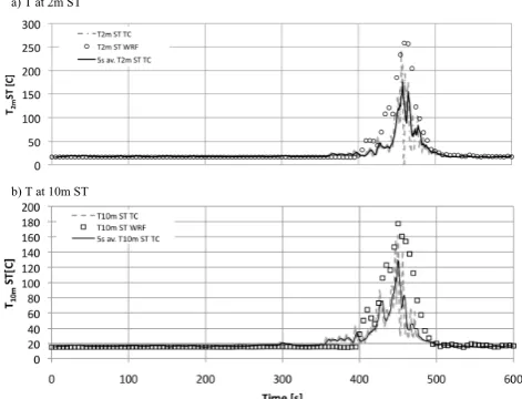
Figure 6 is the same as Fig. 5 except for time series plots at the ST at 2 m and 10 m a.g.l. Fire-plume arrival and passage are practically identical for both measured and simulated plumes. However, WRF-SFIRE overestimates plume tem-peratures at these two levels. Simulated fire-plume temper-atures are within 25 K of the 1 Hz observations, but greater by 82 K at 2 m a.g.l. and 45 K at 10 m a.g.l. than peak 5 s moving means, and they remain elevated for a significantly
a) T at 2m ST
b) T at 10m ST
Fig. 6. Time series of the thermocouple air temperatures at the
lo-cation of the short tower (ST) at (a) 2 m and (b) 10 m. Gray dashed lines show 1 Hz measurements, black solid lines 5 s averaged val-ues, and symbols (open circles and squares) model data.
longer time than measured ones. Due to the lack of infrared video camera recordings, it is difficult to report the actual fire front depth. However, differences in the time periods be-tween simulated and observed fire plume temperature values suggest that the model is overestimating the thickness of the fire front. Using a 100 kW m−2heat release rate threshold, the simulated fire front thickness at the ST is estimated as 45 m, which appears to be too large. Note that, at the MT, the fire front thickness is estimated to be half as large, only 27.5 m thick. This 45 m front thickness is likely responsible for an unreasonably higher fire heat release and consequently unrealistically higher model fire-plume temperatures at the ST.
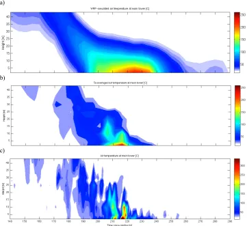
14 in the width of the fire zone as evident in Figure 7 a). a)
b)
c)
Figure 7. Air temperatures at the MT as a function of time: a) WRF-simulated, b) thermocouple 5s averaged, c) thermocouple raw (1s).
Nonetheless, Figure 7 shows that WRF-Sfire successfully captured the plume’s downstream tilt, the arrival between 180 to 200s of fire-warmed surface air, and the passage of the fire-warmed surface air at approximately 260s, with the low-level near-surface warmest volume of air arriving approximately 10s later at the MT than observed. Contoured WRF results also show that the 15m vertical extent of the warmest (greater than 100C) plume temperatures matches the observations presented in Figure 7 b).
Fig. 7. Air temperatures at the MT as a function of time: (a) WRF-simulated, (b) thermocouple 5 s averaged, and (c) thermocouple raw (1 s).
width of the temperature perturbation that can be resolved. The averaging of heat released by the fire over the whole at-mospheric grid-volume affects the appearance of the fire sig-nal on the atmospheric mesh. Regardless of how narrow the fire front on the fine fire mesh is, as the fire crosses two ad-jacent atmospheric cells, the heat released is averaged over the two cells. As a consequence the minimum width of the fire-related thermal signal seen on the atmospheric grid is two atmospheric grid spaces, which in this study is 20 m, far greater than the estimated 6.2 m fire-front thickness. The fuel burn rate used in WRF-SFIRE is the same for all fuel types, which may result in a too-long fuel residence time for quickly burning fuels like grass. This may also result in the overesti-mation in the width of the fire zone as evident in Fig. 7a.
Nonetheless, Fig. 7 shows that WRF-SFIRE successfully captured the plume’s downstream tilt, the arrival between 180 and 200 s of fire-warmed surface air, and the passage of the fire-warmed surface air at approximately 260 s, with the low-level near-surface warmest volume of air arriving ap-proximately 10 s later at the MT than observed. Contoured WRF results also show that the 15 m vertical extent of the warmest (greater than 100◦C) plume temperatures matches the observations presented in Fig. 7b.
5.3 Dynamical plume structure
5.3.1 Fire-induced horizontal winds
WRF-SFIRE computes the ROS based on coupled fire– atmosphere winds at the fire line. It is crucial, therefore, for realistic prediction of wildfire behavior that WRF-SFIRE captures accurately the fire–atmosphere interaction and evo-lution of the surface flow at the fire line. To evaluate for this, model results are compared to FireFlux wind measure-ments. Heat and temperature extremes did cause some minor damage and instrument failure during FireFlux. The sonic anemometer at the ST broke during the FFP. Therefore in the analysis of the WRF-SFIRE plume dynamics, data from the MT, which captured more of the vertical plume structure, are used.
a) Wind speed 2m main tower
b) Wind speed 10m main tower
c) Wind speed 28m main tower
d) Wind speed 43m main tower
0 2 4 6 8 10 12 14
0 100 200 300 400 500 600
WS
43m
[m
/s]
Time2[s]2
WS243m2MT WS243m2MT2WRF 5s2av.2WS243m2MT
Fig. 8. Time series of horizontal wind speed (WS) at MT levels: (a) 2 m, (b) 10 m, (c) 28 m, and (d) 43 m. Gray dashed lines show
1 Hz measurements, black solid lines 5 s-averaged values, symbols (circle, triangle, diamond, square) model data at the four MT mea-surement levels.
a distinct rise and fall in wind speed as it was with temper-ature, and this is especially true at upper-tower levels 28 m (Fig. 8c) and 43 m (Fig. 8d). At 2 m a.g.l. (Fig. 8a) just before fire passage, the wind speeds rise, reaching 6 to 12 m s−1 dur-ing fire passage, and then fall to values slightly greater than ambient just after fire passage. Wind speeds at 10 m a.g.l. (Fig. 8b) show similar behavior except that peak values are lower, approximately 4 to 8 m s−1. Both measured and
5-point moving means in Fig. 8c and d show strong fluctuations in wind speed as the FireFlux plume passes the MT. At these levels the FireFlux measurements vary in magnitude and do not display a single peak value.
There is agreement in Fig. 8 between the WRF-SFIRE results and the FireFlux 5-point moving means. Figure 8a and b show how, during fire passage, although wind speeds
fluctuate throughout, the overall trend is well captured by WRF-SFIRE. Simulated and observed wind speeds rise, peak, and then fall. At 10 m a.g.l. the maximum simulated wind speed matches almost exactly the filtered observations (with a 0.2 m s−1negative bias), while at 2 m a.g.l. the model overestimates the peak wind speed by only 1.2 m s−1. Nei-ther time series of observed or model wind speeds at the higher elevations display a strong response to the fire plume’s passage. At these levels fluctuations in ambient wind speed are similar in amplitude to those associated with fire plume passage, making the quantification of the fire’s effect on the wind speed practically impossible. It can be said that before plume passage WRF-SFIRE wind speeds at 28 m and 43 m are in overall mean agreement with FireFlux observations. After plume passage, WRF-SFIRE wind speeds at 28 m and 43 m are overall greater than FireFlux observations. As dis-cussed before, considerable variation of plume properties in the upper levels of a highly turbulent convective plume is not unrealistic, which makes even this level of agreement be-tween predicted results and measurements acceptable.
The WRF-SFIRE wind speeds shown in Fig. 8 behave as described by Clements et al. (2007). As the fire front ap-proaches the MT, the surface wind speed more than triples, and before the horizontal wind increase there is a brief pe-riod of calm that, as suggested by Clements et al. (2007), is associated with horizontal convergence in the flow ahead of the fire line that coincided with increased vertical motion. Clements et al. (2007) have the wind direction shifting from northeasterly to southerly at 12:45:50 CST, approximately 50 s before the head fire reached the MT. As the fire front passed the MT at 12:46:40 CST, wind direction switched back to ambient northerly flow, while wind speeds increased from approximately 3 m s−1to over 10 m s−1. At the upper
levels of the MT, there were large increases in wind speed, but not as long in duration as observed at the surface. While the vertical profile of the ambient wind shows wind speed increasing almost logarithmically with height, both observa-tions and the simulation indicate that, during passage of the fire front, the maximum wind speed occurs at the surface and decreases in magnitude with height.
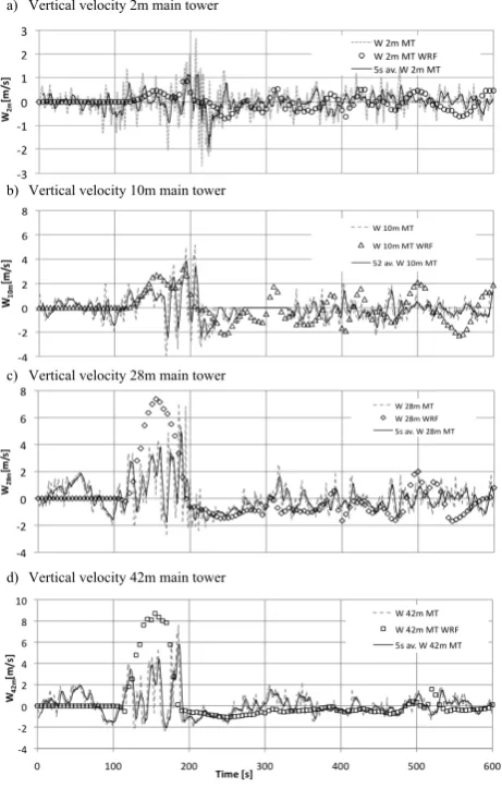
5.3.2 Fire-induced updraft
a) Vertical velocity 2m main tower
b) Vertical velocity 10m main tower
c) Vertical velocity 28m main tower
d) Vertical velocity 42m main tower
Fig. 9. As in Fig. 8 except for vertical wind speed.
and downdraft of similar strength are still captured realisti-cally by the model.
The model and FireFlux observations displayed in Fig. 9 show that the maximum updraft velocity associated with plume passage increases with height, while the downdraft stays at a similar strength at all heights. Figure 9c and d indi-cate that the model overestimated upward velocity at higher levels. The underestimation in the simulated horizontal wind speed at these levels shown by Fig. 8c and d could indicate that the modeled plume was not tilted downstream enough (was too vertical), so that the vertical wind component was overestimated while the horizontal one was underestimated. However, a more vertical plume would result in delayed plume arrival at higher elevations. Figure 9c and d indicate that this is not the case; the timing of the model updraft ve-locity peaks is captured correctly at 28 m and 43 m a.g.l. It is more likely that the discrepancy between measured and simulated vertical velocities at upper levels results from the model overestimating the fire front depth, consequently af-fecting the amount of total heat released into the atmosphere, and therefore the plume updraft speeds. At low elevations, for reasons just discussed, simulated updraft velocities are
numerically limited, so they match well with observations. At higher elevations, the model responds more freely to the excessive heating by increasing the vertical velocity within the plume.
5.3.3 Spatial structure of the fire-induced flow
Based on the good agreement between FireFlux observations and WRF-SFIRE results seen in Figs. 4 to 9, a more detailed analysis of the possible dynamics responsible for FireFlux behavior as the fire passed the MT and ST may be attempted using the WRF-SFIRE simulation. Here model flow proper-tiesw, the verticalzvelocity component, and|Vh|, the
mag-nitude of the horizontal wind velocity, are examined, along with the following wind features:
δ=∂u
∂x+ ∂v ∂y,
the divergence in the horizontalx–yflow, and
ζx=∂w
∂y − ∂v ∂z,
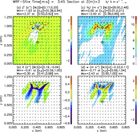
thexcomponent of vorticity due to the development of shear in they–zflow. Hereu, v,andw are thex, y,andz com-ponents of the flow. The separation or coming together of flow parcels in thex–yplane is described byδ,whereδ >0 signifies divergence andδ <0 signifies convergence of flow parcels. The spin or rotation of flow parcels in they–zplane is described byζx, whereζx>0 signifies cyclonic or coun-terclockwise rotation and ζx<0 signifies anticyclonic or clockwise rotation of flow parcels. Figures 10 and 14 are
x–y cross sections that illustrate WRF-SFIRE behavior at 3 m a.g.l. (the second height level in the model simulation) at two times: 3:45 [min:s] when the fire front reached the MT; and 7:45 [min:s] when the fire line reached the ST. Figures 11 and 15 arey–zcross sections that illustrate the WRF-SFIRE behavior atx=465 m (location of the towers) at these two times.
Figure 10 shows all of the flow features described by Clements et al. (2007) for 3:40 [min:s]. As the fire front ap-proached the MT, the surface wind speed more than tripled, and before the horizontal wind increase, there was a brief pe-riod of calm associated with horizontal convergence ahead of the fire line that coincided with increased vertical motion. Wind vectors in Fig. 10 show clearly how, just ahead of the MT and the fire head, the direction and speed of the horizon-tal wind changed from ambient wind conditions of mainly northerly flow of approximately 3 m s−1 to the almost
Fig. 10. Horizontal cross sections for 3 m a.g.l. of (a) horizontalx vorticityζx(s−1), (b) horizontal divergenceδ(s−1), (c) speed of horizontal wind|VH|(m s−1), and (d) vertical velocityw(m s−1)at
3:45 [min:s] into the WRF-SFIRE simulation. Magnitudes of each contour are indicated by colors in bar plots on the right. For each field, minimum and maximum values, plus their (x, y)positions on cross section are given. Vectors denote wind components inx–y plane where magnitude is scaled as indicated in the top right corner of plot. Black dotted contour lines delineate the surface fire perime-ter. Note that the (aspect) ratio between the height of each plot to its width is not equal to one. Plots show features lengthened in the ydirection compared to thexdirection. The (x, y)locations of the MT and ST are indicated by black diamonds.
behind and along entire leading edge of the fire front. Hori-zontal convergence and vertical velocity are most significant immediately out ahead of the fire front. Convergence in the horizontal wind is strongest at the base of the narrow up-draft. At the time of FFP, in agreement with observations, the WRF-SFIRE horizontal wind speeds increased due to the fire-induced updraft and surface convergence, while back-ground winds outside the burn perimeter remained constant. Figure 10 displays additional structure to the flow. Fig-ure 10a indicates positive x-vorticity (ζx) at the MT lo-cation and the leading edge of the fire front, and negative behind. Downstream flow features are associated with hor-izontally oriented convective rolls. Out ahead of the fire head are divergence, weak horizontal wind, and downward motion, between strong convergence, significant horizontal wind speeds, and upward motion. The convergence out ahead of the fire front on either side of the fire head may be respon-sible, in part, for the observation of Clements et al. (2007) that the convergence zone was farther ahead of the fire front than previously thought. The model shows the fire head mov-ing towards the south–southwest as it reaches the MT.
Fig. 11. As in Fig. 10 except for vertical y–z cross sections at x=465 m. The bottom plot displays the energy release rate (ERR) (kW m−2)from the surface fire as a function ofy. Maximum rear and head (R/H) distances (km) advanced by the fire are given, along with fire flux (ERR) values at the surface locations of the MT and ST. The top locations of the MT and ST are indicated by black dia-monds.
Figure 11 showsy–zcross sections through the MT and fire head at time 3:40 [min:s]. By comparing Fig. 10a and d to Fig. 11a and d, it is seen that the significant counterclockwise (clockwise)ζxahead of (behind) the leading edge of the fire head coincides with ∂w∂y <0∂w∂y >0as part of the model plume’s updraft (relatively weaker trailing downdraft).
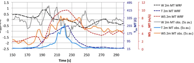
Fig. 12. Time series from the MT of the simulated (dashed lines) and observed (solid lines) updraft velocity (W), temperature (T) and horizontal wind speed (WS) at 2 m. Observational results are presented as 5 s averages of the original 1 Hz data.
Fig. 13. Verticaly–zcross section atx=465 m, 225 s into simula-tion. Vectors denote wind components iny–zplane where magni-tude is scaled as indicated in the top right corner of plot. Contour lines represent air temperature (◦C), and the magnitude of each con-tour line is indicated by the color bar on the right side of the plot. The red thick line shows the ERR (W m−2)computed on the fire grid.
Clements et al. (2007) and Fig. 11a suggest a horizon-tal vortex immediately in front of the fire front at the MT. Clements et al. (2007) also describe soot particles (seen in video and time-lapse photography) dropping out in front of the head fire during the fire passage at the MT. Figure 11a indicates two regions of counterclockwise rotation: a weaker one at upper levels near 0.12 km a.g.l., and a stronger one at the surface just downstream of the fire front aty=0.96 km. It may be that the soot particles observed by Clements et al. (2007) were entrained into the plume by the stronger sur-face horizontal vortex, carried up into the plume by this cir-culation, and then dropped out downstream of the fire.
Close-ups of model results and observations of tempera-ture andw values during FFP at the MT are displayed in Figs. 12 and 13. Peaks in the observed and simulated verti-cal velocity (Fig. 12; gray solid and dashed black lines, re-spectively) arrive earlier at the MT than peaks in observed and simulated temperature (Fig. 12; solid and dashed blue lines, respectively). Figure 13 shows that the WRF-SFIRE updraft core is situated ahead of the fire front, whose posi-tion is identified by the maximum in the ERR. The strongest
surface convergence is associated with calm surface wind speed and located at the base of the plume’s updraft, and both model results and observations suggest that these fea-tures are located ahead of, not in or above, the fire’s head. Because of the downstream shift, ahead of the fire front, by convergence in the horizontal flow and associated upward motion, fire spread is driven by a local fire-induced wind (Fig. 12; dashed red and solid orange lines) of much greater magnitude than the ambient one. Figure 12 shows that peaks in the simulated wind speed (dashed red line) and tempera-ture (dashed blue line) are collocated. Strong surface winds cross the fire line, advecting fire-heated air downwind, where the warmed, buoyant air converges to form the base of the fire’s plume. Note that the maximum ERR of∼2 MW m−2 at the MT seen in Fig. 13 is the WRF-SFIRE instantaneous fire-grid mesh-averaged value. Using 2 m a.g.l. thermocouple and vertical wind measurements, Clements et al. (2007) esti-mated 1 MW m−2as a heat flux maximum. Note that the pre-vious atmospheric grid-averaged ERR of∼1.216 MW m−2 compared to the 2 m fire-mesh ERR of 2 MW m−2indicates the sensitivity of the magnitude of model properties to grid-volume averaging.
Fig. 14. As in Fig. 10 except for 7:45 [min:s] into the WRF-SFIRE
simulation.
(3 m s−1) wind conditions (their Fig. 3). Figure 14 shows
complex patterns toζx,δ, andw, not just out ahead of the fire, but over the entire area enclosed by the fire perimeter. There are alternating strips or streaks of up/down vertical motion coincident with convergence/divergence in the hor-izontal flow field. These appear to be organized horhor-izontal rolls or eddies embedded in the burning area and aligned with the mainly northerly background flow, similar to the convec-tive instabilities known as “cloud streets” that are common in the atmosphere (Brown, 1980; Etling and Brown, 1993). It should be noted that these fire “streets” did not develop until the Rothermel default no-wind fire ROS was increased from 0.02 m s−1to 0.1 m s−1. There are no FireFlux data to vali-date this result, but this flow pattern is similar to the convec-tive and radiaconvec-tive heating patterns seen in the Cunningham and Linn (2007) FIRETEC simulations of 100 m long grass fire lines (their Fig. 4). These model results suggest that the heat released by actively moving fire flanks and back is es-sential to the production of these dynamic “fingers.”
Figure 15 showsy–z cross sections through the ST and fire head at time 7:45 [min:s]. As before, significant coun-terclockwise (clockwise) ζx ahead of (behind) the leading edge of the fire head coincides with ∂w∂y <0 ∂w∂y >0as part of the model plume’s updraft (relatively weaker trail-ing downdraft). The wind vectors do not show winds shift-ing to undisturbed steady northerly flow once the fire front has passed. Between the front and backfire lines, at 0.58 and 1.12 km in they direction, respectively, flow is disturbed in the region of the fire showing what is likely the result of the convective instabilities or “fingering” seen in Fig. 14. The
Fig. 15. As in Fig. 11 except for 7:45 [min:s] into the WRF-SFIRE
simulation.
model results indicate that, just as the fire front passed the ST, a period of downward motion occurred. The position and distribution of heating rates in the fire’s head and rear line are seen in the bottom plot in the figure. Averaged on the WRF atmospheric grid mesh, the maximum ERR (energy release rate) was 1045 kW m−2at the fire’s front (bottom plot in Fig. 15).
As before at 3:45 [min:s], wind speeds are largest at upper levels in the plume. Figure 15 shows the strongest vertical motion and horizontal wind at approximately 0.45 km and 0.46 km a.g.l. Although there are no FireFlux data to validate these ST model results, they are consistent with the plume and fire behavior seen in Fig. 11 for the MT. Model results (not shown) indicate that maximum vertical wind speeds are always found below 400 m a.g.l., while the largest vertical extent of the plume is approximately 800 m a.g.l.
6 Discussion
It is understood that, after initial ignition, wildfires ex-perience an “acceleration” or growth phase, before reach-ing an “equilibrium” or quasi-steady rate of spread (Cheney and Gould, 1997). WRF-SFIRE was coded therefore to take this fire growth phase into account, using arrival time at the MT as a guide. By taking the fire’s initial growth phase into account, the simulated fire propagation times to the MT com-pared very well to the observations.
Current operational fire-spread models are formulated for head-fire propagation where, typically, a single generalized default no-wind spread rate is applied along both the fire’s back and flanks. But as Mell et al. (2007) demonstrate, there is no general flank- or back-fire-spread rate; modeling the evolution of the entire fire line is a greater challenge, due to the different spread mechanisms, than modeling the be-havior of just the head fire. Rothermel’s default no-wind rate spread value for the grass of properties shown in Table 2 is 0.02 m s−1, which ensures essentially zero spread along the
back or flanks of a fire. Used in preliminary WRF-SFIRE runs, this no-wind value did not provide good agreement with the FireFlux fire line’s arrival at the ST. The fire front was so skewed that the ST was passed by a fire flank rather than its head. Therefore, in order to achieve realism of the FFP, this value was increased to 0.1 m s−1. However, this impor-tant parameter impacts the heat release rate, and the result in this study was active flank- and back-fire spread with dis-cernible consequences for fire plume properties and behav-ior. If flanking fire and backing fire spread are due to differ-ent mechanisms, then it is in general not appropriate to apply a single no-wind fire-spread value as done in the Rothermel fire-spread formulation. It was not possible however to de-termine, using available FireFlux observations, if the simu-lated flank and back-fire-spread rates reproduced accurately the entire fire perimeter spread or not. It may be worthwhile to investigate the use of fire-spread formulations other than Rothermel’s in WRF-SFIRE, such as Balbi et al. (2007), that require a relatively small number of input parameters and provide a variable no-wind fire-spread rate depending on these parameters. Also, as suggested by one of the review-ers, the local no-wind ROS could be derived from a separate model like Prometheus by Canadian Forest Service (Tymstra et al., 2010).
A second fire model parameter that impacts heat release is the fuel depth. Clements et al. (2008) estimated 1.5 m as the depth of the grass fuel, whereas in this study, in order to produce agreement between simulated and observed fire behavior, a fuel depth of 1.35 m was used. The Rothermel fire-spread model is particularly sensitive to fuel properties such as moisture content (Jolly, 2007) and the fuel depth. Again, this result suggests that fire growth models other than Rothermel’s should be tested in WRF-SFIRE.
A third important fire model feature is the e-folding extinc-tion depth used to parameterize the absorpextinc-tion of sensible, latent, and radiant heat from the fire’s combustion into the surface layers of WRF. In this study the flame length estimate
of 5.1 m by Clements et al. (2007) was used to set the extinc-tion depth to 6 m, with the result being that the WRF-SFIRE vertical profile of temperature taken at the main tower was in good agreement with FireFlux observations, whereas the vertical profile of vertical velocity shows WRF-SFIRE values larger than those observed. This relatively good temperature agreement suggests that efforts to distinguish explicitly be-tween or to model the different modes of fire–atmosphere heat transfer (conductive, convective, radiative) may not, at substantially greater computational cost, provide substan-tially better plume temperature prediction for a relatively simple grass fire. It is noted, however, that for much more complex crown fires this approach may not be valid.
This study provides the opportunity to suggest the design of future field campaigns used to evaluate or validate numer-ical wildfire models such as WRF-SFIRE. In addition to the observing procedures to measure winds, temperature, humid-ity, and surface pressure, described in Clements et al. (2007, 2008) and Clements (2010), the following are suggestions for field campaign protocol based on the results of this study.
The experimental layout needs to be measured carefully for spatial dimensions, any special geographic features, and tower and equipment positioning. This suggestion is based on the finding that the evaluation of the simulated fire was sensitive to the accuracy of these features and their locations in the WRF-SFIRE model domain. Positioning done with GPS ranges in accuracy from 10–30 cm to (more typical) 1– 5 m, depending on the GPS receiver.
The position of the initial fire line should be clearly marked and reported, and the timing of the walking-ignition well determined. In addition, to ensure uncomplicated initial fire line behavior, the initial fire line should be as perpendic-ular as possible to, ideally, a directionally steady background wind. These suggestions are based on the observation that the evolution of the simulated fire appears to be sensitive to any asymmetry in the timing and positioning of the walking-ignition and prevailing winds.
Note that in this study observations at greater than 1 Hz sam-pling rate were not needed or used to evaluate WRF-SFIRE. A LES is inherently unsteady. There are studies, for exam-ple Chow and Street (2009), that suggest that, for a LES sim-ulation to predict successfully both mean flow and turbulence in the ABL, it should be provided with inflow conditions based on a separate, predetermined turbulent flow database. The ensemble averages of the no-fire WRF-LES and field data turbulent flow results would be used for this purpose.
The placement of the observing platforms relative to the initial fire line and wind field is important. The tower ar-rangement in FireFlux was intended to capture the flow and temperature fields at the fire–atmosphere interface as the fire front traveled with the wind and passed each tower con-secutively (Clements et al., 2008). It is recommended that taller (main) instrumented towers be placed farther down-wind from smaller (shorter) towers. This layout is different from the one used in FireFlux and is based on the observa-tion that the fire line’s behavior and plume are, respectively, relatively simple and small in the early stages, growing more complex and taller with time. Clements et al. (2007) note that an array of towers aligned east–west would have provided a better description of the surface flow and verification by di-rect observation of the fire-induced flow features associated with the combustion-zone winds.
Although a tethersonde system in tower mode with five sondes was deployed during FireFlux, data during the fire are missing due to the loss of the tethered balloon as a result of strong vertical downdrafts during the initial plume impinge-ment on the balloon. These data provide the above-tower (i.e., upper-level) vertical structure of temperature, humidity, and wind in the fire plume, and are especially valuable for a model validation study. Based on WRF-SFIRE results, the maximum plume height was estimated at 800 m a.g.l., which is a height that only a tethersonde system can measure. It is known now from the FireFlux experience just how strong the tether for the tethersonde system needs to be.
A radiosonde launched on-site just before the burn, instead of a few hours earlier, would be most useful for documenting the background atmospheric conditions. Even without any large-scale synoptic forcing, both wind and temperature can change in just a few hours as part of the normal diurnal cy-cle or topography-influenced meteorology. Basic, portable, weather stations located upwind and outside the burn perime-ter would also provide background meteorological measure-ments before, up to, and during the burn.
Multiple digital infrared video and visible SLR cameras can be employed to document smoke and flames. Using a still exploratory method, Clark et al. (1999) show how it is possi-ble to calculate convective-scale velocities and heat fluxes from infrared imagery. Doppler lidar (Banta et al., 1992; Charland and Clements, 2013) can also be used to observe the finer scale kinematics of fire plumes.
The spread of the entire fire perimeter should be mea-sured accurately. In FireFlux, even though orange markers
were placed in the fuel at 10 m intervals from 50 m north to 300 m south of the main tower to aid in head-fire-spread rate determination, this information was not adequate to eval-uate the size and shape of the entire fire perimeter as the fire evolved. Aerial video (recorded from a helicopter) and time-lapse photography can provide information on perime-ter spread, but ideally this information should be supple-mented with measurements from a surface-based thermocou-ple array. In FireFlux, soil temperature thermocouthermocou-ples were buried 3 and 10 cm below the surface, but these were placed only near the base of the MT (Clements et al., 2008). Ther-mocouples capable of measuring temperatures up to 1200◦C, and housed in a (plastic) unit, buried just below (5 cm or so for grass fires, 10 cm for higher intensity burns) the surface, can be used to determine fire line arrival times.
The FireFlux burn lasted for approximately 17 min. As de-scribed in Cheney and Gould (1997), and references therein, the typical fire growth curve for a fire burning under fairly stable fuel moisture and wind conditions takes approximately 30 min before reaching a quasi-steady rate of spread. Ideally, measurements from burns lasting at least that long would be very valuable for evaluating numerical fire behavior predic-tion models such as WRF-SFIRE.
7 Concluding remarks
In this study, FireFlux observations (Clements et al., 2007, 2008; Clements, 2010) – the first comprehensive set of in situ measurements of turbulence and dynamics in an experimen-tal wildland grassfire – were used to evaluate and improve the forecast capabilities of WRF-SFIRE. The various changes made to WRF-SFIRE have been described. Missing observa-tions in FireFlux made many direct model/observation com-parisons difficult. A more complete evaluation of the WRF-SFIRE’s predictions of surface pressure, evolving wind fields, plume properties, and surface fire perimeter spread is required. Based on the comparisons that were possible, the overall agreement between the simulation and tower mea-surements in terms of head-fire-spread rates, vertical profiles of temperature, and vertical and horizontal wind speeds is encouraging. A more intensive observational field campaign should be conducted. Based on the FireFlux experience and the results of this study, suggestions are made for optimal experimental pre-planning, design, and execution of such a campaign.
Acknowledgements. This research was supported in part by
Depart-ment of Commerce, National Institute of Standards and Technology (NIST), Fire Research Grants Program, grant 60NANB7D6144, NSF grants ATM-0835579 and DMS-1216481. This work partially utilized the Janus supercomputer, supported by the NSF grant CNS-0821794, the University of Colorado Boulder, University of Colorado Denver, and NCAR. The Houston Coastal Center of the University of Houston is acknowledged for financial support for the FireFlux experiment. A gratis grant of computer time from the Center for High Performance Computing, University of Utah, is gratefully acknowledged.
Edited by: M. Kawamiya
References
Anderson, H.: Aids to determining fuel models for estimating fire behavior, USDA Forest Service, Intermountain Forest and Range Experiment Station, General Technical Report INT-122, 22 pp., 1982.
Andrews, P. L., Bevins, C. D., and Seli, R. C.: BehavePlus fire modeling system, version 4.0: User’s guide revised. General Tech. Report RMRS-GTR-106WWW Revised, US Department of Agriculture, Forest Service, Rocky Mountain Research Sta-tion, Ogden, UT, 132 pp., 2008.
Balbi, J.-H., Rossi, J.-L., Marcelli, T., and Santoni, P.-A. : A 3D Physical Real-Time Model of Surface Fires Across Fuel Beds, Combusion Sci. Tech., 179, 2511–2537, doi:10.1080/00102200701484449, 2007.
Banta, R., Olivier, L., Holloway, E., Kropfli, R., Bartram, B., Cupp, R., and Post, M.: Smoke-column observations from two forest fires using Doppler lidar and Doppler radar, J. Appl. Meteor., 31, 1328–1349, doi:10.1175/1520-0450(1992)031<1328:SCOFTF>2.0.CO;2, 1992.
Beer T.: The interaction of wind and fire, Bound.-Lay. Meteorol., 54, 287–308, doi:10.1007/BF00183958, 1991.
Beezley, J. D., Kochanski, A., Kondratenko, V. Y., Mandel, J., and Sousedik, B.: Simulation of the Meadow Creek fire using WRFFire, Poster at AGU Fall Meeting 2010, available at: http: //www.openwfm.org/wiki/File:Agu10jb.pdf (last access: 4 July 2011), 2010.
Beezley, J. D.: Importing High-resolution Datasets into Geogrid, Paper P2, 12th WRF Users’ Workshop, National Center for Atmospheric Research, 20–24 June 2011, available at: http:// www.mmm.ucar.edu/wrf/users/workshops/WS2011/Extended% 20Abstracts%202011/P2 Beezley ExtendedAbstract 11.pdf (last access: 23 July 2013), 2011.
Brown, R. A.: Longitudinal instabilities and secondary flows in the planetary boundary layer: A review, Rev. Geophys. Space Phys., 18, 683–697, 1980.
Charland, A. M. and Clements, C. B.: Kinematic structure of a wild-land fire plume observed by Doppler lidar, J. Geophys. Res. At-mos., 118, 3200–3212, doi:10.1002/jgrd.50308, 2013.
Cheney, N. P. and Gould, J. S.: Fire growth in grassland fuels, Int. J. Wildland Fire, 5, 237–347, doi:10.1071/WF9950237, 1995. Cheney, N. P. and Gould, J.: Fire Growth and Acceleration, Int. J.
Wildland Fire, 7, 1–5, 1997.
Cheney, N. P., Gould, J. S., and Catchpole, W. R.: The influence of fuel, weather and fire shape variables on fire-spread in
grass-lands, Int. J. Wildland Fire, 3, 31–44, doi:10.1071/WF9930031, 1993.
Chow, F. and Street, R.: Evaluation of Turbulence Closure Mod-els for Large-Eddy Simulation over Complex Terrain: Flow over Askervein Hill, J. Appl. Meteorol. Climatol., 48, 1050–1065, doi:10.1175/2008JAMC1862.1, 2009.
Clark, T. L., Jenkins, M. A., Coen, J., and Packham, D.: A cou-pled atmospheric-fire model: Convective feedback on fire line dynamics, J. Appl. Meteorol., 35, 875–901, doi:10.1175/1520-0450(1996)035<0875:ACAMCF>2.0.CO;2, 1996a.
Clark, T. L., Jenkins, M. A., Coen, J., and Packham, D.: A coupled atmosphere-fire model: role of the convective Froude number and dynamic fingering at the fire line, Int. J. Wildland Fire, 6, 177– 190, doi:10.1071/WF9960177, 1996b.
Clark, T. L., Radke, L., Coen, J., and Middleton, D.: Analysis of small-scale convective dynamics in a crown fire using infrared video camera imagery, J. Appl. Meteorol., 38, 1401–1420, doi:10.1175/1520-0450(1999)038<1401:AOSSCD>2.0.CO;2, 1999.
Clark, T. L., Griffiths, M., Reeder, M. J., and Latham, D.: Numerical simulations of grassland fires in the Northern Territory, Australia: A new subgrid-scale fire parameterization, J. Geophys. Res., 108, 4589, doi:10.1029/2002JD003340, 2003.
Clements, C. B.: Thermodynamic structure of a grass fire plume, Int. J. Wildland Fire, 19, 895–902, doi:10.1071/WF09009, 2010. Clements, C. B., Zhong, S., Goodrick, S., Li, J., Bian, X., Potter, B. E., Heilman, W. E., Charney, J. J., Perna, R., Jang, M., Lee, D., Patel, M., Street, S., and Aumann, G.: Observing the dynamics of wildland grass fires: FireFlux – a field validation experiment, B. Am. Meteorol. Soc., 88, 1369–1382, doi:10.1175/BAMS-88-9-1369, 2007.
Clements, C. B., Zhong, S., Bian, X., Heilman, W. E., and Byun, D. W.: First observations of turbulence generated by grass fires, J. Geophys. Res., 113, D22102, doi:10.1029/2008JD010014, 2008. Coen, J. L.: Simulation of the Big Elk Fire using coupled atmosphere-fire modeling, Intl. J. Wildland Fire, 14, 49–59, doi:10.1071/WF04047, 2005.
Coen, J., Cameron, M., Michalakes, J., Patton, E., Riggan, P., and Yedinak, K.: WRF-Fire: Coupled weather-wildland fire model-ing with the Weather Research and Forecastmodel-ing model, J. Appl. Meteor. Climatol., 52, 16–38, doi:10.1175/JAMC-D-12-023.1, 2013.
Cunningham, P. and Linn, R. R.: Numerical simulations of grass fires using a coupled atmosphere-fire model: Dy-namics of fire spread, J. Geophys. Res., 112, D05108, doi:10.1029/2006JD007638, 2007.
Cunningham, P., Goodrick, S. L., Hussaini, M. Y., and Linn, R. R.: Coherent vortical structures in numerical simulations of buoy-ant plumes from wildland fires, Int. J. Wildland Fire, 14, 61–75, doi:10.1071/WF04044, 2005.
Etling, D. and Brown, R. A.: Roll vortices in the planetary boundary layer: a review, Bound.-Lay. Meteorol., 65, 215–248, 1993. Filippi, J.-B., Bosseur, F., Mari, C., Lac, C., Lemoigne, P., Cuenot,
B., Veynante, D., Cariolle, D., and Balbi, J. H.: Coupled atmosphere-wildland fire modelling, J. Adv. Model. Earth Syst., 1, 9 pp., doi:10.3894/JAMES.2009.1.11, 2009.
Institute, 65, 2633–2640, doi:10.1016/j.proci.2012.07.022, 2013. Finney, M. A.: FARSITE: Fire Area Simulator-model development and evaluation, Res. Pap. RMRS-RP-4, Ogden, UT: US Depart-ment of Agriculture, Forest Service, Rocky Mountain Research Station, 1–47, 1998.
Jolly, W. M.: Sensitivity of a surface fire spread model and associ-ated fire behaviour fuel models to changes in live fuel moisture, Int. J. Wildland Fire, 16, 503–509, doi:10.1071/WF06077, 2007. Kochanski, A., Jenkins, M. A., Krueger, S. K., Mandel, J., Beezley, J. D., and Clements, C. B.: Coupled atmosphere-fire simulations of FireFlux: Impacts of model resolution on its performance, Paper 10.2, Ninth Symposium on Fire and Forest Meteorol-ogy, Palm Springs, October 2011, available at: http://ams.confex. com/ams/9FIRE/webprogram/Paper192314.html (last access: July 2013), 2011.
Linn, R.: A transport model for prediction of wildfire behavior, OSTI ID: 505313; Legacy ID: DE97007825 LA–13334-T Tech-nical Report, doi:10.2172/505313, 212 pp., 1997.
Linn, R. and Cunningham, P.: Numerical simulations of grass fires using a coupled atmosphere-fire model: Basic fire behavior and dependence on wind speed, J. Geophys. Res., 110, 2156–2202, doi:10.1029/2004JD005597, 2005.
Linn, R., Reisner, J., Colman, J. J., and Winterkamp, J.: Studying wildfire behavior using FIRETEC, Int. J. Wildland Fire, 11 , 233– 246, doi:10.1071/WF02007, 2002.
Mandel, J., Beezley, J. D., Coen, J. L., and Kim, M.: Data assim-ilation for wildland fires. Ensemble Kalman filters in coupled atmosphere-surface models, IEEE Control Syst. Magazine, 29, 47–65, 2009.
Mandel, J., Beezley, J. D., and Kochanski, A. K.: Coupled atmosphere-wildland fire modeling with WRF 3.3 and SFIRE 2011, Geosci. Model Dev., 4, 591–610, doi:10.5194/gmd-4-591-2011, 2011.
Mell, W., Jenkins, M., Gould, J., and Cheney, P.: A physics-based approach to modelling grassland fires, Int. J. Wildland Fire, 16, 1–22, doi:10.1071/WF06002, 2007.
Morvan, D. and Dupy, J. L.: Modeling of fire spread through a for-est fuel bed using a multiphase formulation, Combustion Flame, 127, 1981–1994, doi:10.1016/S0010-2180(01)00302-9, 2001. OpenWFM: Fire code in WRF release, Open Wildland Fire
Mod-eling e-Community, available at: http://www.openwfm.org/wiki/ Fire code in WRF release (last access: November 2012), 2012. Osher, S. and Fedkiw, R.: Level Set Methods and Dynamic Implicit
Surfaces, Springer, New York, 2003.
Papadopoulos, G. D. and Pavlidou, F.-N.: A
compara-tive review of wildfire simulators, Syst. J., 5, 233–243, doi:10.1109/JSYST.2011.2125230, 2011.
Rothermel, R. C.: A mathematical model for predicting fire spread in wildland fires, USDA Forest Service Research Paper INT-115, 1972.
Sullivan, A. L.: Wildland surface fire spread modelling, 1990–2007: 1: Physical and quasi-physical models, Int. J. Wildland Fire, 18, 349–368, doi:10.1071/WF06143, 2009.
Sun, R., Jenkins, M. A., Krueger, S., Mell, W., and Charney, J.: An evaluation of fire-plume properties simulated with the Fire Dy-namics Simulator (FDS) and the Clark coupled wildfire model, Canadian. J. Forest. Res., 36, 2894–2907, doi:10.1139/x06-138, 2006.
Sun, R., Krueger, S. K., Jenkins, M. A., Zulauf, M. A., and Charney, J. J.: The importance of fire-atmosphere coupling and boundary-layer turbulence to wildfire spread, Int. J. Wildland Fire, 18, 50– 60, doi:10.1071/WF07072, 2009.