Longitudinal and latitudinal variations in dynamic characteristics of the MLT (70–95 km): a study involving the CUJO network

Annales

Geophysicae

Longitudinal and latitudinal variations in dynamic characteristics of

the MLT (70–95 km): a study involving the CUJO network

A. H. Manson1, C. E. Meek1, T. Chshyolkova1, S. K. Avery2, D. Thorsen3, J. W. MacDougall4, W. Hocking4, Y. Murayama5, K. Igarashi5, S. P. Namboothiri5, and P. Kishore5

1_{Institute of Space and Atmospheric Studies, University of Saskatchewan, 116 Science Place, Saskatoon, SK, S7N 5E2,} Canada

2_{CIRES, University of Colorado, Boulder, USA}

3_{Department of Electrical and Computer Engineering, University of Alaska, Fairbanks, USA} 4_{Department of Physics and Astronomy, University of Western Ontario, London, Canada} 5_{Communications Research Laboratory, Tokyo, Japan}

Received: 26 November 2002 – Revised: 15 April 2003 – Accepted: 30 May 2003 – Published: 1 January 2004

Abstract. The newly-installed MFR (medium frequency

radar) at Platteville (40◦_{N, 105}◦_{W) has provided the}

op-portunity and impetus to create an operational network of middle- latitude MFRs stretching from 81◦W–142◦E. CUJO (Canada U.S. Japan Opportunity) comprises systems at Lon-don (43◦N, 81◦W), Platteville (40◦N, 105◦W), Saskatoon (52◦N, 107◦W), Wakkanai (45◦N, 142◦E) and Yamagawa (31◦N, 131◦E). It offers a significant 7 000 km longitudinal sector in the North American-Pacific region, and a useful range of latitudes (12–14◦) at two longitudes.

Annual climatologies involving both height and frequency versus time contour plots for periods from 8 h to 30 days, show that the changes with longitude are very significant and distinctive, often exceeding the local latitudinal varia-tions. Comparisons with models and the recent UARS-HRDI global analysis of tides are discussed. The fits of the hor-izontal wave numbers of the longer period oscillations are provided in unique frequency versus time contour plots and shown to be consistent with the expected dominant modes. Annual climatologies of planetary waves (16 day, 2 day) and gravity waves reveal strong seasonal and longitudinal varia-tions.

Key words. Meteorology and atmospheric dynamics

(mid-dle atmosphere dynamics; waves and tides; climatology)

1 Introduction

Growth in the numbers of both radar and optical obser-vational systems for the Mesosphere Lower Thermosphere (MLT, 60–100 km) has begun to allow for more organized assessments of regional and global variations in the dynami-cal and chemidynami-cal characteristics of this region. Some of these emerging networks of radars/opticals have serendipitous in-fluences, but others have been encouraged by international programs.

Correspondence to: A. H. Manson ([email protected])

The PSMOS (Planetary Scale Mesopause Observing Sys-tem, 1998–2002) programme of SCOSTEP (Scientific Com-mittee on Solar Terrestrial Physics) has had the major influ-ence in this direction. Several of its formal projects specify a focus on longitudinal variations, their causes in terms of forcing by topography and atmospheric waves, and their in-fluences upon global dynamics and constituent distribution.

There have been several recent papers worthy of mention here, which have focused on tidal oscillations. Jacobi et al., (1999) used 6 radars of various types which are mainly in Europe and Russia (4◦W–49◦E) but included one MF Radar (MFR) in Canada (107◦W). The latitude range, for mainly historical reasons, lies from 52–56◦N. The monthly varia-tions of the semi-diurnal tide over the years (1985–1995) at all 6 locations, at heights near 90 km, were quite similar: am-plitudes had winter and late summer-fall maxima, and strong phase transitions occurred during equinoxes. There were also distinctive and significant longitudinal differences in tidal amplitudes, especially in the winter, and especially between Western Europe, Kazan (49◦E), and Saskatoon. Mechanisms proposed included stratospheric warmings, ozone distribu-tions and standing Planetary Waves (PWs). This study was inevitably influenced by the use of radars of different types, in particular with regard to height-coverage, although it was convincingly argued that the inherent biases were small.

MFRs (2–70◦_{N) mainly in the North American-Pacific}

quad-rant. Winds and tides, in a rather broad latitudinal range (43–56◦_{N), showed significant longitudinal differences}

be-tween Europe and North America. The interactions bebe-tween Gravity Waves (GWs) and mean winds were suggested as an-other forcing mechanism. This valuable study also has weak-nesses, in particular the wide range of latitudes in the longi-tudinal assessments and the inevitable restriction of heights to 90–95 km.

Finally, we mention the global distribution of diurnal and semi-diurnal tides obtained by Manson et al. (2002b) from HRDI-UARS observations (High Resolution Doppler Interferometer). Cells of 4◦ in latitude by 10◦ longitude at 96 km were used, and analysis provided for June–July (1993), December–January (1993–1994) and September– October (1994). The 24-h tide maximized near 20–25◦

lati-tude and in the equinox, and showed significant longitudinal variability. Maxima were very clear over the oceans. In con-trast, the 12-h tide maximized near 40–55◦and in winter, and had more modest longitudinal amplitude changes. Compar-isons with the 2 day GSWM, especially the 24-h GSWM, were satisfactory.

There have been an increasing number of modeling stud-ies which have focused upon the non-migrating (solar) tides or components which evidently have a major role in the ob-servations discussed above (Forbes et al., 1997; 2001; Hagan and Roble, 2001; Angelats i Coll and Forbes, 2002).

Studies of regional and longitudinal variations of other scales of atmospheric waves have been much less prominent, at least partly because substantial variations of PWs are not expected. However, recent 16-day PW studies, for example, by Luo et al. (2000, 2002a, b) evidence considerable inter-mittency of this oscillation, both spatially and temporally. The physical reasons for this are really not clear, although arguments involving regional and local resonances for nor-mal modes, and local changes in critical levels for the waves have been mentioned. Regarding GWs, spatial variations at all scales are expected, due to the variability of sources and to PW and tidal interactions. At MLT heights the published studies have emphasized latitudinal variations, and the paper by Manson et al. (1999), using the MFRs from 2–70◦N, is the most comprehensive. Semi-annual oscillations (SAO) with solstitial maxima were generally noted for two GW bands (10–100 min, 2–6 h), with mid-latitude maxima, and strong evidence for interactions with background winds. No longi-tudinal studies exist at these heights.

In this paper, data from the new CUJO network (Canada U.S. Japan Opportunity) of MFRs are analyzed in a variety of ways which emphasize the longitudinal, and to a degree, the latitudinal and climatological variations of tides, PWs and GWs. The locations include London (43◦N, 81◦W), Plat-teville (40◦N, 105◦W), Saskatoon (52◦N, 107◦W), Wakkanai (45◦N, 142◦E) and Yamagawa (31◦N, 131◦E), and provide a 7 000 km longitudinal sector across North America and the Pacific, centred upon 40-45◦N.

In Sect. 2 the radars and data analysis methods are dis-cussed. Section 3 provides annual amplitude contour plots

of frequency versus time for the MFRs at selected altitudes; the periods range from 5 h to 30 days. Unique contour plots (frequency-time) of fit-significances at wave numbers from 0 to±4 are also provided. The emphasis in subsequent sec-tions is on the PWs (Sect. 4) and GWs (Sec. 5), at all heights throughout the MLT. A subsequent paper, Thorsen (Private Communication, 2002), focuses exclusively on the tidal os-cillations sampled by CUJO at all heights, and is more in the spirit of the paper by Manson et al. (2003) which focuses solely on the Platteville-Saskatoon pair of MFRs within the CUJO network.

2 Systems and data analysis

2.1 Radars

The Saskatoon MF radar (2.2 Mhz) has been described in the recent papers already referenced. The spaced antenna “full correlation analysis” method is used (Meek, 1980). Verti-cal soundings provide wind sampling at 3-km intervals ev-ery 5 min, from near 60 to 130 km. The other MFRs are ba-sically of a similar configuration, and any differences will not lead to differences in the measured winds; for example, the London and Platteville MFRs use equipment from, or are similar to, the three MFRs which were used for spatial and temporal studies of GWs, tides and PWs in the Cana-dian Prairies (e.g. Manson et al., 1997). These three sys-tems use the same analysis software as that at Saskatoon and have similar data yields in the MLT region. The MFRs in Japan are Australian ATRAD systems (Igarashi et al., 1996), which, although physically very similar, use the more classi-cal method of analysis due to Briggs (1984). Comparisons have shown no significant differences exist between these methods (Thayaparan et al., 1995). The Japanese radars pro-vide samples of wind every 2 rather than 3 km, and 2 rather than 5 min, on a continuous basis.

Saska-toon MFR speeds are 0.75–0.8 of HRDI speeds (Meek et al., 1997). This has been investigated by Portnyagin and Solovjova (2000), who found a consistent difference at 95 km between annual mean zonal winds from an empirical model based upon global MWR and MFR data and the HRDI obser-vations; the latter were more eastward. The authors suggest a possible instrumental Doppler velocity calibration problem with HDRI data. For our purposes here, we will simply bear in mind the potential biases between different experiments when any later comparisons are made in this paper.

2.2 Analysis techniques

To provide an annual climatology of atmospheric oscillations from 5 h to 30 days at a chosen height (Sect. 3), a wavelet analysis is applied to a year of hourly mean winds with ad-ditional data at the ends, if available, to cover the full sliding window for all wave periods used (Figs. 1–3). A Gaussian window of length 6 times the period (truncated at 0.05 of peak value) is used to approximate a Morlet wavelet analy-sis (Kumar and Foufoula-Georgiou, 1997), but one in which gaps do not have to be filled. A Fourier transform (not an FFT) is, therefore, used and applied to existing data points only. Each time-axis pixel (800 are used) represents several hours, since the axis covers 1 year. Data selection criteria are outlined later in this section. Breaks in the heavy data-existence line at the bottom of the frame indicates that there were no data for those hours, and are a warning that spectral data near the edges of, and during, these intervals may be in-accurate. The period-scale uses 600 pixels and is linear in log (period) from 5 to 730 h. Each pixel represents one spectral value, and there is no smoothing.

Amplitudes are increased appropriately during the calcu-lations to correct for attenuation by the window, but on the assumption that there are no significant gaps. In the plots the value in dB (decibels) is equal to 20 log10(wave amplitude in m/s). This scale is used because of the large range of ampli-tudes that exist for the various types of waves (tides to PW) in the MLT region. Color renditions are optimized by this scal-ing. Data in such plots are usually scaled according to the maximum wave amplitude for each figure, but for this paper, for ease of intercomparison of sites/components, the same limit of 30 dB is used for all sites. The few larger values, up to the maximum of 35 dB, are placed in the colour segment 28.5–30.0 dB. There is discussion of significance levels in later sections.

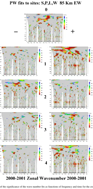
A unique analysis has been developed to establish the wave numbers of the complete spectrum of oscillations avail-able from the wavelet analysis, as applied to the set of ob-serving sites (Fig. 4). The model restricts the waves to E-W propagation, and the positive wave number m is for the west-ward direction. For each value of m (0, +/−1, +/−2, etc.), and each frequency, the minimum error for the fit between the phase-observations for the site and the wave model (a function of phase (longitude), wave number, and wave fre-quency) is calculated. Figures resulting from such calcula-tions can be annual contours of “normalized” squared error

(range 0–1) intensities as functions of frequency and time for wave numbers from 0 to +/−4. However, since the signif-icance of a given fit-error value depends on the number of sites used, fit-errors for the radar data are translated into sig-nificance levels by comparison, with errors obtained using randomly distributed test data. Significances (88–100%) are, therefore, plotted. Finally in this sequence of analyses (Fig-ure 5a, b), contour plots of frequency versus time for a given subset of the radars have also been prepared to indicate the preferred wave number (based upon the mode with minimum fit-error) at the given level of statistical significance (95%). There is also the potential for aliasing, and this matter is dis-cussed later.

For the comparisons of PW activity at the CUJO sites (Sect. 4) an independent planetary wave (PW) analysis is done for selected frequencies, starting with a year of hourly mean data which is extended at the ends, if data are avail-able, to accommodate the desired window length. For the 16 day period, a 48-day window length, and for 2-day peri-ods, a 24-day window, are each shifted in 5-day steps over the year. For each of these window-lengths the mean is re-moved and used to represent the background wind, and then a full cosine window (Hanning) is applied and the Fourier transform is done at the single selected PW frequency. With (cosine) windowing the window lengths are effectively re-duced to about half of the stated lengths and side-lobes are minimized; the bandwidths are then 12–24 and 1.8–2.2 days, respectively, which cover the normal range of periods consid-ered for these waves in the MLT region. Gaps are not filled. Annual contours of wave amplitudes as functions of height versus time are then prepared for each wind component and radar-location (Figs. 6, 7). It is possible that trends in the background winds during the equinox months could contam-inate the amplitudes of the 16-day PW, but the contour plots discussed later show no indication of this; meanwhile, the Fourier transforms are more robust with optimized numbers of degrees of freedom.

The following data rejection criteria apply to both this analysis and to the earlier wavelet analysis. The spectral val-ues are accepted if at least 80% of the phases for that wave are available from the windowed data in each of two sep-arate period intervals within the window, i.e. data must be available in 80% of the “phase-bins” in at least two separate cycles. Otherwise, the pixel is left white (data omitted). To facilitate the application of this criterion the phases are sub-divided into 24 bins; but in the case of the wavelet analysis for periods less than 24 h, the number of bins is equal to the period in hours. Note that this criterion is similar to the weaker one that we regularly use for tidal analysis (e.g. Man-son et al., 2002a), for which we require data in 16 different UT hours to be available.

This process is equivalent to a band-pass filter of 10–100 min for the GW variances, and has been discussed in some de-tail by Nakamura et al. (1993). The second is applied to hourly mean data (Gavrilov et al., 1995), and is equivalent to a band-pass filter of approximately 2–6 h (HD) for the GW variances.

Both the hourly difference (HD) and 5-min difference (5mD) filters use a centred 24-day interval shifted by 5 days for the contour plots. In the case of Wakkanai and Yama-gawa, where the original records are spaced by 2 min rather than 5 min, they are given a 5-min “index”. This means that the rms values at these sites are combinations of 4, 6 and 8 min differences. Also, since the record length for the FCA analysis is 2 min, the squared differences have been divided by 2.2 to match the wind variances of the other sites with record lengths of 4.5 min (Meek and Manson, 2001; Manson et al., 1999). For the HD data, in addition to the raw wind variance adjustment, each individual hourly difference is ad-justed based on the number of values in each hour, (which must be 3 or more, 7 for the ATRAD systems), to be equiv-alent to what would be expected if there were twelve 5-min values available in each hour. A minimum of 100 difference values per height and time “bin” is required for the HD and 5mD analyses before a value is plotted. For the background mean wind, each day used must have at least 8 h of data, and there must have been at least 6 days of the 24-day in-terval with such daily data. Although these means may not be the same as the tidally corrected means, for example in Figs. 6 and 7, they better reflect the background wind cor-responding to the measured HD and 5mD data. Once the sequences of GW variances from the two filters are available they have been organized as annual contours of GW ampli-tudes as functions of height versus time, for the zonal and meridional (EW, NS) components, and for each radar loca-tion (Figs. 8, 9).

3 Climatologies of atmospheric oscillations (5 h to

30 days) at the CUJO radars

3.1 Wavelet spectral intensities

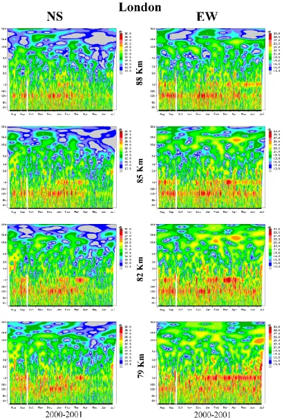
Preparations for the first paper on the CUJO radars (Manson et al., 2003), that included winds and ionospheric data from the Platteville and Saskatoon MFRs, illustrated the value of annual climatologies of the spectral content of the wind field. We use that presentation format here also. The use of the word climatology may be argued, since here we show one year of data; however, the spectral contour plots from previ-ous and subsequent years for the sites of CUJO are generally similar to those shown here. (A similar conclusion is reached for other types of seasonal plots shown in this paper.) The “wavelet” spectral analysis method was described in Sect. 2, and the resulting annual contours of wavelet intensities as functions of frequency and time for the London MFR are shown in Fig. 1. Both components of the wind (EW, zonal; NS, meridional) are shown for four heights (79–88 km).

The main purpose of Fig. 1 is to indicate the rather mod-est changes in contour characteristics throughout the height range. In both components and for all heights the semi-diurnal (12-h) and semi-diurnal (24-h) oscillations are clearly present throughout the year. For longer periods in the PW range, oscillations are much more evident in the EW compo-nent, although 2-day activity is also present in the NS. The other 4 MFRs also show modest changes in contours with height. Generally, differences between the CUJO locations discussed below are larger than over 3–5 km height ranges at individual locations.

Significance levels are relatively simple to provide but of-ten their calculation involves assumptions that are difficult to justify. For the spectra of Figs. 1 and 2 (below) vari-ous estimates (including Luo et al., 2002a, b) suggest that levels above 95% are above the 21-dB contour levels (circa 10 m/s), and that these usually exist for time intervals of a longer duration. However, for these global scale waves it can also be argued that a better indication of geophysical signifi-cance is their simultaneous presence at all sites of the CUJO network. Thus, Fig. 3, also discussed below, which provides the geometric means of wavelet intensities for the three 40-degree locations, has value in this regard. Annual contours of wavelet intensities for the five MFR locations are now pro-vided in Fig. 2. The middle altitude of 85/86 km is shown, as are EW and NS components. The highest latitude location (52◦N) is at the top, the three 40–45◦N locations in the mid-dle for easiest comparison, and the lowest latitude (31◦N) is at the bottom. The relative latitudinal variation of the two tides is clearly evident: at Yamagawa the 24-h tide domi-nates; at Wakkanai, Platteville and London the 12- and 24-h tidal intensities are quite comparable; while at Saskatoon the 12-h tide dominates. This latitudinal variation is consistent with earlier studies (e.g. Manson et al., 2002a; Pancheva et al.,2002).

Detailed comparisons of the tides at the 40-degree loca-tions will appear elsewhere (Thorsen, Private Communica-tion, 2002), where all available heights and tidal phases will be considered. However, even in Fig. 2, substantial differ-ences are apparent. Considering the contour levels of both components throughout the year, Platteville has the largest tides and the 12/24-h amplitudes are comparable, while Lon-don has the smallest amplitudes with smaller NS than EW components. The amplitudes at Wakkanai lie between the other two, but there, the 12-h tide is larger than the 24-h tide. Comparisons with the global HRDI-UARS tides (Manson et al., 2002b) are difficult for many reasons: they were at 96 km, during 1993/1994, and for selections of 2-monthly intervals that do not correspond to the time-resolution of Fig. 2. All that can be said is that the HRDI tides frequently evidence cells across both North America and the Pacific, whose am-plitude differences are 3–6 dB, and such differences can be seen in Fig. 2 as one scans along the monthly time axes for the three MFRs.

geomet-Fig. 1. Annual contours of wavelet intensities as functions of frequency and time for the zonal and meridional (EW, NS) components of the

Fig. 2. Annual contours of wavelet intensities as functions of frequency and time for the zonal and meridional (EW, NS) components of the

ric means of wavelet intensities at Wakkanai, Platteville and London. It is useful first to remind the reader of the observed oscillation-periods usually associated with the classical west-ward propagating Rossby “normal” PW modes (the so-called 5-, 10-, 16-day waves) and other PW oscillations, such as the quasi 2-d Rossby-gravity normal mode. The ranges of ob-served periods associated with these are typically 2, 5–7, 8– 10, 12–22 days, due to Doppler shifting by the background winds (Luo et al., 2002a, b). In addition, careful assessment of the low frequencies in such spectra has revealed the ad-ditional presence of oscillations of an “extra long period” (20–40 days) that have correlations with the solar rotation period (27-days) (Luo et al., 2001), and climatologies rather similar to the 16-day PW. Finally, there is some evidence that PW oscillations near a 5-day period, in particular the 7-day PW of 1993 (Clark et al., 2002), are on occasion unstable or are baroclinic modes excited in situ in the mesosphere.

Returning to Fig. 2 and the dominant zonal component, the contour maxima associated with the 16-day PW are very strong near periods of 12-14 days in the winter-centred months at Platteville (as they are to a lesser degree at Saska-toon), but are much weaker (3 dB) at London. The temporal variability is similar. However, at Wakkanai, there is com-paratively little activity (contours of low amplitude) in that band and much more in that of the “extra long period” oscil-lation (20–30 days). There is also comparatively little of that latter activity at the two other 40-degree locations, or at Ya-magawa. Saskatoon evidences both 16-day and ’long period’ activity at the same times.

It is not easy to spectrally distinguish the 10-d PW in such (zonal) spectra, and the authors are unaware of focussed stud-ies of this mode. Taking the nominal range as 8–10 days, Wakkanai has more activity than the other locations. The contour structures associated with the 5-d PW show consid-erable variability: activity is almost absent at London, but in-creasingly evident at Saskatoon and Wakkanai in both com-ponents. The occurrences are spread over a wider interval of time and include the equinoxes. This temporal and spatial intermittency may be a function of the unstable modes often associated with this frequency range.

The quasi-2-d PW is well represented in the contour max-ima (activity) at Saskatoon, Platteville and Wakkanai dur-ing summer months (July, August) but increasdur-ingly less so at London and Yamagawa. For this mode the NS compo-nent activity is comparable or larger to that for the EW (see also Fig. 3), as is well known (Thayaparan et al., 1997). The height of 85 km was carefully chosen so that PW ac-tivity from 2–30 days would be well represented, for exam-ple, although 16-d PW activity is known to exist throughout the MLT in winter, it is limited sporadically to heights near 85 km in summer months (Luo et al., 2002a, b). In this con-text, the summer mesopause activity for the 2-d PW is well studied, but here in Fig. 2 there is considerable winter activ-ity at all locations. Specific 2-d and 16-d height-time contour plots will be presented and discussed later in Sect. 4.

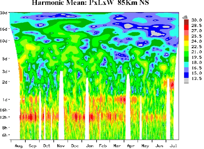
Finally, the plots of annual contours that are (geometric) means of the wavelet intensities for the three 40-degree

lo-cations (Fig. 3) form a useful summary of wave activity. In the zonal plot, the activity for the “long period” oscillations, and for 16-d and 2-d PWs, is very clear. The 5- to 7-d and 10-d PW activity is very weak. The meridional plot also shows minimal activity for periods greater than 5 days, con-sistent with the polarization of the waves (Luo et al., 2002a). Tidal activity must be considered in the context of its strength throughout the MLT, but at 85 km and for both components, the 12 h demonstrates the well-known winter and equinox maxima (especially the early autumn), and the 24 h has win-ter and spring maxima. As the detailed Platteville- Saskatoon comparison showed (Manson et al., 2003), the equinoctial dominance of the equatorial and sub-tropical 24-h tide is not yet established at 40–45 degrees. Comparisons of Figs. 2 and 3 indicate variability or intermittency of wave activity across the CUJO network; bursts of significant activity do occur at different times across the region, and as noted by Luo et al. (2002a, b), this makes it difficult to assign wave numbers to the spectral components.

3.2 Wave numbers for CUJO spectral intensities

The use of the wavelet spectral intensities for the CUJO net-work of MFR locations was described in Sect. 2. The annual contours of the significance of the respective wave number fits as functions of frequency and time for the EW compo-nent and for wave numbers from 0 to±4 are provided in Fig. 4. Largest numbers (99–100%, red colour band) indi-cate the best fitting between the wave number model and the data from the 4 middle latitude MFRs, and indicate the (%) chance the fit did not occur randomly. Other combinations of stations were included in this analysis, for example, Yam-agawa and even a European location, but no improvements in consistency of the contour characteristics were obtained. The wave characteristics do change toward 31◦N (Sect. 3.1, Fig. 2), and that along with PW intermittency (Luo et al., 2000b), do not support the use of either the low latitude or a distant European location.

The significance of a fit depends on the measured least-squares error and the expected distribution of these fit-errors when the site-phases are random. These distributions, generated from sets of random phases, were found to depend on the number of sites, but not their longitude locations or on the mode fitted. On the other hand, there can be mode-ambiguity depending on the set of locations. For example, if we have 2 sites separated by exactly 120 degrees of lon-gitude, there is no way to distinguish between mode 0 and mode 3, since the phases are the same at both sites for both these modes. This also applies to any 2 modes separated by +/−3, for example, m=−1 and m=2, or m=1 and m=4, etc. It was shown that the above arguments apply to some extent to the present sites, since they are in two groups separated by

Fig. 3. Annual contours of wavelet intensities as functions of frequency and time for the zonal and meridional (EW, NS) component of the

wind. The geometric means of intensities from three locations (London, Platteville, Wakkanai) are shown for the altitude of 85/86 km.

the squared differences between the fit-errors for each pair of modes were accumulated. Aliasing is more likely in mode-pairs when such differences are small. As expected for our site-distribution this was found to apply to mode-pairs whose wave numbers differ by +/−3.

The wave numbers for the tides will be part of a deeper discussion of tides elsewhere (Thorsen, Private Communi-cation, 2002). We use them here as a test of the analysis.

the contours are of the preferred wave number (smallest fit-error) for each frequency versus time pixel, where colours are only shown when this error is at the 95% significance level compared with random sets of phases. Three altitudes have been included here (82–88km) to improve the statistical sta-bility, which translates into colour consistency, at this 95% level. As expected from Fig. 4, the late-winter/spring inter-val is dominated by the dark green (m=1) and silver (m=4) areas. Otherwise, blue (m=3, or 2) is quite common. An al-ternative presentation is provided in Fig. 5b: here, the wave numbers of Fig. 5a are folded into just m=0, 1, 2, fully allow-ing for the possibility that aliasallow-ing and statistical couplallow-ing of mode-pairs, whose wave numbers differ by +/−3, have dom-inated the analysis. Thus, in this extreme case of Fig. 5b, m=1 (green) is dominant, with modest regions of m=0 (red) and 2 (blue).

For the 12-h tide the m=2 component is the clear favourite from Fig. 4, with the red/orange areas of high significance (small “fit-errors”) being dominant, especially when the tide is large in the equinoxes and winter (Fig. 3). There are also some time intervals when m=0, where 3 have high sig-nificances. The tide with a higher statistical probability of aliasing (m=−1) is again not favoured. The contours of the preferred wave number (95% significance) in Fig. 5a show a clear dominance of the pale-blue areas (m=2) with some dark-blue (m=3) and dark-green (m=1). The extreme case of Fig. 5b shows m=2 (blue) to still dominate, with m=0 (red) replacing the m=3, and some m=1 (green) remaining.

The published studies of non-migrating (solar) tides or components offer useful comparisons with these results. Forbes et al. (2003) used 95-km HRDI observations of the 24-h tide and mention the m=0, 2 and 3 tides for latitudes below 40◦_{(we noted m=2, 3, 4 in Fig. 5a, and m=0, 2 in the}

extreme case of Fig. 5b). Angelats i Coll and Forbes (2002) mention m=1 and 3 for the 12-h tide as the result of interac-tions with the standing m=1 PW (we noted m=1, 3 in Fig. 5a, and m=0, 1 in the extreme case of Fig. 5b). There are indi-cations of agreement, but more stations at useful positions in Europe or Asia are needed to reduce the uncertainties due to aliasing. The value of the extreme case of Fig. 5b, which ig-nores the individual wave numbers having 95% significance levels and assumes the worst case of aliasing, is rather mixed: for the 24-h tide, it improves the dominance of the m=1 mi-grating tide and improves agreement with the HRDI observa-tions for the non-migrating tides; while for the 12-h tide the agreement with the HRDI observations is not improved.

We now consider the PW modes in Figs. 4 and 5. The m=1 mode has the largest areas of red-yellow (high significances, small “fit-errors”) for periods from near 10-days to 30-days in Fig. 4, and they are in winter months when the PW ampli-tudes are largest (Fig. 3). The other modes with somewhat smaller areas of red-yellow included m=−2, 4 (the modes of highest potential aliasing), and m=0, 3. The favoured modes near the quasi-2-d PW are less distinct, with m=3 and 4 being weakly favoured.

Consistent with that, the contours of statistically (95%) preferred wave numbers in Fig. 5 show a dominance of

dark-green (m=1) for periods of 10–30 days in winter months, al-though dark-blue and silver areas (m=3 and 4) are also evi-dent (Fig. 5a), or m=0 (red) for the extreme case (Fig. 5b). More specifically, modes favoured at times of maximum am-plitude, i.e. December, February and April/May in Fig. 3, are first m=1 and then m=3 (Fig. 5a) or 0 (Fig. 5b). The pre-ferred wave numbers near the 2-d PW in Fig. 5a are m=4 and 3 (silver and dark blue) in the summer, with other modes such as m=2 (pale blue) appearing in the winter. The ex-treme (aliasing, coupling) case of Fig. 5b (and indeed CUJO itself) is not ideal for the 2-d PW, as it enhances the m=1 (green) areas at the expense of m=4, and replaces the m=3 with m=0 (red). Wave number contour plots that included the low latitude location (Yamagawa) provided similar PW contour characteristics to Fig. 5, but the high significance ar-eas were often smaller. This is consistent with differences in the wavelet intensity contours of Fig. 2.

The wave number which is theoretically and observation-ally usuobservation-ally associated with the 5, 10 and 16-d PWs is m=1 (e.g. Forbes et al., 1995; Luo et al., 2002a). However, the latter paper noted the variability and intermittency of the 16-d PW, both spatially and temporally, which often leads to considerable difficulty in associating clear wave numbers with a burst of PW activity. We also note that CUJO is not a global network, and these wave number fits refer to a global segment of 7 000 km. Finally, the wave numbers for the 2-d PW that are theoretically and observationally preferred from earlier studies (e.g. Thayaparan et al., 1997; Meek et al., 1996), range from 3–5, with a preference for m=3. How-ever, there is also evidence that unstable modes exist near this period (e.g. Plumb, 1983), and the less well-studied win-ter manifestations of the 2-d PW may well have other wave number values (see below).

4 Climatologies of 16-d, 2-d PW

4.1 16-d PW

The annual contours of wave amplitudes as functions of height versus time for EW and NS components of the winds over the CUJO network are shown in Fig. 6. The background-mean winds (BGW) for the 48-day window (Sect. 2.2) are also shown. The relative amplitudes within the MLT and across CUJO are consistent with the spec-tra of Fig. 2: the EW amplitudes are dominant; London and Yamagawa have the smallest amplitudes; the wave ac-tivity (amplitudes above 5 m/s) is largest in winter-centred months; and the wave activity is restricted to mesopause heights (∼80 km) in summer. Significance levels, as in Luo et al. (2002a, b), are 90–95% for the gray scale regions hav-ing amplitudes of 5–9 m/s.

Fig. 4. Annual contours of the significance of the wave number fits as functions of frequency and time for the zonal (EW) component of the

wind and for wave numbers from 0 to +/−4: the altitude is 85/86 km. Largest numbers (99–100%) indicate best fitting between the wave

Fig. 5. Annual contours of the preferred wave number (at the 95% significance level) as functions of frequency and time for the zonal (EW)

component of the wind and for the 4 locations of Fig. 4. The data from 3 heights (82, 85, 88 km) are used for added statistical stability. In

0 5 9 13 Amplitude (m/s)

Saskatoon (52N,107W) 2000-2001 EW 16-d & BGW

Aug Sep Oct Nov Dec Jan Feb Mar Apr May Jun Jul 70 75 80 85 90 95 Height (km) 10 10 10 -20 -40 -30 -20 -30

Saskatoon (52N,107W) 2000-2001 NS 16-d & BGW

Aug Sep Oct Nov Dec Jan Feb Mar Apr May Jun Jul 70 75 80 85 90 95 5 5 5 5 5 0 5 9 13 Amplitude (m/s)

Platteville (40N,105W) 2000-2001 EW 16-d & BGW

Aug Sep Oct Nov Dec Jan Feb Mar Apr May Jun Jul 70 75 80 85 90 95 Height (km) 10 10 10 -30 -20

Platteville (40N,105W) 2000-2001 NS 16-d & BGW

Aug Sep Oct Nov Dec Jan Feb Mar Apr May Jun Jul 70 75 80 85 90 95 5 5 5 0 5 9 13 Amplitude (m/s)

London (43N,81W) 2000-2001 EW 16-d & BGW

Aug Sep Oct Nov Dec Jan Feb Mar Apr May Jun Jul 70 75 80 85 90 95 Height (km) 10 10 10

London (43N,81W) 2000-2001 NS 16-d & BGW

Aug Sep Oct Nov Dec Jan Feb Mar Apr May Jun Jul 70 75 80 85 90 95 0 5 9 13 Amplitude (m/s)

Wakkanai (45N,141E) 2000-2001 EW 16-d & BGW

Aug Sep Oct Nov Dec Jan Feb Mar Apr May Jun Jul 70 75 80 85 90 95 Height (km) 10 10 10 -30-20

Wakkanai (45N,141E) 2000-2001 NS 16-d & BGW

Aug Sep Oct Nov Dec Jan Feb Mar Apr May Jun Jul 70 75 80 85 90 95 5 5 0 5 9 13 Amplitude (m/s)

Yamagawa (31N,130E) 2000-2001 EW 16-d & BGW

Aug Sep Oct Nov Dec Jan Feb Mar Apr May Jun Jul 70 75 80 85 90 95 Height (km) 10 10 10 10 -30 -20

Yamagawa (31N,130E) 2000-2001 NS 16-d & BGW

Aug Sep Oct Nov Dec Jan Feb Mar Apr May Jun Jul 70 75 80 85 90 95 5 5 5

Fig. 6. Annual contours of wave amplitudes as functions of height versus time for the zonal and meridional (EW, NS) components of the 16-d

consistent with the high significance of the m=1 wave mode discussed earlier (Fig. 4) at these times, which requires co-herence of the oscillation in space and time. Nevertheless, the variation of wave activity and amplitudes with longitude is quite substantial in winter and summer months, with Plat-teville and Saskatoon (very similar longitudes) being quite similar in the winter months.

The recent studies of this wave (Luo et al., 2002a, b) noted its spatial and temporal intermittency, with bursts of activity occurring at different times at the MFR locations: Tromsø (70◦N, 19◦E), Saskatoon (52◦N, 107◦W), London (43◦N, 81◦W), Hawaii (22◦N, 159◦E), Christmas Island (2◦N, 157◦E). Although four of these radars are from the Pacific-North American sector, the range of latitudes and lon-gitudes is now seen to be very considerable. Also, results from the UARS-HRDI system (Luo et al., 2002b), which are based upon hemispheric wave mode (m=1) fits, showed strong latitudinal restrictions or spatial intermittency in the bursts of activity. The new results here indicate that while longitudinal coherency may exist during bursts of wave ac-tivity (based upon the mode fitting at significant levels), the overall longitudinal variability of amplitudes at particular lat-itudes (40–45◦N) is often comparable with the latitudinal variations.

These issues of intermittency, and of varying period for the 16-d PW (Fig. 2), were thoroughly explored in the above papers and will not be repeated here at any length. The the-oretical expectation for this wave is for propagation from the lower atmosphere and resulting activity throughout the win-ter hemisphere’s eastward flow, with the possibility of sum-mer mesopause activity due to propagation from the winter hemisphere. The results from the 2-D Global Scale Wave Model (GSWM) in Luo et al., (2000, 2002b) were generally consistent with this simple scenario, but also demonstrated strong sensitivity to the background winds in the model. Our observations reinforce those conclusions: we again hypothe-size that local conditions (winds, other PW modes, PW and GW interactions, and temperatures) may favour responses or resonances of different amplitude and at different periods at different sites. Detailed 3-D modelling is needed to assess these effects.

Finally, we note that interannual variability for the 16-d PW is considerable (Luo et al., 2000), so that the results of wave studies from other years are expected to show some differences from Fig. 6. However, some differences be-tween certain locations will persist; wave activity at London and Saskatoon for 1995 also showed similar relative contour structures (amplitudes, heights) to 2000–2001.

4.2 2-d PW

The annual contours of wave amplitudes for the 2-d PW are shown in Fig. 7; the same format as Fig. 6 has been used. Despite the considerable number of studies of this wave type over the last two decades (e.g. Meek et al., 1996; Thayaparan et al., 1997), contour plots of this type are still quite rare. In-deed most emphasis has been on the bursts of activity during

summer months (July–August in the Northern Hemisphere) at mesopause heights. One reason for this is the early use of simple meteor radars without height ranging, which provided almost exclusively mesopause data.

In that context we note the strong summer mesopause ac-tivity (amplitudes above 5 m/s, and significance levels above 90%) in both the EW and NS components at Saskatoon, Plat-teville and Wakkanai. Again the Yamagawa and particu-larly the London activity and amplitudes are quite small. Of greater note, however, is the winter activity that can be seen throughout the MLT at all stations, except at London. Con-sidering the London data, the background winds of winter are comparable to those elsewhere in CUJO, so there is no evidence for a bias in the winds-analysis there. Indeed the Meek (1980) and Briggs (1984) styles of analysis have both been used there at the time of establishment of the radar, and no significance differences were found (Thayaparan et al., 1995). The 2-d PW activity at Yamagawa demonstrates the expected sub-tropical behavour, with maxima in both sol-stices, consistent with wave propagation from the Southern Hemisphere in one solstice. The NS component is also dom-inant there.

The longitudinal variability of wave activity is again con-siderable for the three 40-degree stations, with the stations of close to common longitude (Saskatoon and Platteville) being much more similar in activity and structure. The bursts of wave activity are close to simultaneous in summer, but less so in winter. Notice that the geometric means of Fig. 3 do show strong (>24 m/s) contours in both solstices, and it is only at these times that the wave is consistently evident at all longi-tudes near the 40-degrees latitude. In this regard the spatial coherence of this wave appears lower than for the 16-d PW, as the favoured wave numbers of Figs. 4 and 5 (m=3, 4 in summer, m=2, 3 in winter) were much less clear and consis-tent.

4.3 Theory and modelling

The theoretical underpinning for the 2-d PW has followed a similar path to that of the 16-d PW, so some discussion is warranted here. Salby (1981) provided the first quantita-tive treatment, and demonstrated that propagation of the 2-d wave (m=3) was favoured by a mean flow modestly eastward of the westward propagating wave (summer); and propaga-tion of the 16-d wave (m=1) was favoured within the winter’s eastward flow. This work was significantly developed by Ha-gan et al. (1993), who used their 2-D GSWM in the January solstice, and with three global mean wind fields, to investi-gate the 2-d PW (m=3 mode) propagation behaviour. It is useful to interpret the PW propagation in the context of the refractive index for PW developed by Charney and Drazin (1961), modifying that only to include the intrinsic frequency of a propagating wave, rather than the standing waves which were their focus (Luo, 2002).

0 5 7 9 Amplitude (m/s)

Saskatoon (52N,107W) 2000-2001 EW 2-d & BGW

Aug Sep Oct Nov Dec Jan Feb Mar Apr May Jun Jul 70 75 80 85 90 95 Height (km) 10 10 10 10 -40 -30-20 -40 -30 -20

Saskatoon (52N,107W) 2000-2001 NS 2-d & BGW

Aug Sep Oct Nov Dec Jan Feb Mar Apr May Jun Jul 70 75 80 85 90 95 5 5

5 5 5 5

5 0 5 7 9 Amplitude (m/s)

Platteville (40N,105W) 2000-2001 EW 2-d & BGW

Aug Sep Oct Nov Dec Jan Feb Mar Apr May Jun Jul 70 75 80 85 90 95 Height (km) 10 10

Platteville (40N,105W) 2000-2001 NS 2-d & BGW

Aug Sep Oct Nov Dec Jan Feb Mar Apr May Jun Jul 70 75 80 85 90 95 5 5 5

5 5 5

5 0 6 8 10 Amplitude (m/s)

London (43N,81W) 2000-2001 EW 2-d & BGW

Aug Sep Oct Nov Dec Jan Feb Mar Apr May Jun Jul 70 75 80 85 90 95 Height (km) 10 10 10

London (43N,81W) 2000-2001 NS 2-d & BGW

Aug Sep Oct Nov Dec Jan Feb Mar Apr May Jun Jul 70 75 80 85 90 95 0 6 8 10 Amplitude (m/s)

Wakkanai (45N,141E) 2000-2001 EW 2-d & BGW

Aug Sep Oct Nov Dec Jan Feb Mar Apr May Jun Jul 70 75 80 85 90 95 Height (km) 10 10 10 -40 -20

Wakkanai (45N,141E) 2000-2001 NS 2-d & BGW

Aug Sep Oct Nov Dec Jan Feb Mar Apr May Jun Jul 70 75 80 85 90 95 5 5 5 -15 -10 0 6 9 12 Amplitude (m/s)

Yamagawa (31N,130E) 2000-2001 EW 2-d & BGW

Aug Sep Oct Nov Dec Jan Feb Mar Apr May Jun Jul 70 75 80 85 90 95 Height (km) 10 10 10 10

Yamagawa (31N,130E) 2000-2001 NS 2-d & BGW

Aug Sep Oct Nov Dec Jan Feb Mar Apr May Jun Jul 70 75 80 85 90 95 5 5 -10

Fig. 7. Annual contours of wave amplitudes as functions of height versus time for the zonal and meridional (EW, NS) components of the 2-d

of a critical level (zero intrinsic phase speed); such levels are experienced by this rather slowly moving wave in the summer’s strong westward flow. In contrast, the faster mov-ing (m=3) 2-d wave escapes this fate and achieves signifi-cant summer amplitudes (Hagan et al., 1993, Figs. 2, 4, 6) at mesopause heights (85–90 km) and even at middle lati-tudes (the CUJO range). (Maximum responses are between the equator and±30◦.)

In winter the eastward flow leads to larger intrinsic phase speeds, but the so-called “critical velocity” (Charney and Drazin, 1961; Luo, 2002) is often not exceeded by the 16-day wave, and large amplitudes may be achieved through-out the MLT. This is consistent with observations here and elsewhere, and also the GSWM results in Luo et al. (2002). However, the “critical velocity”, which is a function of both phase speed and wave number (m=3), is smaller for the 2-d wave and rather easily exceeded during the winter months. Hence, the amplitudes of this wave are expected to be smaller in winter, as Hagan et al. (1993) demonstrate. This modest solstitial difference in the GSWM‘s response may have been overstated, however, by interpreters of this paper, as the results here (and at the Tromsø MFR, Nozawa et al., 2003) show substantial winter amplitudes.

With regard to the topic of intermittency, we note that Ha-gan et al. (1993) very nicely address this issue, which is a clear feature of the 2-d PW (and of the 16-d PW, as we have demonstrated). They note that variations of the relative mag-nitudes of the summer and winter “jets” on time scales of weeks could account for the intermittency of the PW, and that the resonant period of the wave is sensitive to these changes in the “jets”. Such effects would be associated with the prop-agation of both 16- and 2-d PWs. Another aspect of this issue may involve the amplification of the quasi-2-d wave due to the interaction of that normal mode with the “generally un-stable mean (zonal) flow” (Salby and Callaghan, 2001). They demonstrate through modelling that this can lead to oscilla-tions of similar period (2.0–2.2 days) and with most likely wave numbers of 3 and 4; these should exist in summer and winter hemispheres, and would exhibit there what we have termed as intermittency.

Finally, as discussed by Salby (1981), the second Rossby gravity mode (m=2) could also be present in the MLT with significant amplitudes. While the range of periods for the m=3 mode could be confined to 1.9–2.5 days, the m=2 could be in the range of 1.6–1.9 days. The “critical velocity” for this mode is higher, which is consistent with significant win-ter amplitudes (Salby, 1981, Fig. 9), as observed here. We also note that the m=2 wave number occurred more fre-quently in the “preferred wave number” contours of Fig. 5 during winter, and that the spectral contours (Fig. 3) cover the range from 1.6–2.5 days.

5 Climatologies of gravity waves

In this brief section we show annual contours (climatolo-gies) of wave amplitudes for GWs in the 10–100 min and

2–6 h bands. Such climatologies were first shown by Meek et al. (1985) for data from the Saskatoon MFR, and we have since used that format frequently for that location. Subse-quent studies (e.g. Manson et al., 1999), have considered lat-itudinal variations, but this is the first longlat-itudinal assessment of GW variabilities.

The wind variances in the 10–100 min band are shown in Fig. 8, where climatologies from all five CUJO locations are provided, for EW and NS components. The background wind (Sect. 2.2) is also plotted, since it again dominates the propagation of the waves. A familiar semiannual oscillation is clear at Saskatoon in the EW component, with maxima during the solstices, at heights up to 90 km (readers famil-iar with earlier contour plots from this site should note that all of those used lines of constant intensity with a rather fine scale, rather than a broader “gray scale”, and that changes the “shape” of variations somewhat). Such SAO variations are well known and often incorporated in models such as the GSWM (e.g. Garcia and Solomon, 1985). Physically, the intrinsic phase velocities of GW maximize during the sol-stices due to the middle atmosphere “jets”, and once sat-urated, their perturbation speeds vary as that phase veloc-ity (Fritts, 1989); even NS components may be thus modu-lated, as all but purely NS propagating GW will experience Doppler shifting due to their components of the EW winds.

Of the other CUJO radars, London and Yamagawa were part of the previous study (Manson et al., 1999), and again the zonal GW variances at 43◦N show a clear SAO, while the 31◦N location has a much weaker one (below 77 km). Yama-gawa also has a winter maximum above 88 km. However, the variation of variances at Wakkanai is very similar to Yama-gawa, again showing that longitude changes (e.g. 5500 km from Saskatoon-Platteville) are more important than latitude changes (here, circa 1500 km). Platteville has similar vari-ance levels to Saskatoon, except during summer, when it shows only a very modest summer maximum. There is over-all a weaker tendency for the NS variances to have a SAO over the CUJO network.

The variances at London in this high frequency band are one complete gray-scale (4 m/s) higher than the other sites, consistent with the 1994 year of Manson et al. (1999). It has been suggested by Thayaparan et al. (1995), in the context of tidal variability, that the Great Lakes and associated weather may lead to higher regional GW fluxes.

Finally, we consider the GW climatologies for the 2–6 h band of associated wind variances (Fig. 9). In this format of gray scales the contours at Saskatoon and Platteville are very similar, with a strong SAO; London is very similar to 105–107◦W below 90 km (as for the 1994 study); and both Wakkanai and Yamagawa have a SAO and locally similar contours. The NS variances are less regular, with both SAO and AO being evident.

0 10 14 18 Amplitude (m/s)

Saskatoon (52N,107W) 2000-2001 EW Day:10-100min & BGW

Aug Sep Oct Nov Dec Jan Feb Mar Apr May Jun Jul 70 75 80 85 90 95 Height (km) 10 10 10 10 -20 -40-30 -20 -40 -30 -50

Saskatoon (52N,107W) 2000-2001 NS Day:10-100min & BGW

Aug Sep Oct Nov Dec Jan Feb Mar Apr May Jun Jul 70 75 80 85 90 95 5 5 5 5 5 5 0 10 14 18 Amplitude (m/s)

Platteville (40N,105W) 2000-2001 EW Day:10-100min & BGW

Aug Sep Oct Nov Dec Jan Feb Mar Apr May Jun Jul 70 75 80 85 90 95 Height (km) 10 10 10 -30 -20

Platteville (40N,105W) 2000-2001 NS Day:10-100min & BGW

Aug Sep Oct Nov Dec Jan Feb Mar Apr May Jun Jul 70 75 80 85 90 95 5 5 5 5 5 0 10 14 18 Amplitude (m/s)

London (43N,81W) 2000-2001 EW Day:10-100min & BGW

Aug Sep Oct Nov Dec Jan Feb Mar Apr May Jun Jul 70 75 80 85 90 95 Height (km) 10 10 10 10

London (43N,81W) 2000-2001 NS Day:10-100min & BGW

Aug Sep Oct Nov Dec Jan Feb Mar Apr May Jun Jul 70 75 80 85 90 95 0 10 14 18 Amplitude (m/s)

Wakkanai (45N,141E) 2000-2001 EW Day:10-100min & BGW

Aug Sep Oct Nov Dec Jan Feb Mar Apr May Jun Jul 70 75 80 85 90 95 Height (km) 10 10 10 10 -30 -20 -40 -20

Wakkanai (45N,141E) 2000-2001 NS Day:10-100min & BGW

Aug Sep Oct Nov Dec Jan Feb Mar Apr May Jun Jul 70 75 80 85 90 95

5 5 5

5 -15 -10 0 10 14 18 Amplitude (m/s)

Yamagawa (31N,130E) 2000-2001 EW Day:10-100min & BGW

Aug Sep Oct Nov Dec Jan Feb Mar Apr May Jun Jul 70 75 80 85 90 95 Height (km) 10 10 10 10 -30 -20

Yamagawa (31N,130E) 2000-2001 NS Day:10-100min & BGW

Aug Sep Oct Nov Dec Jan Feb Mar Apr May Jun Jul 70 75 80 85 90 95 5 5 5 5 -10

Fig. 8. Annual contours of wave amplitudes as functions of height versus time for the zonal and meridional (EW, NS) components of GWs

0 10 14 18 Amplitude (m/s)

Saskatoon (52N,107W) 2000-2001 EW 2-6h & BGW

Aug Sep Oct Nov Dec Jan Feb Mar Apr May Jun Jul 70 75 80 85 90 95 Height (km) 10 10 10 10 -20 -40 -30 -20 -40 -30 -50

Saskatoon (52N,107W) 2000-2001 NS 2-6h & BGW

Aug Sep Oct Nov Dec Jan Feb Mar Apr May Jun Jul 70 75 80 85 90 95 5 5 5 5 5 5 5 0 10 14 18 Amplitude (m/s)

Platteville (40N,105W) 2000-2001 EW 2-6h & BGW

Aug Sep Oct Nov Dec Jan Feb Mar Apr May Jun Jul 70 75 80 85 90 95 Height (km) 10 10 10 -30 -20

Platteville (40N,105W) 2000-2001 NS 2-6h & BGW

Aug Sep Oct Nov Dec Jan Feb Mar Apr May Jun Jul 70 75 80 85 90 95 5 5 5 5 5 5 5 0 10 14 18 Amplitude (m/s)

London (43N,81W) 2000-2001 EW 2-6h & BGW

Aug Sep Oct Nov Dec Jan Feb Mar Apr May Jun Jul 70 75 80 85 90 95 Height (km) 10 10 10

London (43N,81W) 2000-2001 NS 2-6h & BGW

Aug Sep Oct Nov Dec Jan Feb Mar Apr May Jun Jul 70 75 80 85 90 95 0 10 14 18 Amplitude (m/s)

Wakkanai (45N,141E) 2000-2001 EW 2-6h & BGW

Aug Sep Oct Nov Dec Jan Feb Mar Apr May Jun Jul 70 75 80 85 90 95 Height (km) 10 10 10 10 -30-20 -40 -20

Wakkanai (45N,141E) 2000-2001 NS 2-6h & BGW

Aug Sep Oct Nov Dec Jan Feb Mar Apr May Jun Jul 70 75 80 85 90 95 5 5 5 5 -15 -10 0 10 14 18 Amplitude (m/s)

Yamagawa (31N,130E) 2000-2001 EW 2-6h & BGW

Aug Sep Oct Nov Dec Jan Feb Mar Apr May Jun Jul 70 75 80 85 90 95 Height (km) 10 10 10 10 -30 -20

Yamagawa (31N,130E) 2000-2001 NS 2-6h & BGW

Aug Sep Oct Nov Dec Jan Feb Mar Apr May Jun Jul 70 75 80 85 90 95 5 5 5 -10

Fig. 9. Annual contours of wave amplitudes as functions of height versus time for the zonal and meridional (EW, NS) components of GWs

wave types, GWs will also have source variations associ-ated with topographic and climatological (troposphere) vari-ations. Comparisons between GW variances from 3-D mod-els, and observations such as these, are valuable as a means of confirming physical processes within these models (e.g. Manson et al., 2002c).

6 Comments

These will be brief, since each section has dealt with the wave type and the interpretation of data in some detail. This is the first study of such a comprehensive spectral nature that has compared annual spectra and contour plots of specific harmonics (planetary waves and gravity waves) from 3 radars of identical type at effectively constant latitude (40–45◦N) and longitudinal separations of 1 100, 5 500 and 7 000 km. Two of the radars had a neighbour distant by 12–14◦of lat-itude. Generally, the longitudinal variations in PW and GW activity and amplitudes are significant and often larger than the variations with latitude of two of the pairs. While longi-tudinal variations in tides are expected due to non-migrating (solar) components, and in GW due to regional wave inter-actions and sources, the variations in PW activity and ampli-tudes are more surprising. However the intermittency in time and space of the PW (16-day, 2-day) noted across CUJO is entirely consistent with earlier studies of these waves. While described in classical theory by global modes, it is clear that regional effects on the response of the atmosphere to PWs are considerable.

Acknowledgements. The Canadian authors mention with thanks the support of the NSERC Granting Agency, the University of Saskatchewan through ISAS, and the University of Western On-tario. The U.S. authors wish to acknowledge the support of the NSF grant ATM-9724570 to the University of Colorado.

Topical Editor U.-P. Hoppe thanks Y. Portnyagin for his help in evaluating this paper.

References

Angelats i Coll, M. and Forbes, J. M.: Nonlinear interactions in the upper atmosphere: The s=1 and s=3 nonmigrating semidiurnal tides, J. Geophys. Res., 107, A8, 10.1029/2001JA900179, 2002. Briggs, B. H.: The analysis of spaced sensor records by correlation techniques, in: Handbook for MAP, Vol. 13. SCOSTEP Secr., University of Illinois, Urbana, pp. 166–186, 1984.

Charney, J. G. and Drazin, P. G.: Propagation of planetary-scale disturbances from lower into the upper atmosphere, J. Geophys. Res., 66, 83–109, 1961.

Clark, R. R., Burrage, M. D., Franke, S. J., Manson, A. H., Meek, C. E., Mitchell, N. J., and Muller, H. G.: Observations of 7-d plane-tary waves with MLT radars and the UARS-HRDI instrument, J. Atmos. Sol. Terr. Phys. 64, 1217–1228, 2002.

Forbes, J. M., Hagan, M. E., Miyahara, S., Vial, F., Manson, A. H., Meek, C. E., and Portnyagin, Y. I.: Quasi-16 day oscillation in the mesosphere and lower thermosphere, J. Geophys. Res., 100, 9149–9163, 1995.

Forbes, J. M., Hagan, M. E., Zhang, X., and Hamilton, K.: Up-per atmosphere tidal oscillations due to latent heat release in the tropical troposphere, Ann. Geophysicae 15, 1165–1175, 1997. Forbes, J. M., Zhang, X., and Hagan, M. E.: Simulations of

di-urnal tides due to tropospheric heating from the NCEP/ NCAR Reanalysis Project, Geophys. Res. Lett., 28, 3851–3854, 2001. Forbes, J. M., Zhang, X., Talaat, E. R., and Ward, W.: Nonmigrating

Diurnal Tides in the Thermosphere, J. Geophys. Res., 108, A1, 10.1029/2002JA009262, 2003.

Fritts, D. C.: A review of gravity wave saturation processes, effects, and variability in the middle atmosphere, Pure Appl. Geophys. 130, 343–371, 1989.

Garcia, R. R. and Solomon, S.: The effect of breaking gravity waves on the dynamics and chemical composition of the mesosphere and lower thermosphere, J. Geophys. Res., 90, 3850–3868, 1985. Gavrilov, N. W., Manson, A. H., and Meek, C. E.: Climatologi-cal monthly characteristics of middle atmosphere gravity waves (10 min–10 hrs.) during 1979–1993 at Saskatoon, Ann. Geophys-icae 13, 285–295, 1995.

Hagan, M. E., Forbes, J. M., and Vial, F.: Numerical Investiga-tion of the PropagaInvestiga-tion of the Quasi 2-Day Wave into the Lower Thermosphere, J. Geophys. Res. 98, 23 193–23 205, 1993. Hagan, M. E. and Roble, R. G.: Modeling diurnal tidal variability

with the NCAR TIME- GCM, J. Geophys. Res. 106, 24 869– 24 882, 2001.

Hocking, W. K. and Thayaparan, T.: Simultaneous and co-located observations of winds and tides by MF and meteor radars over London, Canada (43 N, 81 W) during 1994–1996, Radio Sci., 32, 833–865, 1997.

Igarashi, K, Nishimuta, Y., Murayama Y., Tsuda, T., Nakamura T., and Tsutsumi M.: Comparison of wind measurements between the Yamagawa MF radar and the MU radar, Geophys. Res. Lett., 23, 3341–3344, 1996.

Jacobi, Ch., Portnyagin, Y. I., Solovjova, T. V., Hoffmann, P., Singer, W., Fahrutdinova, A. N., Ishmuratov, R. A., Beard, A. G., Mitchell, N. J., Muller, H. G., Schminder, R., Kurschner, D., Manson, A. H., and Meek, C. E.: Climatology of the semidiurnal

tide at 52–56◦N from ground-based radar wind measurements

1985–1995, J. Atmos. Solar-Terr. Phys., 61, 975–991, 1999. Kumar, P., and Foufoula-Georgiou, E.: Wavelet analysis for

geo-physical applications, Rev. Geophysics, 35, 385–412, 1997. Luo, Y., Manson, A. H., Meek, C. E., Meyer, C. K., and Forbes, J.

M.: The quasi 16-day oscillations in the mesosphere and lower thermosphere at Saskatoon (52 N, 107 W), 1980–1996, J. Geo-phys. Res., 105, 2125–2138, 2000.

Luo, Y., Manson, A. H., Meek, C. E., Igarashi, K., and Jacobi, Ch.: Extra long period (20–40 day) oscillations in the mesospheric and lower thermospheric winds: observations in Canada, Europe and Japan, and considerations of possible solar influences, J. At-mos. Solar-Terr. Phys., 63, 835–852, 2001.

Luo, Y.: Influences of Planetary Waves upon the Dynamics of the Mesosphere and Lower Thermosphere, Ph.D. Thesis, 2002. Luo, Y., Manson, A. H., Meek, C. E., Thayaparan, T., MacDougall,

J., and Hocking, W.: The 16-day wave in the mesosphere and lower thermosphere: simultaneous observations at Saskatoon (52 N, 107 W) and London (43 N, 81 W), Canada, J. Atmos. Solar-Terr. Phys., 64, 1287–1307, 2002a.

the GSWM modeling results, Ann. Geophysicae, 20, 691–709, 2002b.

Manson, A. H., Meek, C. E., Brekke, A., and Moen, J.: Mesosphere and lower thermosphere (80–120 km) winds and tides from near Tromsø (70 N, 19 E): comparisons between radars (MF, EISCAT, VHF) and rockets, J. Atmos. Terr. Phys. 54, 927–950, 1992. Manson, A. H., Yi, F., Hall, C., and Meek, C. E.: Comparisons

between instantaneous wind measurements made at Saskatoon (52 N, 107 W) using the co-located medium frequency radars and Fabry-Perot interferometer instruments: climatologies (1988– 1992) and case studies, J. Geophys. Res. 101, 29 553–29 563, 1996.

Manson, A. H., Meek, C. E., and Zhan, Q.: Gravity wave spec-tra and direction statistics for the mesosphere as observed by MF radars in the Canadian Prairies (49 N–52 N) and at Tromsø (69 N), J. Atmos. Sol. Terr. Phys. 59, 993–1009, 1997.

Manson, A. H., Meek, C. E., Hall, C., Hocking, W. K., MacDougall, J., Franke, S., Igarashi, K., Riggin, D., Fritts, D. C., and Vincent, R. A.: Gravity wave spectra, directions and wave interactions: Global MLT-MFR network, Earth Planets Space 51, 543–562, 1999.

Manson, A. H., Meek, C. E., Hagan, M., Koshyk, J., Franke, S., Fritts, D., Hall, C., Hocking, W., Igarashi, K., MacDougall, J., Riggin, D., and Vincent, R.: Seasonal Variations of the Semi-Diurnal and Semi-Diurnal Tides in the MLT: Multi-Year MF Radar

Observations from 2–70◦N, Modelled Tides (GSWM, CMAM),

Ann. Geophysicae, 20, 661–677, 2002a.

Manson, A. H, Luo, Y., and Meek, C. E.: Global Distributions of Diurnal and Semi-Diurnal Tides: Observations from HRDI-UARS of the MLT Region, Ann. Geophysicae, 20, 1877–1890, 2002b.

Manson, A. H., Meek, C. E., Koshyk, J., Franke, S., Fritts, D., Rig-gin, D., Hall, C., Hocking, W., MacDougall, J., Igarashi, K., and Vincent, R. A.: Gravity Wave Activity and Dynamical ef-fects in the Middle Atmosphere (60–90 km): observations from an MF/MLT Radar Network, and results from the Canadian Mid-dle Atmosphere Model (CMAM), J. Atmos. Sol. Terr. Phys, 64, 65–90, 2002c.

Manson, A. H., Meek, C. E., Avery, S. K, and Thorsen, D.: Iono-spheric and Dynamical Comparisons between Saskatoon (52 N,

107 W) and Platteville (40◦N, 105◦W), J. Geophys. Res., 108,

D13, 4398, doi:10.1029/2002JD002835, 2003.

Meek, C. E.: An efficient method for analyzing ionospheric drifts data, J. Atmos. Terr. Phys. 42, 835–839, 1980.

Meek, C. E., Reid, I. M., and Manson, A. H.: Observations of Mesospheric Wind Velocities, II, Cross Sections of Power Spec-tral Density for 48–8 h, 8–1 h, 1 h–10 min over 60–110 km for 1981, Radio Science, 20, 1383-1402, 1985.

Meek, C. E., Manson, A. H., Franke, S. J., Singer, W., Hoffmann,

P., Clark, R. R., Tsuda, T., Nakamura, T., Tsutsumi, M., Hagan, M., Fritts, D. C., Isler, J., and Portnyagin, Y. I.: Global study of Northern Hemisphere quasi 2-day wave events in recent sum-mers near 90 km altitude, J. Atmos. Terr. Phys. 58, 1401–1411, 1996.

Meek, C. E., Manson, A. H., Burrage, M. D., Garbe, G., and Cog-ger, L. L.: Comparisons between Canadian prairie MF radars, FPI (green and OH lines) and UARS HRDI systems, Ann. Geo-physicae 15, 1099–1110, 1997.

Meek, C. E. and Manson, A. H.: MF radar spaced antenna experi-ment: wind variance vs. record length, J. Atmos. Sol. Terr. Phys. 63, 181–191, 2001.

Meek, C. E., Hocking, W. K., and Manson, A. H.: Private Commu-nication, 2002.

Nakamura, T., Tsuda, T., Fukao, S., Kato, S., Manson, A. H., and Meek, C. E.: Comparative observations of short-period gravity waves (10–100 min) in the mesosphere in 1989 by Saskatoon MF radar (52 N), Canada and the MU radar (35 N), Radio Sci. 28, 729–746, 1993.

Nozawa, S., Imaida, S., Brekke, A., Hall, C. M., Manson, A., Meek, C., Oyama, S., Dobashi, K., and Fujii, R.: The quasi 2-day wave observed in the polar mesosphere. J. Geophys. Res., 108, D2, 10.1029/2002JD002440, 2003.

Pancheva, D. N., Mitchell, N. J., Hagan, M. E., et al.: Global-scale tidal structure in the mesosphere & lower thermosphere during the PSMOS campaign of June–August 1999 and comparisons with the global-scale wave model, J. Atmos. Solar-Terr. Phys., 64, 1011–1035, 2002.

Plumb, R.: Baroclinic instability of the summer mesosphere: a mechanism for the 2-day wave? J. Atmos. Sci. 40, 262–270, 1983.

Portnyagin, Y. I. and Solovjova, T. V.: Global empirical wind model for the upper mesosphere/lower thermosphere. I. Prevail-ing wind, Ann. Geophysicae, 18, 300–315, 2000.

Salby, M. L.: Rossby Normal Modes in Nonuniform Background Configurations. Part II: Equinox and Solstice Conditions, Amer-ican Meteorological Society, 1827–1840, 1981.

Salby, M. L. and Callaghan, P. F.: Seasonal amplification of the 2-day wave: relationship between normal mode and instability. J. Atmos. Sci., 58, 1858–1869, 2001.

Thayaparan, T., Hocking, W. K., and MacDougall, J.: Middle at-mospheric winds and tides over London, Canada (43 N, 81 W) during 1992–1993, Radio Sci. 30, 1293–1309, 1995.

Thayaparan, T., Hocking, W. K., MacDougall, J., Manson, A. H., and Meek, C. E.: Simultaneous observations of the 2-day wave

at London (43◦N, 81◦W) and Saskatoon (52◦N, 107◦W) near

91 km altitude during the two years of 1993 and 1994, Ann. Geo-physicae 15, 1324–1339, 1997.