Space–time adaptive hierarchical model
reduction for parabolic equations
Simona Perotto
1*and Alessandro Zilio
2Background
The extensive use of scientific computing in many fields of science and engineering requires more and more frequently to reach a compromise between modeling reliabil-ity and computational efficiency [1]. This goal is currently pursued in the literature via the set up of two complementary methodologies, i.e., surrogate solutions and surrogate
Abstract
Background: Surrogate solutions and surrogate models for complex problems in many fields of science and engineering represent an important recent research line towards the construction of the best trade-off between modeling reliability and com-putational efficiency. Among surrogate models, hierarchical model (HiMod) reduction provides an effective approach for phenomena characterized by a dominant direction in their dynamics. HiMod approach obtains 1D models naturally enhanced by the inclusion of the effect of the transverse dynamics.
Methods: HiMod reduction couples a finite element approximation along the main-stream with a locally tunable modal representation of the transverse dynamics. In par-ticular, we focus on the pointwise HiMod reduction strategy, where the modal tuning is performed on each finite element node. We formalize the pointwise HiMod approach in an unsteady setting, by resorting to a model discontinuous in time, continuous and hierarchically reduced in space (c[M(M)G(s)]-dG(q) approximation). The selection of the modal distribution and of the space–time discretization is automatically performed via an adaptive procedure based on an a posteriori analysis of the global error. The final outcome of this procedure is a table, named HiMod lookup diagram, that sets the time partition and, for each time interval, the corresponding 1D finite element mesh together with the associated modal distribution.
Results: The results of the numerical verification confirm the robustness of the proposed adaptive procedure in terms of accuracy, sensitivity with respect to the goal quantity and the boundary conditions, and the computational saving. Finally, the vali-dation results in the groundwater experimental setting are promising.
Conclusion: The extension of the HiMod reduction to an unsteady framework rep-resents a crucial step with a view to practical engineering applications. Moreover, the results of the validation phase confirm that HiMod approximation is a viable approach. Keywords: Hierarchical model reduction, Model adaptation, Space–time adaptation, Goal-oriented a posteriori error analysis, Unsteady advection–diffusion–reaction problems
Open Access
© 2015 Perotto and Zilio. This article is distributed under the terms of the Creative Commons Attribution 4.0 International License (http://creativecommons.org/licenses/by/4.0/), which permits unrestricted use, distribution, and reproduction in any medium, provided you give appropriate credit to the original author(s) and the source, provide a link to the Creative Commons license, and indicate if changes were made.
RESEARCH ARTICLE
models. Surrogate solutions are generally formalized with a reduction of the size of the finite dimensional solution, as in the reduced basis approach [2], or in the proper orthogonal decomposition (POD) [3] and proper generalized decomposition (PGD) methods [4, 5].
Surrogate models directly replace the reference model via a simplified formulation as with a geometric multiscale modeling [6, 7] or with compressed sensing [8]. This is usually accomplished by taking advantage of specific features of the problem at hand, such as a prevalent direction in the involved dynamics rather than in the geometry of the computational domain. This is exactly the criterion exploited to settle the hierarchical model (HiMod) reduction proposed in [9, 10]. The HiMod technique derives enriched 1D surrogate models to describe phenomena characterized by a leading dynamics albeit in the presence of locally significant transverse features. In particular, the description properties of purely 1D models are enhanced by keeping track of the transverse dynam-ics in the reduced model. This is achieved by enriching a finite element discretization of the mainstream with a modal representation of the secondary dynamics. This strategy leads to a 1D finite element model with ad-hoc coefficients that implicitly include the generally non-constant description of the transverse dynamics. The possibility of locally tuning the modal expansion to match spatial heterogeneities represents one of the main strengths of the HiMod approach [11].
In this paper, we focus on the pointwise HiMod reduction strategy proposed in [12], where the modal tuning is performed on the finite element nodes. For this reason, the pointwise approach turns out to be the most flexible one among the available HiMod procedures [13], being suited to model both localized and widespread dynamics. In par-ticular, with a view to practical applications, we extend the pointwise HiMod formula-tion to an unsteady setting by resorting to a discretizaformula-tion discontinuous in time. We generalize the cG(s)-dG(q) formulation in [14–16] to the HiMod setting, by defining a reduced solution that we denote by c[M(M)G(s)]-dG(q) approximation. We replace the
full model with a solution that is continuous in space and discontinuous in time. It is obtained via a Galerkin spatial approximation that combines finite elements of degree
s with the modal expansion identified by the index M, and via discontinuous piecewise
polynomials of degree q in time.
The selection of the modal distribution as well as of the space–time discretization rep-resents a crucial step of the HiMod reduction. For this reason, we introduce a preproc-essing phase to automatically identify the HiMod solution, for fixed values of s and q. The final outcome of this phase is a table that identifies the time partition and then, for each time interval, selects the corresponding 1D finite element mesh together with the associated modal distribution. We call this table HiMod lookup diagram. To this pur-pose, we resort to an adaptive procedure based on an a posteriori analysis of the global (modeling plus space–time discretization) error. We rely upon a goal-oriented setting [17–19], so that the prediction of the c[M(M)G(s)]-dG(q) model is driven by a physical
quantity of interest.
to a time dependent setting, and it includes the temporal discontinuities of the c[M(M )
G(s)]-dG(q) scheme. The estimator for the discretization error, in turn, keeps separate the temporal from the spatial contribution [23–26] and it is obtained by including the intrinsic dimensionally hybrid nature of a HiMod approximation into the standard goal-oriented analysis, as in [11].
Although the HiMod lookup diagram is strictly tailored to the problem at hand, we will show that it can be employed to deal with certain variants of such a problem. Thus the computational effort characterizing the preprocessing pays off.
A first validation of the HiMod reduction procedure is also provided in this paper, by dealing with an experimental and modeling study of solute transport in porous media [27].
The full setting
We introduce the reference parabolic model we aim at reducing via an adaptive space– time model reduction procedure. A standard notation is adopted for the Sobolev spaces associated with the spatial independent variable only, as well as for the space of the functions bounded almost everywhere [28]. Concerning a space–time dependence, we introduce the spaces L2(0,T;W)=v:(0,T)→W :0T�v(t)�
2
Wdt<+∞
,
H1(0,T;W)=v, ∂v
∂t ∈L
2
(0,T;W), C0([0,T];W)=v: [0,T] →W continuous :
∀t∈ [0,T], �v(t)�W <+∞
, where W denotes a generic Hilbert space, with � · �W the
associated norm [29].
The problem
We select as model to be reduced the unsteady problem
where ⊂Rd (d=2, 3) is the computational domain, ŴD and ŴN constitute a
meas-urable non-overlapping partition of ∂� such that ∂�=ŴD∪ŴN and
◦
ŴD∩ŴN◦ = ∅,
I=(0,T) is the time window of interest, and L is a generic second-order elliptic
opera-tor with diffusive contribution given by −∇ ·(D∇u) so that D∇u·n≡∂νu is the conor-mal derivative of u, n being the unit outward normal vector to ∂�. Concerning the data, we choose the source f ∈L2(0,T;L2(�)), the diffusivity tensor D= [dij] ∈ [L∞(�)]d×d
such that the uniform ellipticity condition holds, the initial datum u0∈L2(�), and the
Neumann datum g ∈L2(0,T ;L2(Ŵ
N)). In the next section, further requirements are added on the computational domain as well as on the boundary conditions in view of the HiMod procedure.
We consider the weak formulation associated with (1), given by: find u∈V =L2(0,T
;HŴ1
D(�))∩H
1(0,T
;(HŴ1 D(�))
′), with (H1
ŴD(�))′ the dual space of HŴ1D(�), such that
(1)
∂u
∂t(z,t)+Lu(z,t)=f(z,t) (z,t)∈Q=�×I,
u(z,t)=0 (z,t)∈∂QD=ŴD×I,
D∇u(z,t)·n=g(z,t) (z,t)∈∂QN =ŴN×I,
u(z, 0)=u0(z) z∈�,
(2)
Q
∂u
∂tv d�dt+
I
au,vdt=
Q
fv d�dt+
∂QN
with u(x, 0)=u0(x), and where a(·,·):HŴ1
D(�)×H
1
ŴD(�)→R is the bilinear form
associated with operator L, here assumed continuous and coercive. Problem (2) repre-sents the full problem, with u the full solution.
The continuous embedding V ֒→C0([0,T];L2(�)) ensures the temporal continuity to the weak solution u in (2).
The computational domain
Problems suited to a HiMod reduction are defined on domains characterized by a preva-lent dimension and the leading dynamics is aligned with such a dimension.
Thus, we assume to coincide with the d-dimensional fiber bundle �=x∈�1
D{x} ×γx, where 1D is the supporting 1D fiber described by the independent
variable x and aligned with the dominant dynamics, while γx ⊂Rd−1 denotes the
trans-verse fiber that is, in general, a function of x and parallel to the transverse dynamics. For the sake of simplicity, we assume 1D≡]x0,x1[ to be rectilinear and we refer to [30] for the more general case of a curved supporting fiber. We partition the boundary ∂� of
into three disjoint sets, Ŵ0= {x0} ×γx0, Ŵ1= {x1} ×γx1 and Ŵ∗=
x∈�1D∂γx, such that
∂�=Ŵ0∪Ŵ1∪Ŵ∗ (see Remark 2 for further details).
Now, we map the domain into a reference bundle , where the computations are
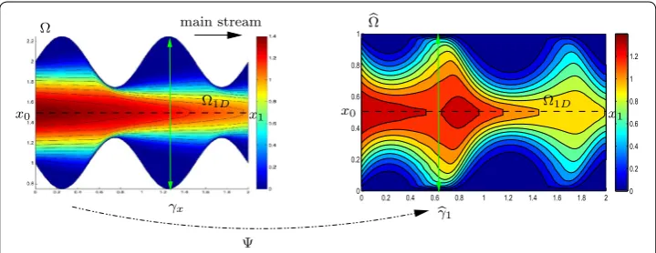
easier, free from undetermined constants, and are carried out once and for all. To this aim, for any x∈1D, we introduce the map ψx :γx →γd−1 between the generic fiber γx and the reference fiber γd−1⊂Rd−1. Maps ψx are instrumental to define the global map :→, where � =x∈�1D{x} ×γd−1 denotes the reference computational domain
(see Fig. 1 for an example of map ). Regularity assumptions are introduced on the maps
ψx and . In particular, we assume ψx to be a C1−diffeomorphism, for all x∈1D, and
to be differentiable with respect to z (essentially to exclude any kinks along Ŵ∗).
We also demand that the supporting fiber 1D is preserved by map , so that the generic point z=(x,y)∈� is mapped into z=�(z)=(x,y), with x≡x and
y=ψx(y) . Finally, without reducing the generality, we assume 1D to be the subset of
with y=0, i.e., 1D exactly coincides with the centerline of .
Remark 1 In a 2D setting, we may always select ψx as a linear transformation, so that
y=ψx(y)=y/L(x), with L(x)=meas(γx). In 3D a similar choice is possible only for
0 0.2 0.4 0.6 0.8 1 1.2 1.4 1.6 1.8 2 0
0.2 0.4 0.6 0.8 1
0 0.2 0.4 0.6 0.8 1 1.2
Ω
Ψ
γx
main stream
x0 x1 x1
Ω
x0
γ1
Ω1D Ω1D
specific configurations, for instance when is a cylindrical domain. In this case L(x)
coincides with the diameter of the pipe along the centerline.
HiMod reduction
The HiMod technique has been proposed in [9, 10] with the idea of exploiting the fiber structure demanded on , or, likewise, the preferential dynamics of the phenomenon at
hand. Currently, three versions of HiMod reduction have been investigated, from both a theoretical and a numerical viewpoint (see [13] for a survey on the different approaches). Independently of the selected technique, the idea is to manage in a different way the dependence of the solution on the leading and on the transverse dynamics. In particu-lar, since HiMod aims at providing enriched 1D models to be associated with the domi-nant direction, only the domidomi-nant dynamic is discretized via a standard finite element scheme, while getting information on the transverse dynamics via a modal expansion. In this section, we consider two of the available HiMod formulations.
Uniform HiMod reduction
The distinguishing feature of a uniform HiMod formulation is the adoption of a unique level of detail (i.e., the same number of modal functions) in modeling the transverse dynamics. For the sake of simplicity, we start from a steady setting. The function space associated with a uniform HiMod approach is
where m∈N+ is a given integer, V1D⊆H1
(�1D), and B= {ϕj}j∈N+ is a modal basis of functions in H1(γd−1), orthonormal with respect to the L2(γd−1)-scalar product. The
boundary conditions assigned on Ŵ0 and Ŵ1 are taken into account by the space V1D , while the boundary data on Ŵ∗ are included in B. Space Vm represents the hierarchy of models. We complete definition (3) by adding a conformity (Vm⊂V) and a spectral approximability (limm→+∞ infvm∈Vm�v−vm�V =0, for any v∈V) hypothesis on Vm [9, 10].
Remark 2 The analysis below is completely general with respect to the boundary data.
So far the robustness of the HiMod reduction has been verified when either homogene-ous Dirichlet or homogenehomogene-ous Neumann boundary conditions are assigned on Ŵ0, Ŵ1,
Ŵ∗, or when non-homogeneous Dirichlet data are enforced on Ŵ0 and Ŵ1. In general, the critical point is the identification of a basis B matching Robin boundary conditions or non homogeneous data on Ŵ∗. A new strategy with respect to this issue has been recently
proposed in [31].
With a view to unsteady problems, we introduce a time partition of the time win-dow I into N subintervals In=(tn−1,tn] of width kn=tn−tn−1, for n=1,. . .,N, with
k=maxnkn, t0≡0 and tN ≡T. This partition induces a subdivision of the cylinder Q into N space–time slabs Sn=×In, with n=1,. . .,N. Notice that partition {ti}Ni=0
(3)
Vm=
vm(x,y)= m �
j=1
�
is not necessarily uniform, to match the possible time heterogeneities of the problem. Now, we look for an approximate solution to (2) coinciding, on each space–time slab Sn, with a polynomial of degree at most q in time, with q∈N+, and with an element of Vm in
space, i.e., a function of the reduced space
The boundary conditions in (2) identifies V1D with Hγ1D(�1D), where γD is a subset of
{0, 1} according to the definition of ŴD, while functions ϕj,r belong to the modal basis B. Moreover, since 0�∈I1, the value vm(x,y, 0) has to be specified separately.
A priori, functions in VmN may exhibit a discontinuity at each time level, with continuity
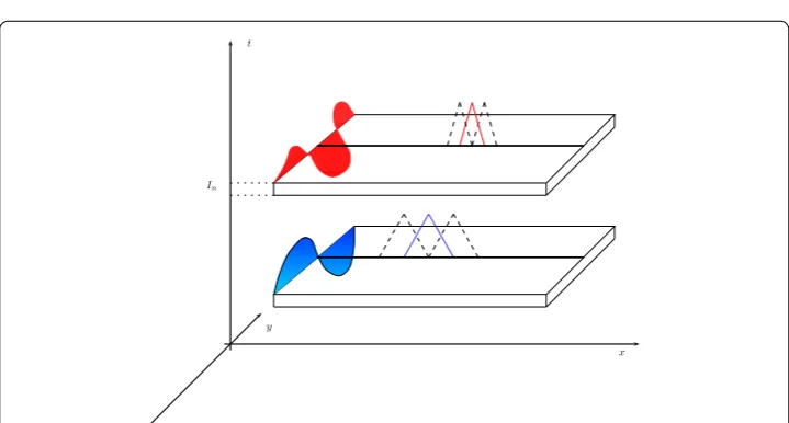
from the left. As a consequence, a different number of modal functions can be selected on each time interval In (see Fig. 2). This choice leads to replace in (4) the modal index m with the index mn∈N+ with n=1,. . .,N. In such a case we adopt the term space–time
slabwise uniform HiMod reduction and we change the notation in (4) into VmN, where
m= [m1,. . .,mN]′∈
N+N is the vector that collects the number of modes used on
each interval In, with vm the generic function in VmN.
The possible time discontinuity in VmN leads us to distinguish between the values vmn,+=limt→0+vm(x,y,tn+t) and vnm,−=limt→0+vm(x,y,tn−t), and to define the temporal jump [vm]n=vmn,+−vmn,− at the generic time tn, for n=0,. . .,N−1. Notice that this jump is identically equal to zero for functions in V. This remark allows us to provide a weak formulation for problem (1) equivalent to (2): find u∈V such that
(4)
VmN =
vm:(0,T] →H
1
ŴD(�): ∀n=1,. . .,N
vm(x,y,t)
� �
In =
q
�
r=0
m
�
j=1
tr�vjn,r(x) ϕj,r(ψx(y)), with �vjn,r ∈V1D
.
(5)
AcGdG(u,v)=FcGdG(v) ∀v∈V,
y
x t
In
where, for any w, ζ ∈V,
with u0,+=u0,−
=u0(x,y) and ∂QnN =ŴN×In for n=1,. . .,N. The space–time
slab-wise uniform HiMod formulation can thus be stated: find um∈VmN such that, for any
vm∈VmN,
The jump terms in (6) provide now an actual contribution, and we distinguish between the HiMod approximation u0,m−∈VmN|I1 of the initial datum u0 and u
0,+
m that is unknown. The conformity and the spectral approximability hypotheses are now added slabwise to guarantee the well-posedness of formulation (8). Indeed, due to the discontinuity in time, we can only expect that VmNS
n ⊂V
Sn, while V N m �⊂V.
Concerning the spatial discretization, following [9, 10], we consider a finite ele-ment discretization of the function dependence on x, after introducing a subdivi-sion, not necessarily uniform, of 1D into subintervals. The time discontinuity allows
to employ a different 1D mesh on each space–time slab (see Fig. 2). In particular, we denote by Thn = {Kln}Mn
l=1 the spatial partition associated with Sn for n=1,. . .,N, with Kln=(xln−1,xnl) the generic subinterval of width hnl =xln−xnl−1 for l=1,. . .,Mn ,
with hn=maxlhnl and xn0≡x0, xMn n ≡x1. Then, we furnish each Sn with the space Xh1D,s
n of the conforming finite elements of degree s associated with Thn, and with dim(Xh1D,s
n )=Nhn<+∞. A standard density hypothesis in V1D is advanced on each finite element space. Thus, the discrete counterpart of formulation (8) is: find uhm∈Vm,Nh such that, for any vhm∈Vm,Nh,
where
(6)
AcGdG(w,ζ )= N
�
n=1
�
Sn
∂w
∂tζd�dt+ �
In
a�w,ζ�dt
+ N−1
�
i=1
�
�[
w]iζi,+d�+
�
�
w0,+ζ0,+d�
(7) FcGdG(ζ )=
�
�
w0,−ζ0,+d�+
N
�
n=1
�
Sn
fζd�dt+ �
∂QnN
gζds dt
,
(8)
AcGdG(um,vm)=FcGdG(vm).
(9)
AcGdG(uhm,vmh)=FcGdG(vmh),
(10)
Vm,Nh=
v
h
m:(0,T] →H 1
ŴD(�): ∀n=1,. . .,N
vhm(x,y,t)
� �
In=
q
�
r=0
mn
�
j=1
tr�vjn,r,h(x) ϕj,r(ψx(y)), with �v n,h j,r ∈X
1D,s hn ∩V1D
uhm,0,−∈VmN,h|I1 is a discrete HiMod approximation of u0, and uhm,0,+ is an unknown.1 It follows Vm,Nh⊂VmN, i.e., also the discrete HiMod space Vm,Nh consists of functions
contin-uous in space but discontincontin-uous in time. Notice that, although Vm,Nh�⊂V, in (9) we can
extend definitions (6) and (7) to Vm,Nh taking advantage of the slabwise splitting.
By generalizing the notation used in [14–16] to denote finite elements that are con-tinuous in space and disconcon-tinuous in time, we refer to Vm,Nh as to the HiMod c[M(m)
G(s)]-dG(q) space (and, analogously, to (9) as to the c[M(m)G(s)]-dG(q) HiMod
formu-lation). We mean that, on each Sn, the full solution is replaced by a reduced solution continuous in space and discontinuous in time, obtained via a Galerkin approximation based on finite elements of degree s combined with the modal expansion associated with the multi-index m to discretize the space, and piecewise polynomials of degree q for the
time discretization.
The finite element discretization along 1D allows us to further expand the Fourier
coefficient vjn,r,h in (10) in terms of the finite element basis {ϑl} Nhn
l=1 associated with space
Xh1D,s
n , so that any function v
h
m∈Vm,Nh can be represented on the generic time interval In as
with n=1,. . .,N. The coefficients ujn,r,h,l of uh
m become the actual unknowns of the c[M(m )G(s)]-dG(q) HiMod formulation (9).
HiMod versus PGD
Following the classification proposed in [5], both HiMod reduction and PGD can be cat-egorized as a priori approaches since they do not rely on any solution to the problem at hand as, for instance, a POD strategy. Both the methods involve the weak form of the full problem and are based on a classical separation of variables. Nevertheless, while HiMod reduction applies this separation only to the space–time coordinates, PGD involves also problem parameters, such as boundary conditions or material properties, thus increas-ing the dimension of the space of the unknowns. HiMod applies a different discretization to the variables based on the physics of the problem. The accuracy for each variable may be tuned locally via a posteriori arguments. A PGD approach replaces in (3) the known modal function ϕj(ψx(y)), with y=(y,z)′, with a term of the form Fj(y)Gj(z) , with Fj and Gj unknowns. The two procedures both lead to 1D algebraic systems. In PGD they are intrinsically nonlinear and, in general, of large dimension. PGD requires therefore specific methods for the nonlinearity. In addition, the construction of the PGD approxi-mation via a successive enrichment of an initial solution closely resembles the heuristic approach initially used in HiMod for selecting the number of transverse modes [10]. In this respect, the automatic selection of the HiMod approximation in [11] may represent an important evolution in a PGD setting as well.
1 To simplify notations, with the super-index h we understand both the space and time discretizations.
(11)
vhm(x,y,t)In = q
r=0
mn
j=1
Nhn
l=1
Pointwise HiMod reduction
A fixed number of modal functions on the whole may be too restrictive in the presence
of spatial heterogeneities. This justifies the formalization of HiMod strategies alternative to the uniform approach, where a different number of modes is adopted in different sub-domains of (via a piecewise HiMod reduction [10, 11]), rather than in correspondence
with each finite element node (thanks to a pointwise HiMod formulation [12]). We focus on the last approach. The numerical verification in [12] identifies the pointwise method as the best-performing one in the presence of either widespread or localized transverse dynamics.
The idea exploited in a pointwise HiMod expansion consists in rewriting (11) by emphasizing the sum on the finite element nodes, as
and then in making the modal index mn dependent on the nodal index l. Space Vm,Nh is
thus replaced by the new space
where Mn= [mn,1,. . .,mn,Nhn]′∈
N+Nhn is the modal nodewise vector collecting
the number of modes used at each finite element node of the slab Sn for n=1,. . .,N, whereas M is just the subindex used to denote a pointwise HiMod approximation. The
nodewise tuning of the number of modes leads to an algebraic system sharing the same sparsity pattern as for the uniform case, but with a smaller dimension [12]. The formula-tion related to space VM,Nh coincides with a space–time pointwise HiMod reduction and
will be denoted by c[M(M)G(s)]-dG(q) form. It reads exactly as (9), simply by replacing
space VmN,h with VMN,h. Notice that, since definition (12) strictly depends on the finite
ele-ment discretization, there does not exist a weak counterpart of the pointwise HiMod formulation.
Uniform versus pointwise HiMod reduction: an example
We compare the uniform and the pointwise HiMod approaches on the steady test case 4 in [10], where the transport of oxygen in a wavy channel, representing a Bellhouse oxy-genator for extra-corporeal circulation [32], is modeled. This problem is characterized by a widespread dynamics, that is suited to be reduced via both the HiMod techniques.
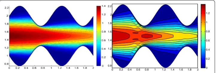
Figure 3, left shows the full solution u computed with FreeFem++ [33] on an unstructured uniform mesh of about 50,000 elements and via 2D affine finite elements. The irregular shape of the domain strongly affects the main stream of the flow on the whole domain as highlighted by the bent contour lines.
vmh(x,y,t) � �
In = Nhn �
l=1 ϑl(x)
q �
r=0 mn �
j=1
tr�vjn,r,h,lϕj,r(ψx(y)) ,
(12)
VMN,h=
v
h
M:(0,T] →H
1
ŴD(�): ∀n=1,. . .,N
vMh(x,y,t) � �
In=v
h
Mn(x,y,t)=
Nhn
�
l=1 ϑl(x)
q
�
r=0 mn,l �
j=1
tr�vjn,h,r,lϕj,r(ψx(y))
As far the HiMod reduction, we discretize the dependence of u on x via affine finite elements after introducing a partition of uniform step h=0.1 on 1D. The transverse
dynamics are described with a basis B of sinusoidal functions. To evaluate the integrals of the modal functions, we resort to Gaussian quadrature formulas based on four quad-rature nodes per wavelength, at least. No stabilization scheme is used. We first apply the uniform HiMod approach by resorting to 11 modal functions (see Fig. 3, right). Indeed, as shown in [10], at least 11 modes are required to obtain a sufficiently reliable HiMod approximation.
As second assessment, we build the pointwise HiMod approximation uhM associated
with the modal distribution M in Fig. 4, center. By comparing Fig. 3, right with Fig. 4,
left we recognize that the two reduced solutions are very similar. In particular, the inner-most contour lines associated with uhM are more accurate, despite the lower number of
dof involved by the pointwse approximation (48,400 dof characterize uh11 to be compared
with 28,282 dof for uhM, see the corresponding sparsity pattern in Fig. 4, right).
In accordance with [12], results in Figs. 3 and 4 show the improved modeling capabili-ties of the pointwise HiMod method vs the uniform approach, for a fixed computational effort. The main issue related to a pointwise formulation is the selection of the nodewise modal distribution. This corroborates the need for an automatic modal selection.
Adaptive HiMod reduction
Due to its significant impact on practical applications, we consider a goal-oriented framework (see, e.g., [17–19]), so that the predicted reduced model fits a goal func-tional representing a physical quantity of interest (e.g., mean or pointwise values, fluxes across sections or regions, the energy of the system, the vorticity of a turbulent flow). We denote by J the selected functional and we assume it is linear. We aim at approximating, within a prescribed tolerance TOL, the value J(u), with u solution to the full problem (2), via J(uhM), where uhM is the reduced solution identified by a preprocessing phase.
At this stage, we use a uniform and sufficiently fine discretization xnl,tn Mn
l=1 N
n=1 on
1D×I so that we can neglect the error due to the space–time discretization.
The a posteriori modeling error analysis
We generalize the error analysis in [11] to an unsteady setting, to automatically produce the HiMod lookup diagram that provides the number of modes to be switched on at
0 0.2 0.4 0.6 0.8 1 1.2 1.4 1.6 1.8 2 0.8
1 1.2 1.4 1.6 1.8 2 2.2
0 0.2 0.4 0.6 0.8 1 1.2
0
0.2
0.4
0.
6
0.
8
1
1.2
1.4
1.
6
1.
8
2
0.8
1
1.2
1.4
1.6
1.8
2
2.2
0
0.2
0.4
0.6
0.8
1
1.2
0
0.2
0.4
0.
6
0.
8
1
1.
2
1.
4
1.
6
1.
8
2
0
2
4
6
8
10
12
14
16
18
0
10
0
200
300
40
0
500
600
700
800
900
0
100 200 300 400 500 600 700 800 900
nz = 2828
2
Fig
. 4
W
av
y channel t
est case: node
wise H
iM
od solution (
left
) with cor
responding modal distr
ibution (
center
) and sparsit
y patt
er
n (
right
each finite element node and at each time of the space–time partition xnl,tn Mn
l=1 N
n=1 (see Fig. 7, left for an example). The a posteriori analysis is carried out on the slabwise uniform HiMod formulation, while the pointwise approximation uhM constitutes the
out-put of the adaptive procedure in the next section.
According to a goal-oriented approach, we introduce the dual problem associated with (8): find zm∈VmN such that, for any vm∈VmN,
where, for any ζ ∈V ∪VmN,
where j is the density function associated with the goal functional J. Notice that, since
VmN �⊂V, J has to be defined on V∪VmN and analogously for JcGdG. A null final condition,
zNm,+=0, allows to get rid of the first integral in (14), whereas boundary contributions may modify the definition of JcGdG when functional J involves a control on the boundary.
The assignment of boundary conditions to the dual problem is a crucial issue that is usu-ally tackled via the Lagrange identity.
Remark 3 The bilinear form AcGdG(w,ζ ) in (6) can be alternatively rewritten
integrat-ing by parts the time derivative and recombinintegrat-ing the jump terms as
for any w, ζ ∈V ∪VmN. This form better fits the dual setting due to the reverse time scale.
To derive the a posteriori modeling error estimator, we need to introduce the enriched primal and dual slabwise uniform HiMod problems,
with m+>m (i.e., m+
i >mi for i=1,. . .,N). The inclusion VmN ⊂Vm+N guarantees the orthogonality relations
The analysis derived in [11] can be applied to the slabwise uniform HiMod formulations, to state the following
Proposition 1 Let em=u−um∈V ∪VmN and em+ =u−um+∈V∪Vm+N be the
modeling error associated with the reduced formulation (8) and (15), respectively for
(13)
AcGdG(vm,zm)=JcGdG(vm),
(14) JcGdG(ζ )=
�
zmN,+ζN
,−
d�+
N
n=1
Sn
jζd�dt,
N
�
n=1
−
�
Sn ∂ζ
∂tw d�dt+ �
In
a�w,ζ�dt
−
N−1
�
i=1
�
�[
ζ]iwmi,−d�+
�
�
ζN,−wN,−d�,
(15)
find u+m∈Vm+N s.t. AcGdG(um+,vm+)=FcGdG(vm+) ∀vm+∈Vm+N ,
(16)
find z+m∈VmN+ s.t. AcGdG(vm+,zm+)=JcGdG(vm+) ∀vm+∈VmN+,
m,m+∈N+Nand withm+>m. Let us assume that the final dual datazN,+ m andzN
,+ m+
are identically equal to zero. Then, if there exists a positive constantσm<1and a modal
multi-indexM0∈N+Nsuch that, form+>m≥M0,
the following two-sided inequality holds
withδumm+ =um+−um.
Thanks to the requirement on the dual final data, we have that JcGdG≡J. Result (18)
identifies the estimator ηmm+ for the modeling error J(em) with the value |J(δumm+)| , while guaranteeing the efficiency and the reliability of ηmm+ via the lower and upper
bound, respectively. Following [11], to evaluate estimator ηmm+, we can adopt three
equivalent formulas, i.e.,
with δzmm+ =zm+−zm, and where ρp(um)(·)=FcGdG(·)−AcGdG(um,·), and
ρd(zm)(·)=JcGdG(·)−AcGdG(·,zm) denote the weak primal and dual residual
associ-ated with formulation (8) and (13), respectively. Moreover, to make computable ηmm+,
we replace the reduced primal and dual solutions with corresponding discrete approxi-mations. Estimator ηmm+ exhibits the structure typical of a hierarchical error estimator,
yet in a goal-oriented framework. We refer to [11] for further computational remarks and for some considerations on hypothesis (17) that represents a generalization of the standard saturation assumption [34–36] to a goal-oriented setting.
Construction of the HiMod lookup diagram
Estimator ηmm+ is now used to automatically select the pointwise HiMod approximation uhM for problem (2) that guarantees the desired accuracy TOL on the functional error
J(u−uhM).
To start the adaptive algorithm, we assign two initial (possibly small) values to the uni-form modal indices m and m+. Then, we resort to the following five-stage procedure:
(S1) we compute the discrete uniform reduced primal and dual solutions, uhm, uhm+, zm, zhm+, on the whole space–time cylinder Q;
(S2) we evaluate the modeling estimator ηnmm+ =ηmm+
Sn localized to each space–
time slab Sn;
(S3) we apply the adaptive procedure outlined in Fig. 5 on each slab Sn to predict the
corresponding nodewise modal distribution Mn, i.e., to build the HiMod lookup
diagram (see below for all the details);
(S4) we compute the discrete pointwise reduced primal and dual solutions, uhM, uhM+,
zM, zMh+, associated with the HiMod diagram yielded at stage (S3);
(S5) we evaluate the global modeling error estimator ηMM+ by employing the point-wise solutions identified at stage (S4). Then, if the global tolerance is met, i.e.,
(17)
|J(em+)| ≤σm|J(em)|,
(18)
|J(δumm+)|
1+σm ≤ |J(em)| ≤
|J(δumm+)| 1−σm ,
(19)
ηMM+ ≤ TOL, the procedure stops, providing the HiMod lookup diagram in (S3)
as final outcome. Vice versa, if ηMM+>TOL, we come back to (S2).
Before detailing the adaptive procedure at stage (S3), some remarks are in order.
The computational effort associated with stage (S1) takes advantage of the time dis-continuity of the c[M(M)G(s)]-dG(q) scheme. More sophisticated approaches such as
checkpointing [37] may be adopted to further reduce the computational costs. The mod-eling estimator can obviously be evaluated in correspondence with any HiMod approxi-mation [uniform as in (S2), slabwise uniform as in (19), pointwise as in (S5)]. Indeed, via the first definition in (19), it suffices to properly evaluate the bilinear form (6). Concern-ing the localization of the estimator to Sn at stage (S2), by exploiting again the first defi-nition in (19), we have
Finally, the HiMod pointwise approximations uhM, zhM and uhM+, zhM+ at stage (S4) are the
solutions to problems (5), (13) and (15), (16) settled in the space VM,Nh and VMN+,h,
respec-tively. In particular, we assume that VM,Nh and VMN+,h share the same spatial partitions Thn for n=1,. . .,N, so that M+ identifies reduced solutions with a pointwise larger number
of modes with respect to uhM and zMh.
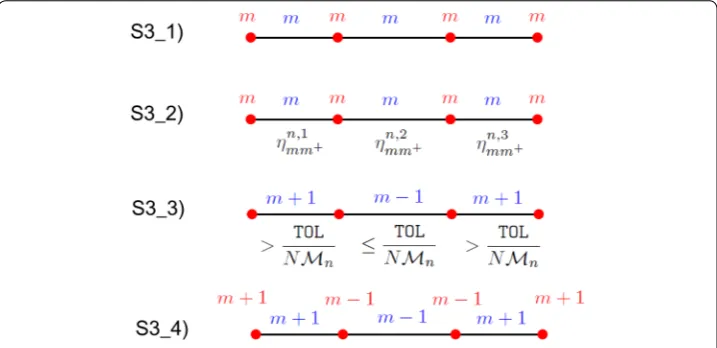
Let us focus now on the adaptive procedure devised to commute the slabwise evalua-tions of ηmm+ into the lookup diagram predicted at stage (S3). We focus on the generic
space–time slab Sn and on the case of linear finite elements:
(S3_1) we assign a number of modes equal to m to each node and to each subinterval of partition Thn;
(20)
ηmmn +=AcGdG(δumm+,δzmm+)
Sn
=
Sn
∂δumm+
∂t δzmm+d�dt+
In
aδumm+,δzmm+dt+
�
(S3_2) we evaluate the estimator ηnmm,l + =ηnmm+Kn
l localized to each interval K
n l of Thn,
for l=1,. . .,Mn;
(S3_3) we invoke an equidistribution criterion on the slabs as well as on the subinter-vals Kln. If ηnmm,l + >TOLδ1M/(NMn), we increase by one the modal index
associ-ated with Kln (model refinement); if ηmmn,l +<TOL δ2M/(NMn), we decrease by
one such an index (model coarsening); otherwise, we preserve the current modal index;
(S3_4) we update the number of modes associated with each finite element node by assigning to the generic node xnl, for l=1,. . .,Mn−1, a number of modes
equal to mn,l=min(mKln,mKln+1), with mK n
l the number of modes assigned
on the interval Kln . In particular, to avoid an abrupt variation of modes on
consecutive nodes, the actual value m∗n,l associated with xnl coincides with max(0.5mn,l−1+0.5mn,l+1−3,mn,l) . The endpoints of 1D are updated
sepa-rately as mn,0=mKn
1 and mn,Mn=mKMn n if Dirichlet boundary conditions are
not imposed on Ŵ0 and on Ŵ1, respectively. The assignment of the modal indices mn,l predicts the modal multi-index Mn= [mn,1,. . .,mn,Nhn]′ for the slab Sn.
The procedure in (S3) is exemplified in Fig. 5 for a partition Thn of 1D consisting only of
three subintervals Kln (l=1, 2, 3).
Of course, steps (S3_1)–(S3_4) are replayed on the enriched modal index m+, with a view to the evaluation of the modeling error estimator at stage (S5).
The adaptive modal algorithm includes both model refinement and coarsening. A min-imum number of modes constrains the modal coarsening, while a maxmin-imum number of adaptive iterations is fixed to avoid too restrictive demands on TOL. The tuning parame-ters δ1M and δ2M at stage (S3_3) make the adaptive algorithm more robust, while
increas-ing the correspondincreas-ing computational efficiency. We set δ1M=0.5, δ2M=1.5. Finally, the
modal update at step (S3_4) plays a crucial role since it explains how to build a pointwise HiMod approximation uhM starting from a HiMod lookup diagram, where the modes are
associated with the subintervals.
Numerical verification
The numerical verification is carried out in a 2D setting. Moreover, to select the discrete HiMod space, we choose q =0 and s=1, i.e., we use linear finite elements to discretize
the leading dynamics and functions piecewise constant in time. It can be checked that the adopted time discretization is equivalent to a modified backward Euler scheme [15].
Reliability of the adaptive HiMod reduction procedure
We approximate problem (1) on the rectangular domain �=(0, 3)×(0, 1) for t∈I=(0, 1), and by choosing Lu= −u+c· ∇u, with c= [10, 0]′. Besides the
u approximated with FreeFem++ via a standard 2D cG(1)-dG(0) scheme on a uni-form unstructured mesh of 10252 triangles. As expected, the convective field acts on the purely diffusive phenomenon by horizontally bending the contour lines. From a mod-eling viewpoint, we are simulating, for instance, the process of convection and diffusion of a pollutant emitted by a chimney localized at D, in the presence of a moderate
hori-zontal wind. In this context, the full solution u(t) represents the pollutant concentration in the domain at a certain time t∈I
We aim at controlling the mean value of the full solution on the whole at the final time T =1, i.e., we select the goal functional J as Jmean,T(ζ )= [meas(�)]−1
�ζ (x,y, 1)d�. The choice of a localized functional is challenging with a view to the mod-eling adaptive procedure. The dual problem is characterized by the differen-tial operator L∗z= −z−c· ∇z, with source term given by the density function j(x,y,t)= [meas(�)]−1δT associated with Jmean,T, where δT denotes the Dirac
distribu-tion associated with the final time. On ŴN a homogeneous Robin boundary condition is
imposed, while a homogeneous Dirichlet data is assigned on ∂�\ŴN. A null final value
zN,+
m is selected.
Both the primal and dual problems are computed by discretizing the supporting fiber
(0, 3)× {0.5} via a uniform partition of size h=0.15 and the time window with a con-stant step k=0.1. The modal basis B consists of sinusoidal functions.
Finally, the modeling tolerance TOL is set to 10−2
, while the uniform modal indices m
and m+ are set to 1 and 3, respectively.
0 0.5 1 1.5 2 2.5 3
0 0.2 0.4 0.6 0.8 1 0 0.02 0.04 0.06 0.08 0.1 0.12
0 0.5 1 1.5 2 2.5 3
0 0.2 0.4 0.6 0.8 1 0 0.02 0.04 0.06 0.08 0.1 0.12
0 0.5 1 1.5 2 2.5 3
0 0.2 0.4 0.6 0.8 1 0 0.02 0.04 0.06 0.08 0.1 0.12
0 0.5 1 1.5 2 2.5 3
0 0.2 0.4 0.6 0.8 1 0 0.02 0.04 0.06 0.08 0.1 0.12
0 0.5 1 1.5 2 2.5 3
0 0.2 0.4 0.6 0.8 1 0 0.02 0.04 0.06 0.08 0.1 0.12
0 0.5 1 1.5 2 2.5 3
0 0.2 0.4 0.6 0.8 1 0 0.02 0.04 0.06 0.08 0.1 0.12
0 0.5 1 1.5 2 2.5 3
0 0.2 0.4 0.6 0.8 1 0 0.02 0.04 0.06 0.08 0.1 0.12
0 0.5 1 1.5 2 2.5 3
0 0.2 0.4 0.6 0.8 1 0 0.02 0.04 0.06 0.08 0.1 0.12
0 0.5 1 1.5 2 2.5 3
0 0.2 0.4 0.6 0.8 1 0 0.02 0.04 0.06 0.08 0.1 0.12
0 0.5 1 1.5 2 2.5 3
0 0.2 0.4 0.6 0.8 1 0 0.02 0.04 0.06 0.08 0.1 0.12
Fig. 6 Convection–diffusion of a pollutant, control of Jmean,T, modal adaptation: full solution (left) and HiMod
approximation uh
0
0.5
1
1.5
2
2.5
3
0
1
2
3
4
5
6
7
8
9
10
0
1
2
3
4
5
6
7
x 10
−4
0
0.5
1
1.5
2
2.5
3
0
1
2
3
4
5
6
7
8
9
10
2
4
6
8
10
12
0
0.1
0.2
0.
3
0.4
0.
5
0.
6
0.7
0.
8
0.
9
0
2
4
6
8
10
12
14
Fig
. 7
C
on
vec
tion–
diffusion of a pollutant, contr
ol of
Jmean
,
T
, modal adaptation: H
iM
od look
up diag
ram (
left
); modal distr
ibution at x
= 1.5 as a func
tion of time (
center
); space
–time distr
ibution of
ηM
M
+
(
right
The adaptive algorithm converges after 21 iterations and provides as output the HiMod lookup diagram in Fig. 7, left. The diagram coincides with the space–time rectangle
1D×I, where 1D and I exhibit the corresponding partition of uniform size h and k,
respectively. A certain number of modal functions is associated with each cell Kln×k for l=1,. . .,Mn and n=1,. . .,N. Thus, by resorting to the procedure in Fig. 5, (S3_4) it is possible to build the HiMod pointwise approximation uhM
n for n=1,. . .,N, i.e., the reduced solution uhM that guarantees the estimate |Jmean,T(u)−Jmean,T(uhM)|<TOL.
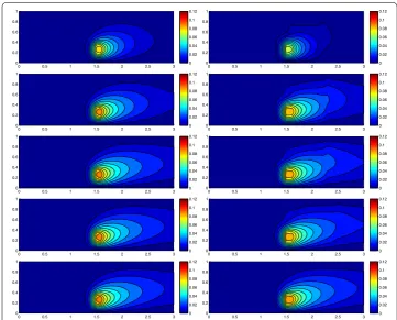
The HiMod diagram in Fig. 7, left shows that few modes are demanded on the whole space–time domain, except for the two last time intervals, where a larger number of modes is switched on in correspondence with the localized source and the downstream region. More quantitative information are provided by the plot in Fig. 7, center of the number of modes associated with node x=1.5 as a function of time. Only three modes are used on the whole time interval except for the subintervals IN−1 and IN, when five
and 13 sine functions are required, respectively. The modal distribution predicted by the lookup diagram is completely coherent with a goal-oriented approach. Since we are interested in the mean value of the solution only at the final time, it is reasonable to expect a reliable approximation of the full solution only in correspondence with the last time intervals. This trend is confirmed by the corresponding pointwise HiMod approxi-mation which reproduces more closely the full one during the last times of the simula-tion (compare Fig. 6, left and right).
In Fig. 7, right we show the value of ηMM+ on the same space–time structure of the
HiMod diagram. The boxes associated with the largest values of the estimator identify a pattern similar to the one in Fig. 7, left.
Sensitivity of the adaptive HiMod reduction procedure to the goal‑functional
We re-run the adaptive procedure by preserving all the input parameters, but for J =Jmean,left T(ζ )= [meas(�
left
)]−1�leftζ (x,y, 1)d�left, with �left=(0, 1.2)×(0, 1). We deal now with a functional localized both in time and space. The adaptive procedure stops after only three iterations by providing the HiMod lookup diagram in Fig. 8, left. A single mode is adopted on the whole time interval in left where the solution is flat. To
ensure tolerance TOL, the modeling error estimator identifies the portion of the domain around D as the most problematic one. As a consequence, three sinusoidal functions are
0 0.5 1 1.5 2 2.5 3
0 1 2 3 4 5 6 7 8 9 10
1 1.2 1.4 1.6 1.8 2 2.2 2.4 2.6 2.8 3
0 0.5 1 1.5 2 2.5 3 0
0.2 0.4 0.6 0.8 1
0 0.02 0.04 0.06 0.08 0.1 0.12
Fig. 8 Convection–diffusion of a pollutant, control of Jmean,T, modal adaptation: HiMod lookup diagram (left); left HiMod approximation uh
used in the two consecutive spatial intervals just before x=1.5 for the whole temporal window, except for the last time interval, when a single mode is employed on the entire
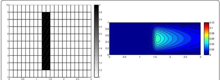
. The c[M(M)G(1)]-dG(0) HiMod approximation at the final time is shown in Fig. 8,
right. In agreement with a goal-oriented approach, the reduced solution is far from the full one at T in Fig. 6, left-bottom. The mean value is controlled in an area where the full solution is extremely smooth so that a single mode is enough.
Robustness of the HiMod lookup diagram
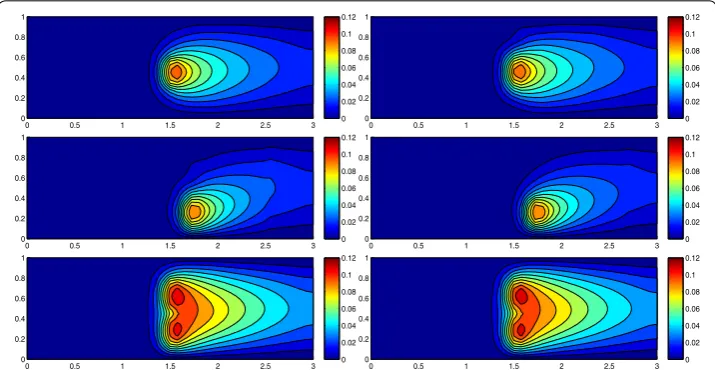
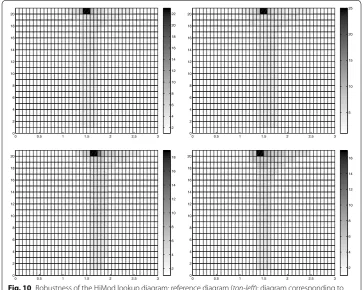
The computational effort demanded by the adaptive procedure is justified by the pos-sibility to employ the lookup diagram associated with a specific setting to hierarchi-cally reduce a variant of this. Figure 9 performs this check on three variants of the test-case in Fig. 6. In more detail, we adopt the HiMod lookup diagram in Fig. 10, top-left to build the HiMod approximation for three new advection-diffusion prob-lems, characterized by a different choice of the source term, namely, f1≡10χD1 with D1= {(x,y):(x−1.5)2+4(y−0.45)2≤0.01} (Fig. 9, top), f2≡10χD2 with
D2= {(x,y):(x−1.7)2+4(y−0.25)2≤0.01} (Fig. 9, middle) and f3≡10χD3 with
D3= {(x,y):(x−1.5)2+4(y−0.25)2≤0.01} ∪ {(x,y):(x−1.5)2+4(y−0.65)2≤0.01} (Fig. 9, bottom), respectively. Figure 9, left shows the HiMod approximations thus obtained. To check the reliability of the obtained solutions, we apply the HiMod adaptive algorithm directly to the three new problems. The corresponding lookup diagrams are gathered in Fig. 10, whereas the associated HiMod approximations are collected in Fig. 9, right. The matching between the contour plots in the two columns of Fig. 9 is substantial, in particular for the two-source test case which represents the most sigificant variant with respect to reference configuration.
As last investigation, we check the robustness of the HiMod lookup diagram with respect to the shape of the computational domain. This is a challenging issue due to the crucial role played by the maps ψx and in the HiMod reduction. For this reason,
0 0.5 1 1.5 2 2.5 3
0 0.2 0.4 0.6 0.8 1
0 0.02 0.04 0.06 0.08 0.1 0.12
0 0.5 1 1.5 2 2.5 3
0 0.2 0.4 0.6 0.8 1
0 0.02 0.04 0.06 0.08 0.1 0.12
0 0.5 1 1.5 2 2.5 3
0 0.2 0.4 0.6 0.8 1
0 0.02 0.04 0.06 0.08 0.1 0.12
0 0.5 1 1.5 2 2.5 3
0 0.2 0.4 0.6 0.8 1
0 0.02 0.04 0.06 0.08 0.1 0.12
0 0.5 1 1.5 2 2.5 3
0 0.2 0.4 0.6 0.8 1
0 0.02 0.04 0.06 0.08 0.1 0.12
0 0.5 1 1.5 2 2.5 3
0 0.2 0.4 0.6 0.8 1
0 0.02 0.04 0.06 0.08 0.1 0.12
we focus on a steady setting, in particular on the one in Fig. 3. We consider two vari-ants of the wavy-shaped domain. With the first one, we simply reduce the height of the sinusoidal sections (see Fig. 11, top), whereas in the second variant we add a rectangu-lar channel at the beginning and at the end of the original geometry (see Fig. 11, bot-tom). Figure 11 compares the solution computed on the modal distribution in Fig. 4, center with the HiMod approximation provided by the adaptive HiMod procedure. As
0 0.5 1 1.5 2 2.5 3
0 2 4 6 8 10 12 14 16 18 20 2 4 6 8 10 12 14 16 18 20 22
0 0.5 1 1.5 2 2.5 3
0 2 4 6 8 10 12 14 16 18 20 2 4 6 8 10 12 14 16 18
0 0.5 1 1.5 2 2.5 3
0 2 4 6 8 10 12 14 16 18 20 2 4 6 8 10 12 14 16
0 0.5 1 1.5 2 2.5 3
0 2 4 6 8 10 12 14 16 18 20 5 10 15 20 25
Fig. 10 Robustness of the HiMod lookup diagram: reference diagram (top-left); diagram corresponding to the source term f1 (top-right), f2 (bottom-left) and f3 (bottom-right)
0 0.2 0.4 0.6 0.8 1 1.2 1.4 1.6 1.8 2 1 1.2 1.4 1.6 1.8 2 0 0.2 0.4 0.6 0.8 1 1.2 1.4
0 0.2 0.4 0.6 0.8 1 1.2 1.4 1.6 1.8 2 1 1.2 1.4 1.6 1.8 2 0 0.2 0.4 0.6 0.8 1 1.2 1.4
−1 −0.5 0 0.5 1 1.5 2 2.5 3 0.8 1 1.2 1.4 1.6 1.8 2 2.2 0 0.2 0.4 0.6 0.8 1 1.2
−1 −0.5 0 0.5 1 1.5 2 2.5 3 0.8 1 1.2 1.4 1.6 1.8 2 2.2 0 0.2 0.4 0.6 0.8 1 1.2
expected, the matching between the two approximations is very good in Fig. 11, top. Despite the abrupt change in the domain shape, we get acceptable results also for the second geometric variant, thus confirming the good robustness of the HiMod lookup diagram with respect to possible changes of the original problem.
Combined HiMod reduction and space–time adaptation
Goal of this section is to enrich the information provided by the HiMod lookup diagram by predicting also the space–time partition of 1D×I. Consequently, we remove any
assumption on the finite element discretization as well as on the time partition {In}. In practice, we expect to replace the diagram in Fig. 7, left with a new diagram character-ized by a non uniform horizontal (spatial) and vertical (temporal) spacing.
The a posteriori estimator for the global error
With a view to a global adaptation, following, e.g., [11, 20–22], we derive an a posteriori
estimator for the global error Emh =em+ehm, where the contributions of the modeling (em=u−um) and of the discretization (emh =um−uhm) errors remain distinct. In par-ticular, since we are interested also in an adaptive selection of the space and time step size, we expect that the estimator for the discretization error consists of a spatial contri-bution separate from the temporal one [23–26].
As for the adaptive HiMod reduction, we carry out the a posteriori analysis in a slab-wise uniform HiMod setting. The following statement plays a crucial role in the defini-tion of the global error estimator.
Proposition 2 We assume that saturation assumption (17) holds, and we choose
zNm,+=zmN,++=0. Then, for anym, m+∈
N+N, withm+>m≥M0 and M0defined as
in Proposition1, it turns out that
Moreover, if there exists a constantwith0<<1, such that
it additionally holds that
Proof Estimates (21) and (23) follow from Propositions 3 and 4 in [11], respectively.
Starting from Proposition 2, we adopt the quantity
as a posteriori error estimator for the global error Eh
m. As a consequence, inequalities (21) and (23) state the reliability and the efficiency of such an estimator. The first term of ηmmh + exactly coincides with the modeling error estimator in (19), while the second
(21)
|J(Emh)| ≤ 1
1−σm
(|J(δumm+)| + |J(ehm)|).
(22)
|J(ehm)| ≤|J(em)|,
(23)
|J(Emh)| ≥ 1−
3+σm−
(|J(δumm+)| + |J(emh)|).
(24)
contribution takes into account the error associated with both the spatial and the tem-poral discretizations. The main effort of this section will be to explicitly estimate this term, with the additional requirement of distinguishing the space from the time contri-bution. As in [11], we modify the standard goal-oriented analysis to tackle the intrinsic dimensionally hybrid nature of a HiMod reduced formulation.
Concerning hypothesis (22), it essentially coincides with a sufficient grid resolution requirement since establishing a ratio between the modeling and the discretization errors. With a view to estimate |J(ehm)|, we preliminarily prove the following Galerkin orthogonality property for the discretization error ehm.
Lemma 1 For anyvhm∈Vm,Nh, the following relation holds
Proof We consider the HiMod formulation (8) and the corresponding discrete
coun-terpart (9). The time discontinuity characterizing spaces VmN and Vm,Nh allows us to select
the values of vm and vmh independently on each In for n=1,. . .,N. Thus, we pick both vm and vmh to vanish outside In so that formulations (8) and (9) reduce to a unique equation on In: find um∈VmN
Sn such that, for any vm∈V N
m
Sn,
and, likewise, find uhm∈VmN,h
Sn such that, for any v h m∈VmN,h
Sn,
with AcGdG(w,ζ )Sn defined as in (20) and
with w, ζ ∈V∪Vmh. Now, since VmN,h
Sn⊂V
N
m
Sn, we subtract (27) from (26) after identi-fying vm with vhm, to get the orthogonality relation
for any n=1,. . .,N. Identity (28) can now be generalized to an arbitrary function
vmh ∈Vm,Nh by suitably summing through the slabs. This yields identity (25).
Some notations are now instrumental. Let Rnl be the region of defined by
x∈Kn
l {x} ×γx, with K
n
l the generic subinterval of Thn, while we denote the interface between Rnτ and Rnτ+1 by ζτn, for τ =1,. . .,Mn−1 and n=1,. . .,N, and with ζ0n≡Ŵ0 and ζMn n ≡Ŵ1. Finally, SRn
l =R
n
l ×In denotes the space–time prism associated with Rnl,
(25)
N �
n=1 �
Sn
∂eh
m ∂t v
h
md�dt+
�
In
a�ehm,vhm
�
dt+
�
�[
ehm]n−1vhm,n−1,+d�
=
0.
(26)
AcGdG(um,vm)
Sn=FcGdG(vm)
Sn,
(27)
AcGdG(uhm,vmh)
Sn=FcGdG(v h m)
Sn,
FcGdG(ζ )
Sn=
Sn
fζd�dt+
∂QnN
gζds dt,
(28)
AcGdG(ehm,vmh)
while LRn l =∂R
n
l ×In identifies the corresponding lateral surface. We introduce now the spatial and temporal local residuals. For a fixed time interval In and for any Rnl, we con-sider the internal residual
and the boundary residual
associated with the discrete HiMod solution uhm, with l=1,. . .,Mn and n=1,. . .,N , where Lnl is the restriction of the elliptic operator L in (1) to the prism SRnl and [∂νuhm] is the jump of the conormal derivative of uhm across an edge of the skeleton Ehn= {ζτn}
Mn−1
τ=1 .
We consider now the temporal residual associated with uhm and with the time level tn
together with the initial error
Finally, we introduce the time projection operator Tn:VmN
Sn →H
1
ŴD(�), for
n=1,. . .,N, such that
and the one-dimensional Clément quasi-interpolant I1
:L2(�1D)→R [38]. By defini-tion, the projection error v−Tnv is orthogonal to any function c constant in time, so
that
whereas the estimate
can be proved [16]. Notice that no constant is involved in this result. Concerning the Clément quasi-interpolant, the estimates
(29)
rRn l =
f − ∂u
h
m ∂t −L
n luhm
SRn l
jRn
l =
0 on(∂Rnl ∩ŴD)×In
2(g−∂νuhm)|SRn l
on(∂Rnl ∩ŴN)×In
−[∂νuhm] on(∂Rln∩Ehn)×In
(30) Jn= [−uhm]n=(−umh,n,++uhm,n,−),
(31)
ehm,0,−=u
0,−
m −uh
,0,−
m .
Tnv=
1
kn
In
v dt ∀v∈VmNS
n,
(32)
In
(v−Tnv)c dt=0 ∀v∈VmN
Sn,
(33)
�v−Tnv�L2(In)≤kn
∂v
∂t
L2(In) ∀v∈V
N
m
Sn
(34)
�v−I1(v)�L2(K)≤C1hK|v|
H1(K)
(35)
�v−I1(v)�L2(∂K)≤C2h 1/2
hold, for any v∈H1(�1D), where K denotes a generic interval of 1D, K is the associated
patch of elements, and with C1 and C2 constants depending on the relative size of the
ele-ments constituting K [38].
We are now ready to prove the following result:
Proposition 3 Let⊂R2. Let us assume that the approximationuhm,0,−of the initial
datum coincide with theL2-projectionPI1(um0,−)ofu0,m−onto the spaceVm,Nh
I1. Moreover,
we choosezmN,+=0. Then, the following estimate for the functional error|J(ehm)|holds
withCa constant depending on the interpolation constants in (34) and (35), onqand on
maxnmn, where the residuals are defined by
withrRn
l =TnrRnl, jRnl =TnjR n l, h
n
l andknthe length of the generic subintervalKlnandIn,
respectively forl=1,. . .,Mnandn=1,. . .,N, and withδ1,nthe Kronecker symbol
asso-ciated with the first slabS1, while the weights are given by
with
the patch associated with the subinterval Kln, L(x)=meas(γx), zjn,r andz
n,h
j,r the modal
coefficients associated with the dual solutionzmand with the corresponding
discretiza-tionzmh, respectively.
Proof We start from the dual problem (13) by choosing vm=ehm and we apply the
orthogonality relation (25). It follows that, for any vh
m∈Vm,Nh,
(36)
|J(ehm)| ≤C N
n=1
Mn
l=1
ρRSn
l(u
h
m) ωSRnl(zm−zmh)+ 2
i=1
ρRTin l(u
h
m) ωTiRnl(zm−zhm)
,
ρRSn l(u
h
m)=hnl�rRn l�L2(SRn
l)+ 1 2(h
n l)
1 2�j
Rnl�L2(LRn l) , + h n l k 1 2 n
(�Jn−1�L2(Rn l)+ �e
h,0,−
m �L2(Rn l)δ1,n),
ρT1
Rn l(u
h
m)=kn�rRnl −rRln�L2(S
Rn l)+
k
1 2
n(�Jn−1�L2(Rn l)+ �e
h,0,−
m �L2(Rn l)δ1,n),
ρT2
Rn l(u
h m)=
kn
2 �jRnl −jRnl�L
2(L
Rnl),
ωSRn l(zm−z
h m)=
max
x∈Kn l
L(x)
1
2q
r=0
mn
j=1
�zjn,r−zn
,h
j,r �H1(Kn l)�t
r
�L2(I n)
ωT1
Rln(zm−z
h m)=
∂(zm−zmh)
∂t
L2(S Rn
l) , ωT2
Rnl(zm−z
h m)=
∂(zm−zmh)
∂t
L2(L Rn
l) ,
(37) �
Kln=
K1n∪K2n, for l=1,
Kln −1∪K
n l ∪K
n
l+1 for l=2,. . .,Mn−1
KMn
n−1∪K n
The identification of JcGdG(ehm) with J(ehm) follows from the requirement on the dual final datum. We add and subtract the value eh
,0,−
m
zm−vhm
0,+
d, by exploiting in (31) the
choice uh,0,−
m =PI1(u
0,−
m ) for the primal initial datum. A manipulation of the jump con-tributions combined with the definition of projection operator yields
After exploiting relation (26) with vm=zm−vmh, we integrate by parts on the regions Rnl:
Thanks to definitions (29) and (30), we have
We consider separately the four terms (I)–(IV). In particular, we choose vhm coinciding
with zhm+Tn(I1(zm−zmh)), with zhm the discrete HiMod approximation of the dual
J(ehm)=AcGdG(ehm,zm)
= N n=1 Sn
∂ehm ∂t (zm−v
h
m)d�dt+
In
a(ehm,zm−vhm)dt
−
�[
em]h n−1vmh,n−1,+d�
+
N−1
i=1
�[
ehm]izim,+d�+
�
emh,0,+zm0,+d�
. J(ehm)
= N
n=1
Sn ∂ehm
∂t (zm−v
h
m)d�dt+
In
a(emh,zm−vmh)dt
+
�[
ehm]n−1(zm−vhm)n−
1,+ d� + �
emh,0,−
zm−vhm
0,+ d� .
J(ehm)= N n=1 Mn
l=1
In
Rnl
f − ∂u
h
m
∂t −L n luhm
(zm−vhm)dRnl
+
∂Rnl∩ŴN
g(zm−vhm)ds−
∂Rnl
∂νuhm(zm−vmh)ds
dt
+
Rnl
[−uhm]n−
1
(zm−vmh)n−
1,+
dRnl
+
M1
l=1
R1
l
ehm,0,−
zm−vhm
0,+ dR1
l . (38) �
�J(ehm)
� �≤
N �
n=1
Mn
�
l=1
� � � � � � � SRn l
rRnl(zm−vhm)dRnldt � � � � � � � �� �
(I)
+ 12
� � � � � � � LRn l
jRn l(zm−v
h
m)dsdt
� � � � � � � �� �
(II)
+ � � � � � � Rn l
Jn−1(zm−vhm)n− 1,+
dRnl
� � � � � � �� �
(III)
+ M1 �
�l=1
� � � � � � R1 �l
ehm,0,−
�
zm−vhm
�0,+
dR�1
l � � � � � � �� �
(IV)