R E S E A R C H
Open Access
ASSERT: attack synthesis and separation
with entropy redistribution towards
predictive cyber defense
Ahmet Okutan
*and Shanchieh Jay Yang
Abstract
The sophistication of cyberattacks penetrating into enterprise networks has called for predictive defense beyond intrusion detection, where different attack strategies can be analyzed and used to anticipate next malicious actions, especially the unusual ones. Unfortunately, traditional predictive analytics or machine learning techniques that require training data of known attack strategies are not practical, given the scarcity of representative data and the evolving nature of cyberattacks. This paper describes the design and evaluation of a novel automated system, ASSERT, which continuously synthesizes and separates cyberattack behavior models to enable better prediction of future actions. It takes streaming malicious event evidences as inputs, abstracts them to edge-based behavior aggregates, and associates the edges to attack models, where each represents a unique and collective attack behavior. It follows a dynamic Bayesian-based model generation approach to determine when a new attack behavior is present, and creates new attack models by maximizing a cluster validity index. ASSERT generates empirical attack models by separating evidences and use the generated models to predict unseen future incidents. It continuously evaluates the quality of the model separation and triggers a re-clustering process when needed. Through the use of 2017 National Collegiate Penetration Testing Competition data, this work demonstrates the effectiveness of ASSERT in terms of the quality of the generated empirical models and the predictability of future actions using the models.
Keywords: Cyber security, Dynamic bayesian classifier, Clustering KL divergence
Introduction
As new system vulnerabilities are discovered and attack tools become even more prevalent, cyber attackers may employ a variety of evolving strategies with a plethora of exploits. Symantec’s 2017 Internet Security Threat Report (Symantec2017) suggested that attacking tactics contin-ued to change and many attackers used whatever tools on hand rather than focused on sophisticated techniques. This means how attackers penetrate into a network may be situational and diverse, depending on what they dis-cover and what is available. The diverse and changing tactics pose challenges for security analysts to recog-nize and comprehend the ongoing malicious activities and emerging threats. Imagine a system that can pro-cess a significant volume of observables produced by intrusion detection systems, and continuously synthesize
*Correspondence:[email protected]
Computer Engineering, Rochester Institute of Technology, Rochester, NY, USA
and update a manageable set of‘empirical attack models’ that reflect the different ‘how’, ‘where’, and ‘what’ attack activities are present in the network. Such a system will assist security analysts to prioritize and anticipate critical attacks, hence offering a robust predictive cyber defense even in the presence of evolving and diverse cyberattack tactics.
Traditional intrusion detection systems (Zhang et al. 2008; Li et al. 2012) differentiate malicious events from benign ones to alert security analysts for potentially mali-cious activities. It is not uncommon for analysts to be overwhelmed by the potentially significant volumes of false positives or less critical alerts due to scanning activ-ities. Alert correlation systems (Valeur et al.2004; Ning et al.2004; Yang et al.2009) attempt to match the intru-sion alerts with a priori known models based on expert knowledge from previously observed incidents. An attack episode, however, may be composed of multiple stages where the scanning techniques, exploits, and targets are
likely to change depending on the attackers’ knowledge, preference, or just situational. The notion of training with ground truth or sole reliance on expert knowledge will not be sufficient to provide timely and robust attack models that can be used to predict future attacks. Complementing existing intrusion detection and alert correlation works, this paper aims at separating intrusion alerts to generate emerging attack behavior models, some more critical than others, for better analyses and predictability. This paper presents ASSERT – a novel, automated and configurable system that separates unlabeled observables of malicious cyber activities, and generates and refines attack models as they emerge. ASSERT analyzes the aggregates of alert attributes as non-parameterized histograms, a general form to represent categorical features that are prevalent in cyber observables. Information theoretical techniques are used to process the non-parameterized histograms to determine the likelihood and, thus, the posterior match between the behavior aggregates and the attack models. Each empirically generated attack model then represents the collective behavior exhibited by a subset of intru-sion alerts. This allows the analysts to focus on models that contain more critical activities even if the entirety of intrusion alerts is overwhelming.
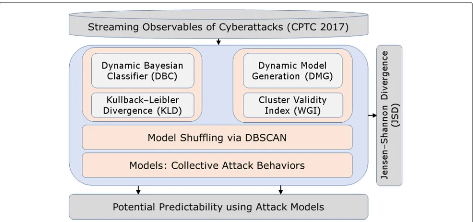
One may question the possibility to create attack models without ground truth of how cyberattacks progress, espe-cially with the evolving and situational nature of attack behaviors. ASSERT addresses these challenges by intro-ducing a semi-supervised Bayesian learning framework where the max-posteriors are converted to distances to the model centroid so as to assess and maximize the separation of models. More specifically, each aggregate of evidences (malicious activities occurring on the same source-target IP pair over a reasonable period of time) is either associated with the max-posterior attack model or used to generate a new model depending on which of the two gives a higher cluster validity index calcu-lated using the max-posterior distance. Attack models created will be continuously re-assessed as new evidences emerge. The aggregates of evidences may change over time and ASSERT ‘shuffles’ these aggregates through re-clustering when the cluster validity index is low. The occasional shuffling allows ASSERT to recover from early mis-association of evidences to models, while allowing continuous and computationally efficient Bayesian-based separation of evidences and synthesis of attack models. Figure1shows an overview of ASSERT architecture, along with its connection to experimental data and external assessment modules, in terms of both Jensen-Shannon Divergence (JSD) (Lin 1991) and potential predictability using the generated attack models.
The rest of the paper is organized as follows. “ Back-ground and related work” section summarizes the pre-vious works on extracting the intrinsic
spatiotempo-ral patterns in cyberattacks and classifying unlabeled and streaming network attack data. “Methodology: ASSERT” section gives the details of the ASSERT sys-tem including the use of dynamic Bayesian classi-fier with Kullback-Leibler divergence (KLD) (Kullback and Leibler 1951), model generation and assessment with Wemmert-Gancarski Index (WGI) (Wemmert et al. 2000), and shuffling with Density Based Spatial Clus-tering of Applications with Noise (DBSCAN) (Ester et al.1996). “Design of experiments” section presents the design of experiments, and “Results” section discusses the results to demonstrate ASSERT’s effectiveness in gener-ating quality attack models over time and its potential to improve prediction of future attack actions. Finally, “Conclusion” section presents concluding remarks as well as opportunities for future works.
Background and related work
The need to recognize different types of cyberattacks is not new. Early works created taxonomies of cyberat-tacks based on known attack strategies and compiled a list of categories that an attack can be associated with (Hansman and Hunt2005). Different taxonomies catego-rize cyberattacks based on various criteria e.g. the vul-nerability behind an attack or its observed consequences. These taxonomies serve the purpose to provide a founda-tional understanding of different types of attacks, allowing technical solutions to focus on detecting or differentiating specific attacks.
ASSERT aims at processing streaming intrusion alerts and separate observables of malicious events into empiri-cally generated attack models that can better differentiate attack behaviors and thus help predict future actions. Using a dynamic Bayesian approach, it focuses on group-ing intrusion alerts to create a collective behavior, not necessarily a similar one. This is different from many previous studies where similar observables are ‘clustered’ together to identify similar behaving end hosts (Xu et al. 2011) or traffic flows (McGregor et al.2004; Shadi et al. 2017; Song and Chen2007).
Fig. 1The ASSERT architecture and its connection to external modules
future actions. Past research works (Luo et al.2016) and (Bolzoni et al.2009) have suggested a similar concept and the need to integrate intrusion detection systems with attack classifiers.
There are several ways to model cyberattacks. Al-Mohannadi et al. provided an overview of some of the popular methods to model network attacks (Al-Mohannadi et al.2016) , and Yang et al. summarized a number of modeling approaches used for predicting future attacks (Yang et al.2014). One common approach used by many was using attack graphs to model the system vulnerabilities in a network and the inter-dependencies between these vulnerabilities. Also commonly referred to by the community has been the kill chain model that describes how an attack might progress as a chain of actions from reconnaissance, exploitation, lateral move-ments, evasions, etc. The Capability-Opportunity-Intent (COI) model characterizes cyberattacks based on the motif and capability of the attacker, the infrastructure of the network being attacked, and the defendability of the attacker (Salerno et al.2010). These modeling approaches (attack graphs, kill chain, and COI) have been used by many researchers to develop algorithms to correlate intru-sion alerts or to predict future attack actions. For example, Wang et al. proposed to use probabilistic attack graphs to correlate isolated alerts into attack scenarios, so as to effi-ciently identify the vulnerabilities that could be exploited in a network (Wang et al.2006; Wang et al.2010). Homer et al. discussed several methods to determine parts of an attack graph that would not help identify critical secu-rity threats and group similar attack steps as virtual nodes to increase the understandability of the data flow in a
network (Homer et al.68). Noel et al. introduced CyGraph as a tool for cyber warfare analytics which builds an attack graph model that maps the potential attack paths through a network (Noel et al. 2016). Aguessy et al. presented a Bayesian Attack Model (BAM) for dynamic risk assess-ment (Legany et al.2006). They combined the ideas of a topological attack graph and a Bayesian network in order to represent all possible attacks in an information sys-tem. The BAM approach aimed at associating possible attacks on a network with probabilities so that an analyst could identify the major vulnerabilities in the network. Shandilya et al. presented an overview of the state-of-the-art technologies in attack graph generation (Shandilya et al.2014).
studies shed lights on the spatial and temporal model-ing approaches that could capture cyberattack patterns from the attacker’s perspective. This research builds upon these foundations and develops a computationally effi-cient dynamic Bayesian approach with Kullback-Leibler divergence and entropy redistribution to process intru-sion alerts and create attack models in an online manner without a priori knowledge on either network topology or attack behaviors.
Traditional predictive analytics approaches require training data of known attacks which may not be easy to gather, due to the scarcity of the predictive indica-tors and the ground truth. Although some prior works use the observables of malicious activities reported by known global anti-virus programs as indicators (Yen et al. 2014; Bilge et al. 2017), most of the time it is difficult to gather the ground truth for a target. And without a priori or ground truth on the attack data, it is challenging to assess the quality of the generated empir-ical attack models. Are they similar? Will there be too many? Yen et al. state that they do not have ground truth for many aspects of their investigation, and use indi-rect indicators instead (Yen et al. 2014). A prior study (Liu et al. 2015) states that reported cybersecurity inci-dents that could serve as ground-truth are vastly under reported and uses the reported public incidents from the VERIS Community Database (VCDB) (VERIS2018), Hackmageddon (Hackmageddon 2018 and Web Hack-ing Incidents Database (WASC 2018). Bilge et al. state that obtaining labeled data that is sufficiently compre-hensive to capture all clean and risky host profiles in the wild is nearly impossible, because no malware detec-tion soludetec-tion can attain perfecdetec-tion due to the known arms-race with the cyber attackers (Bilge et al. 2017). When there is no labeled data, clustering could be used as an alternative unsupervised learning approach where similar instances are grouped together based on their attributes. Instances within the same cluster are expected to have a high similarity, whereas the instances of differ-ent clusters are expected to be dissimilar. A cluster validity index takes into account the separation between clus-ters along with the coherence of the data points within each cluster. Previous studies (Wang et al. 2009; Kovács et al.2005) have suggested the use of several cluster valid-ity indices to measure the qualvalid-ity of a clustering process. The concept of the cluster validity index coincides with the needs to assess the quality of the generated mod-els. This work, thus, adopts Wemmert-Gancarski Index (WGI) to complement the dynamic Bayesian approach to assess the quality of the generated and updated models regularly.
Classification of streaming data is a relatively new but growing problem. Streaming data is defined as data that enters the system one observable at a time. One common
method for the classification of streaming data is to use ensemble algorithms such as those described by Street and Kim (Street and Kim2001) and Kuncheva (Kuncheva 2008). These ensemble algorithms combine the results of multiple types of classifiers on a subset of the data stream. Another common practice for classifying stream-ing data is to store data points in memory until a large enough subset is gathered and then perform the clas-sification on these data chunks. The clasclas-sification can either be done using an ensemble algorithm or by cluster-ing (O’Callaghan et al.2002). Unlike the previous works, ASSERT is based on a novel Bayesian based model gen-eration approach which enables the classification of the streaming observables efficiently. The quality of the gen-erated attack models is regularly assessed with WGI and a systematic density based clustering approach is used to optimize earlier attack models.
Methodology: ASSERT
Intrusion alerts are commonly assessed by security ana-lysts with their statistics and statistical distributions. ASSERT uses a set of non-parameterized histograms that represent the statistically aggregated behavior as exhib-ited by the intrusion alerts. The non-parameterized his-tograms generalize the modeling approach for specific attack attributes, instead of assuming the attack behaviors are known a priori. Each set of histograms, for example, target IPs, target ports, alert categories, and alert signa-tures, is used to represent an attack behavior model that represents a set of potentially related malicious activi-ties. Intrusion alerts are first aggregated into ‘edges’ based on common source and target IP addresses. These edge-based aggregates will then be classified into an attack model that maximizes the posterior probability under the Bayesian framework, or used to create a new model. This work assumes that each edge-based aggregate in the same time proximity reflects an attack behavior. This assump-tion is reasonable since it is unlikely multiple attackers will use, or spoof, the same source IP to attack the same target IP in the same time frame without coordination. If there is coordination, the collective behavior is what ASSERT meant to capture. The aggregation enables the compari-son of non-parameterized histograms and thus generation of empirical models.
The overall process flow
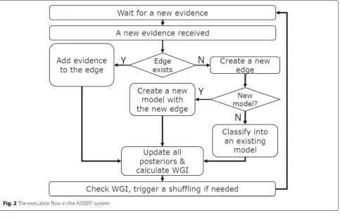
collective attack behavior exhibited by a specific combina-tion of intrusion signatures, port numbers,etc.. Each edge is represented by the non-parameterized histograms, and either matched to max-posterior attack model or used to create a new model if the histograms deviate too much from the existing models. As a subset of G, an attack model is a collection of edges and is represented by the histograms generated from the aggregated statistics of all edges within the model. Note that the empirically gener-ated models evolve over time since the edges added into a model contribute to the histograms associated with that model. This iterative process, as shown in Fig.2, allows the generation of empirical models without a priori knowl-edge of any specific attacks or network configuration.
When a new alert or evidencevis received, it is added to an existing edgeeon the overall graphGbetween the source and target IP addresses of the processed observ-able. Note that this graphGis not the same as the attack graph used in the literature; it is merely a representation of the collection of the edges. If no such edge exists, then it is created and added to the graph. The process of analyzing a new evidence is described in Algorithm 1.
Algorithm 1 Add evidencevto a new or existing edge ein an attack graphGwhere a dynamic attack model is represented by.
1: functionADDEVIDENCE(v, G)
2: ifaneforvdoes not exist inGthen 3: e=G.createEdge(v.sourceIP,v.targetIP) 4: formodelinGdo
5: e.updatePosterior()
6: classify(e,G) 7: else
8: e=G.getEdge(v.sourceIP,v.targetIP) 9: e.add(v)
10: G.updatePriors() 11: foredgeeinGdo
12: formodelinGdo
13: e.updatePosterior()
An edge e (an aggregate of evidences) may be classi-fied into an existing model or used to generate a new model. ASSERT adopts the use of Wemmert-Gancarski Index (WGI) to decide whether to create a new model. The inverse of the maximum posterior probability is con-sidered as the distance between each aggregate and the model centroid, and used to calculate WGI and determine the separation of the attack models. The WGI associ-ated with classifying a new edge to an existing model is compared to that associated with using the new edge to
generate a new model, and the decision goes to the one with the higher WGI. The process of deciding whether to create a new model or not is summarized in Algorithm 2.
Algorithm 2Classify an edgeeto a new modelnor an existing modele with maximum posterior fore in an attack graphGwhere[ ] represents the list of models.
1: functionCL ASSIFY(e, G) 2: if|[ ]| =0then
3: 0=G.createModel(e) 4: e.updatePosterior(0) 5: else
6: n=G.createModel(e) 7: WGIn =G.calculateWGI() 8: G.removeModel(n) 9: Findefore 10: e.setModel(e) 11: G.updatePriors() 12: foredgeeinGdo
13: formodelinGdo
14: e.updatePosterior()
15: WGIe=G.calculateWGI() 16: ifWGIn>WGIethen 17: e.remove(e)
18: G.createModel(e)
Dynamic Bayesian Classification
One of the key novelties of ASSERT is the calculation of P(X|)f that is the likelihood of a model generating an evidence aggregateX for a given featuref. Note that explicitly calculatingP(X|)f by assessing a large num-ber of combinatorial possible occurrences could lead to an extremely small likelihood, be computationally chal-lenging and cause precision errors in standard comput-ers. However, the use of a non-parametric histogram is needed, because there is no evidence in the community suggesting the target IP, port or exploit selections follow a certain distribution.
Given two probability distributions and X, the Kullback-Leibler divergence (KLD) (Kullback and Leibler 1951) is a non-symmetric measure of the difference betweenandX. It represents the amount of informa-tion lost when a modelis used to approximate an edge X. Therefore, instead of explicitly calculating P(X|)f, ASSERT uses KLD to estimate how well a model explains the observed evidences on an edge. Usingpias the prob-ability of a feature instanceiinandqias its probability inX, the KLD fromtoXfor a featuref is defined as
KLDf(X)=
i qilog
qi pi
Fig. 2The execution flow in the ASSERT system
ASSERT uses the inverse ofKLDto calculate the likeli-hood for each edge distributionX. Then, the likelihoods for all features are multiplied to find the overall likelihood between a modeland edgeX:
P(X|)= f
1 KLDf (X))+1
(2)
In addition, we recognize that it is not uncommon to have certain feature instances not show up in the model during the dynamic classification process. This can lead to zero probability when using KLD (which causes problem if anypi=0 in (1)). In the context of cyberattack modeling, not yet observing a feature instance (e.g. a specific exploit being used or a port being targeted) does not necessar-ily mean that such feature will not occur in the future. In fact, an attacker is likely to target different exploits, ports, and IPs over time. Therefore, ASSERT uses the Shannon’s entropy to estimate the stochastic nature of a feature his-togram and distribute the entropy to the unseen feature values in the model (), so as to reflect the possibility of having an unobserved feature instance.
More specifically, if a certain feature valueiis observed on an edge but is not seen in a model (pi =0), the Shan-non entropy of the feature model is used to calculate the probability of unseen feature observations in the model. The entropy of a feature f within a model i.e. Ef is calculated by
Ef = − n
i
pilog(pi) (3)
wherenis the total number of observations within the fea-ture histogram. ASSERT evenly distributes the entropy to all feature values, by definingpias
pi=pi
1−Ef
+|Ef
f| (4)
where 0 ≤ Ef ≤ 1 and|f|is the total number of feature values present in the model.
With this entropy re-distribution, ASSERT updates (1) by using pi instead ofpi. This gives the final likelihood for ASSERT, which is used in conjunction with a uniform prior and, in turn, determines the posterior between each pair of model and edge. The maximum posterior is then found and used to calculate WGI to determine whether to associate the edge to the max-posterior model or to use the edge to create a new model.
Dynamic model generation
creation of a new model. The choice between associating with an existing empirical model versus creating a new model is accomplished by treating the models as clus-ters, and the max-posterior as the inverse of the distance between an edge and its model.
If the posterior probability of an edgeXifor a model is represented byP(|Xi), the inverse of this posterior is defined as
di= 1 P(|Xi)
(5)
and is used as a distance metric to determine WGI cluster validity index. WGI is then used to assess the quality of the model separation, decide when a new model needs to be created, and trigger a new edge shuffling process. WGI defines a coherence and separation metricRfor each edge Xias
R(Xi)= di
mindi (6)
wheredirepresents the distance between an edgeXiand its max posterior model centroid anddi shows the dis-tance betweenXiand its second best model centroid. WGI takes the mean of R(Xi) for each model and defines a coherence and separation metricJkfor each model as
Jk=max
0, 1− 1 nk
nk
i R(Xi)
(7)
Jk takes the complement of the mean ofR(Xi)for model k to 1 (or ignore it when it is> 1) where nk shows the number of edges in modelk. Based on Eqs.6and7, WGI is defined as
WGI= 1
N N
k=1
nkJk (8)
where N represents the total number of models in the system. ASSERT uses nk = 1 in (8) in order to treat very large and relatively smaller models in the same way. This is needed particularly in the context of cyberattack modeling, because often times significant amount of the received alerts are scanning, and attack model generation should not be biased against non-scanning alerts.
Model shuffling via DBSCAN
ASSERT monitors the quality of the classification contin-uously by referencing the WGI. When WGI falls below a configurable threshold, a shuffling process is triggered to ensure that each edge is assigned to a model with the highest posterior and redundant models are removed. The shuffling process might be triggered several times throughout the execution flow based on the two trigger conditions:
1. Index Threshold (IT): If the WGI value falls below a
configured threshold.
2. Number of Evidences (ET): If the number of
evidences received after the last shuffle has reached a certain configured threshold.
To trigger a shuffling process, bothIT andET conditions must be satisfied. That means, ASSERT waits for a cer-tain number of evidences to trigger the shuffling, even if the index falls below the configured boundary to avoid a shuffling overhead.
ASSERT uses a density-based clustering algorithm i.e. DBSCAN that groups closely packed edges together. ASSERT uses DBSCAN, because unlike traditional clus-tering algorithms such ask-Means, it does not need to know the number of clusters, and can identify outliers if any. DBSCAN uses two parameters i.e. the epsilon () and the minimum number of points (mp) to define a dense region. The algorithm iterates through the edges that have not been visited and retrieves their-neighborhood. If the neighborhood contains enough number of edges a cluster is created, otherwise the edge is labeled as noise (outlier).
Note that DBSCAN requires pair-wise distances between edges. The pair-wise Jensen-Shannon divergence (JSD) is used as an estimate of the distance between edges, since there may not be sufficient evidences on the edges to determine the divergence. ASSERT uses the JSD, a symmetrized and smoothed version of the KLD, to calculate a distance matrix for the behavior aggregates (edges). Given two edges i.e.X1andX2, and a featuref, the JS divergence betweenX1andX2is calculated by
JSDf(X1X2)=π1KLDf(X1M)+π2KLDf(MX2) (9)
where π1 andπ2weights are calculated considering the number of evidences inX1andX2andM=π1X1+π2X2. Then the distance between two edges is found by
JSD(X1,X2)= 1 |f|
f
JSDf(X1X2) (10)
where|f|denotes the number of features.
ASSERT follows a systematic approach to set the param-eters of the DBSCAN algorithm. First, it uses the natural logarithm of the total number of edges to set the value of the mp parameter. Second, it computes the average distance of each edge to its k nearest neighbors, where k = mp. Then, these average distances are plotted in an ascending order and the elbow (knee) point on the plot is used to set the value of.
within these clusters as outliers. These outliers are not considered by DBSCAN as valid clusters, and thus not associated with any attack model. Note that an edge con-sidered an outlier by DBSCAN could contain the first observables of a unique and emerging attack behavior. Therefore, each of these edges should be given a chance to create a new model, or associated with the closest valid model. ASSERT reclassifies each of these outliers by either associating them to an existing regular cluster or creating a new model depending on the value of the WGI, which is the same process described in Algorithm 2.
Design of experiments
This paper demonstrates ASSERT’s capability using the intrusion alerts collected from the 2017 National Col-legiate Penetration Testing Competition (CPTC) (CPTC Organizing Committee 2017), where approximately 60 people from 10 teams attempting to penetrate into the same computing infrastructure to find as many vulnera-bilities as possible. Suricata was installed to capture mali-cious activities over approximately a 9-h period, and the Suricata alerts were used as inputs for the experiments shown in this paper (Suricata 2019). ASSERT processes the Suricata alerts one by one to generate and update empirical models without any a priori knowledge on either the attackers or the infrastructure. The source and target IPs are used to define the edges. In this set of experiments, alert category, alert signature, target IP, and target port are used as features to generate and refine dynamic attack models.
WGI and Jensen-Shannon divergence
ASSERT assesses the empirically generated models regu-larly using a cluster validity index. Clustering indexes are similar in nature, as they provide a measure for the intra and inter cluster quality. However, there might be differ-ences about what they need to calculate the index value. A key point for ASSERT is that there is no natural meaning of a behavior aggregate (edge) in a feature space. Because, an edge as characterized by multiple probability distribu-tion funcdistribu-tions, it may not have an easy interpretadistribu-tion of its distance to other edges. One key novelty of ASSERT is to interpret the model as the centroid and the posterior as the inverse of distance to the centroid during the Bayesian learning phase. Therefore, ASSERT uses the Wemmert-Gancarski Index (WGI) which treats the inverse of the calculated posterior as the distance to the model cen-troid, so as to reflect the intra-cluster compactness with the maximum a posterior and the inter-cluster separation with the second best posterior.
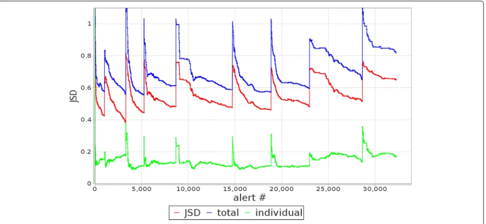
To provide an independent assessment of the quality of models generated, this work considers an alternative metric - the general Jensen-Shannon divergence (JSD). The general JSD is an extension of the pair-wise JSD
discussed in “Dynamic model generation” section, and aims at measuring the overall ‘divergence’ or coherence of multiple models. More specifically, the JSD of multiple models (1,2, ..n) based on a featuref is defined by the entropy of the combined model (ETf ) and the weighted average of individual model entropies (EfI).
JSDf(1,2, ..n)=ETf −EfI (11)
ETf =Ef( N
i=1
πii) (12)
EIf = N
i=1
πiEf(i) (13)
where πi represents the weight of a model i andN is the number of models. We use a uniform weight value of
πi = N1 for each model while calculatingEfT andEfI. It is desirable to have lower individual entropies (EIf) for bet-ter coherence within each model, and higher entropy for the combined model (EfT) for larger separation among the models.JSDf generates a value between 0 and log2N. For easy comparison over time whereNvaries, this work nor-malizes the general JSD of each feature by log2Nand then finds the average JSD over the multiple features by
JSD(1,2, ..n)= 1 |f|
f
JSDf. (14)
Predictability indices
ASSERT aims at generating and updating attack models, each reflecting a collective and unique behavior that could be used to enhance cyberattack prediction. If ASSERT is not used, the overall statistics from the cumulative intru-sion alerts i.e. all evidences from all edges in the entire graphGcould potentially be used by security profession-als to derive what might happen next. We will consider the statistical model from the entire graphGas the base-line. ASSERT focuses on how to best separate evidences of malicious activities in an online and robust manner. While there could be advanced cyberattack prediction algorithms (Fava et al.2008; Yang et al.2014), this work considers basic use of statistics to estimate the potential to predict which future actions might be observed. When a new evidence is received, ASSERT calculates the prob-ability of each feature value in the evidence, based on the model (that its edge is associated) versus that based on all the evidences in the graphG. This work considers this probability as an estimate of the potential ‘predictabil-ity’ that can be achieved for a given model or the overall statistics.
graphG. For the ease of presentation, we shall refer these probability values as the ‘predictability’ for the remain-der of this paper. The average predictability over a moving window is calculated and plotted to assess whether the generated model finds a better/higher probability of the imminent feature value compared to the baseline. More formally, the average predictabilities are calculated as
˜
pn()= 1 |w|
n
k=n−|w|+1
pki() (15)
˜
pn(G)= 1 |w|
n
k=n−|w|+1
pki(G) (16)
where|w|represents the size of the moving window andn shows the alert number.
Traditional cyber defense relies much on past obser-vations or statistics. The predictability metric presented above shows the potential value of ASSERT for all immi-nent feature values. What if a feature value never occurs on a given edge? This means predicting an ‘unseen’ fea-ture for a given source-target pair. If the generated model is effective, it should help to predict these unseen features better than using the overall graph. Note that the over-all graph has a larger sample size and potentiover-ally more likely to see a feature that are previously unseen on an edge. A model needs to be unique and useful for the edges associated with the model so as to have a higher pre-dictability for unseen features. This paper also compares the smoothed ‘unseen predictabilities’ (q˜n()andq˜n(G)) to assess whether ASSERT generates quality models that can help to predict the unseen features better.
Results
Before presenting the specific results, we summarize the parameters used for the set of experiments shown in this paper. ASSERT uses DBSCAN during shuffling with an
= 1.9 which reflects the elbow (or knee) point in thek-distance chart as explained in “Model shuffling via DBSCAN” section. A shuffling process is triggered each time when IT = 0.70 and ET = 1000. Moreover, a moving window size of 20 is used while calculating all pre-dictabilities i.e.p˜n(), p˜ni(G), q˜n() and q˜n(G). The IT andETparameters reflect user preference to tolerate over-all model quality (in WGI) versus processing time. They are used by ASSERT to decide when to trigger a shuffling process, which takes a longer time than a single Bayesian classification step but can re-assess the cumulative evi-dences at once. Selecting a higherIT or a lowerET will potentially lead to more shuffling processes and increase the total processing time for ASSERT but may give bet-ter WGI while evidences arrive, and vice versa.IT = 0.7 is chosen to ensure a relatively high quality of clustering throughout the execution process. A lowerIT could also
be chosen depending on the tolerance that the user has for the quality of the model separation or cohesion. Simi-larly, a higherET could be chosen, but that could mean a lower quality in WGI for a longer period of time. Depend-ing on the tolerance of the user for clusterDepend-ing quality, a higherET value might be selected.ET = 1000 is chosen as a threshold value for the CPTC’17 data set, to avoid fre-quent shufflings and wait for 1000 intrusion alerts before triggering a shuffling process when WGI is< 0.7. In our experiment, we observe that except the very first shuf-fling process,ETis not the dominating factor to trigger the shuffling processes. The iterative Bayesian classification performs reasonably well and thusITgoes below 0.7 after more than 1000 alerts are observed since last shuffling.
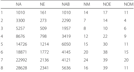
Processing 32,265 intrusion alerts in the CPTC17 data, ASSERT generates 2,392 edges and 47 attack models. Table1shows details of each shuffling process throughout the execution. ASSERT triggers a total of 8 re-clustering processes whereNAandNE show the cumulative num-ber of alerts and edges prior to each shuffling process. NABrepresents the number of alerts processed after the last shuffling andNMshows the number of models cre-ated at the end of each shuffling.NOEshows the number of edges in the outlier cluster generated by DBSCAN, and NOMrepresents the number of new models created from these edges. For example, 28628 alerts have been pro-cessed (5636 of which received after the 7thshuffling) and 2341 edges have been created prior to the 8th shuffling process. At the end of the 8thshuffling, a total of 16 models and 39 edge outliers were generated. 28 of these 39 outliers were associated to the 5 models generated by DBSCAN and the remaining 11 were used to create new models.
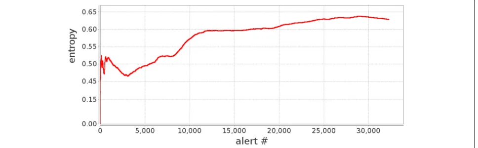
The CPTC17 data set includes a total of 20, 166, 68, and 495 distinct values for the alert category, alert signa-ture, target IP, and target port features, respectively. As the alerts come into the system, each of these features may see new values over time. Since an important chal-lenge for ASSERT is to associate edges with models even if some feature values exist in the model are not present on the edge, it is important to review the ‘entropy’ of the
Table 1Re-clustering processes for the CPTC17 data set
NA NE NAB NM NOE NOM
1 1010 161 1010 14 17 11
2 3300 273 2290 7 14 4
3 5257 509 1957 8 10 6
4 8676 798 3419 12 22 9
5 14726 1214 6050 15 30 11
6 18871 1772 4145 20 38 15
7 22992 2136 4121 24 39 20
features as the alerts come into the system. Figure3shows the average entropy of four features as more and more alerts come into the system. All four feature entropies fol-low similar trends, and thus not shown here. We observe that the average feature entropy fluctuates and has a gen-eral upward trend until it saturates after approximately 10,000 alerts are received. This observation coincides with the results in Table1, where more frequent shufflings are needed prior to the 10,000 alert mark.
The cluster validity index
As more edges are classified into a model, the collec-tive behavior of the model changes over time and it might not reflect the behavior of the edges classified into the model initially. Therefore, the overall separation and coherence of the generated models need to be moni-tored continuously. ASSERT assesses the quality of the empirically generated models regularly, using the WGI cluster validity index. The novel use of the inverse of the maximum posterior as a distance measure to the model centroids allows representing the intra-cluster compact-ness and the calculation of WGI in the absence of actual feature space (due to the complexity of non-parametric feature histograms). A decrease in WGI is possible, due to the divergence between the feature histograms of the edges and the model they are classified when additional evidences are observed on the edges. Therefore, a shuf-fling process using DBSCAN is used to re-cluster edges with the attack models. Figure 4 shows the change in the WGI as alerts come into the system. The number of steep rises in WGI, reflects the re-clustering processes triggered. While the re-clustering improves WGI, it takes on average 6.86 s to complete as opposed to only 0.11 milliseconds for each Bayesian classification. The com-bination of dynamic Bayesian classification and shuffling enables a good balance between computational efficiency to process streaming alerts and robustness to maintain quality models in terms of cohesiveness within each model and separations among them.
As shown in Table 1, NAB represents the number of alerts processed between two successive shuffling pro-cesses. This along with Fig. 4, shows more frequent shufflings occur prior to the 10,000 alert mark and less so later on. In fact, after the 8th shuffling, WGI did not come down and there was no need to shuf-fle. This trend somewhat coincides with the entropy shown in Fig. 3, where upward trend was observed until the 10,000 alert mark, and slight decline towards the end.
Jensen-Shannon divergence
Note that WGI shows the quality of the model in terms of the separation between the models and the cohesion within each model in the feature space. As an alternative and external measure to assess the quality of the gener-ated attack models, we calculate the general JSD among models as defined in “WGI and Jensen-Shannon diver-gence” section. Figure5 shows the general JSD (JSDf in (11) with the middle red line), the entropy of the com-bined model (ETf in (12) with the top blue line), and the average individual model entropy (EIf in (13) with the bot-tom green line). Note that the entropy of the combined model reflects the overall uncertainty (separation) across the individual models, and, thus, the higher the better. At the same time, the lower individual model entropy reflects better cohesion within each model. Overall, Fig.5shows that ASSERT performs well and have highETf and lowEIf. WhenETf become low, the shuffling triggered by WGI re-associates the edges with models and recoversETf without increasing too much on EfI (or have it go down quickly afterward with the dynamic Bayesian classifier).
Predictability
ASSERT associates an aggregated edge histogram to an attack model, expecting that the future behavior on the edge would be similar to its maximum posterior model. Therefore, if the classification of the attack behaviors
Fig. 4WGI over iterations with shuffling
is good, then the model statistics should be indicative of the feature values observed on an edge whether or not such features have occurred before on the edge. This section shows p˜n() and p˜ni(G) as defined in “Predictability indices” section and the next section dis-cusses the unseen predictabilities.
Recall that this paper defines ‘predictability’ as the like-lihood of a feature value as given by the attack model it is associated with, just before the feature value was observed. Note that advanced prediction algorithms e.g. (Fava et al. 2008) may take past transitions and other factors into account and likely achieve better prediction accuracy. The definition of predictability presented in this
paper is meant to assess the value of the attack models generated by ASSERT when used to predict next actions based on zero-order statistics. ASSERT is compared to the baseline where the cumulative statistical model is used to determine the likelihood.
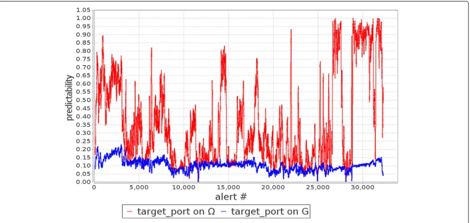
Figures 6, 7, 8 and9 showp˜n() andp˜ni(G) as alerts come into the system for the target IP, target port, alert signature and alert category features, respectively. Over-all, p˜n() clearly outperforms p˜ni(G) consistently over the entire dataset, showing the attack models created by ASSERT provide outstanding value for predicting future attack action features. To quantify this performance improvement, we define a predictability ratio (fn) =
Fig. 6Thep˜n()andp˜n(G)for target IP as the alerts come into the system
pni()/pni(G) for each feature f. It is observed that the average(fn)for the target IP, target port, alert signature, and alert category features are 12.80, 3.64, 2.39, and 4.39, respectively.
To compare the predictability measures in more detail, we calculate the percentage of times thepni()andpni(G) predictabilities are larger than a certain thresholdT, rang-ing between 0.05 and 0.5. Table2shows these percentages for all four features. Note that these are based on the indi-vidual probabilities while the lines plotted in the Figs.6,
7, 8 and 9 are based on the moving window average. Except the only case where the threshold is 0.05 for the target port feature, pni() exceeds the threshold signifi-cantly more often thanpni(G). This gap tends to increase as the threshold increases as well. This is interesting in that, it shows ASSERT is able to produce attack models that are capable of predicting specific feature values with much higher probabilities. For instance, the attack mod-els give a probability value of 0.35 or above for target IP 40.34% of the time while the cumulative statistics is at
Fig. 8Thep˜n()andp˜n(G)for alert signature as the alerts come into the system
0.01%. Similar performance gaps are observed for target port and alert signature at the same threshold level. There are much fewer number of unique alert categories, so it is relatively easier to predict, but similar performance gap is also observed at the threshold level of 0.5.
Unseen predictability
Similar to the analysis for the overall predictability, the probabilitiesq˜n()andq˜n(G), are calculated for each fea-ture instance that has never been seen on an edge. It
should be noted that these probabilities are calculated only if a feature instanceihas not been seen on its edge, but was seen in the associated model. Understandably, there are much fewer (but still significant) instances of unseens than the cases tracked in the previous section. For this section, we focus on the target port and alert signa-ture feasigna-tures because these two feasigna-tures have a significant number of distinct values (495 and 166, respectively) than the target IP (68) and alert category (20). Having more dis-tinct values means that there are more cases of unseens
Table 2The percentage of timespn
i() >Tandpni(G) >Tfor different features
Target IP Target port Signature Category
T pni() pni(G) pni() pni(G) pni() pni(G) pni() pni(G)
0.05 60.25 29.38 71.71 72.13 63.15 58.03 81.08 80.31
0.10 55.62 21.66 59.13 42.46 48.23 28.51 76.08 72.79
0.15 48.71 9.03 44.51 19.68 42.14 19.03 71.68 59.31
0.20 44.18 2.17 41.61 10.08 39.85 9.98 63.56 43.02
0.25 41.35 1.33 32.38 1.83 30.72 1.79 57.77 34.32
0.30 41.03 0.14 30.33 0.21 28.81 0.21 57.3 33.15
0.35 40.34 0.01 29.65 0 28.29 0 56.44 30.71
0.40 39.81 0.01 29.12 0 27.9 0 53.32 20.75
0.45 39.47 0 28.74 0 27.66 0 41.66 1.95
0.50 38.34 0 27.35 0 26.91 0 35.16 0
and it is harder to predict these values. Moreover, there is no ‘unseen’ instances of target IP based on our definition, since all target IPs seen in a model must already exist on an edge in the model. Note that predicting a potentially new target IP is an interesting research question, but is beyond the scope of this paper.
In order to have a set of previously observed evidences to check against, sufficient number of evidences must be processed by the system beforehand. Therefore, this paper reports the predictabilities for the unseen feature instances after the first 200 alerts come into the system. Figures 10and11 showq˜n() andq˜n(G) for the target port and alert signature features, respectively, as the alerts come into the system. Except very few cases, most of the timeq˜n()is higher thanq˜n(G). Note that the range
(y-axis) of unseen predictabilities is at around or below 0.1, much smaller than the cases presented in Figs.6,7,8and 9. This is expected, but also means that a more complex and careful design of prediction algorithms will be needed to leverage these lower zero-order probabilities.
We again use a set of probability thresholds (T) between 0.05 and 0.50 and count the percentage of times the unseen predictability measuresqni()andqni(G)are above these thresholds. Table 3 shows these percentages for the target port and alert signature features. As expected, ASSERT performs better than using the cumulative statis-tics to predict the unseens. In fact, using the cumulative statistics cannot produce any probabilities above 0.20 for unseen target port or alert signature features, while it is still feasible using ASSERT even at 0.50 level. Recall
Fig. 11q˜n()andq˜n(G)over iterations for the signature
again that the results shown in Table3are based on the individual probabilities while the plotted lines shown in Figs.10and11are based on the moving average, hence appears lower. Certainly, the benefits seem to be smaller than the overall cases presented in Table2. In fact, the average of the predictability ratio(fn) = qni()/qni(G) for the unseen target port and signature features are 1.17 and 1.22, respectively, which are much smaller than those reported for the overall predictability cases. This smaller performance gain is expected, since predicting unseens is fundamentally a daunting task. The fact that the attack models created by ASSERT can continuously produce sufficiently large probabilities for the unseens through-out the approximately 9-h CPTC event is promising. A careful design of a prediction algorithm that leverages these zero-order probabilities could potentially lead to an unprecedented capability where unseen attack actions can be actually predicted.
Attack models: a closer look
The core value of ASSERT lies in the creation of attack models that could assist the analysts to focus on critical activities and use such more targeted analysis to predict likely attack actions. In addition to the overall predictabil-ity analysis discussed in the previous sections, this section shows two attack models extracted from the same data set and describes how an analyst might be able to use them for insightful and targeted analysis. Specifically, we will show that each of these two attack models contains related attack actions from different teams and suggests attack actions that could possibly be executed by some teams, because another team or two in the same model has done them.
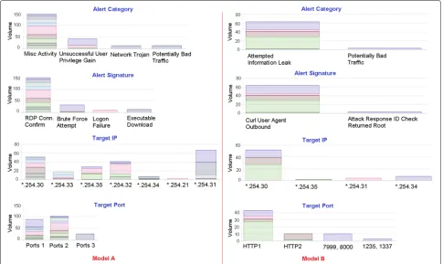
Figure12 shows the feature histograms of two attack models, Model A (left), which contains a total of 223 intru-sion alerts and a smaller Model B (right), which contains 65 alerts. As a reference, recall there are a total of 32,265 alerts in our data set. For each model, the feature his-tograms for the alert category, alert signature, target IP, and target port are provided. As stated earlier, the CPTC 2017 data set is composed of intrusion alerts from ten dif-ferent teams which are trying to penetrate into the same computing infrastructure. Therefore, each attack model includes intrusion alerts from various teams, and in each histogram alerts from different teams are represented with different colors.
Attack Model A aggregates potentially related intru-sion alerts from nine different teams and indicates a
Table 3The percentage of timesqni() >Tandqni(G) >Tfor the target port and alert signature features
Target port Signature
T qn
i() qni(G) qni() qni(G)
0.05 26.51 25.17 22.05 18.88
0.10 12.97 9.8 6.08 3.22
0.15 4.88 3.44 3.61 2.77
0.20 3.46 1.49 2.59 1.23
0.25 1.29 0 0.86 0
0.30 0.7 0 0.41 0
0.35 0.53 0 0.3 0
0.40 0.38 0 0.14 0
0.45 0.34 0 0.12 0
Fig. 12Alert category, alert signature, target IP and target port feature histograms for Models A (left) and B (right) generated by ASSERT. Thexandy
axis of each histogram show the individual feature values or categories and the number (volume) of alerts, respectively. Different colors in each bar represent alerts coming from the different teams
serious network trojan injection. Its alert category his-togram includes miscellaneous activity, unsuccessful user privilege gain, trojan detection, and potentially bad traf-fic categories. Its alert signature histogram indicates Remote Desktop Protocol (RDP) connection confirma-tions, potential FTP brute force attempts, repeated logon failures and executable script downloads. Similarly, its target port histogram includes alerts with categorized destination ports that are used by the Remote Desktop Management interfaces and its target IP histogram shows the victim IP numbers for the aforementioned exploits. The intrusion alerts of Model B are from five different teams, representing a collective attack behavior where the alert category histogram includes alerts for information leak attempts and potential bad traffic. The alert signature histogram shows executions of a critical command (curl) and the gain of critical ‘root’ privileges. The target port histogram shows related categorized ports through which the exploit was carried out and the target IP histogram shows the victim hosts.
We observe that each attack model aggregates poten-tially related exploits carried out by different attack teams. In Model A, all nine teams have RDP connection con-firmation alerts for a variety of target hosts. Team 6 has
RDP connection confirmation alerts for six different tar-get hosts, one of which is followed by a set of repeated logon failures. Similarly, Team 10 carries out a set of potential FTP brute-force attempts on a specific target, after a set of RDP connection confirmation alerts. There-fore, one might anticipate to see logon or FTP brute-force attempts executed by the remaining seven teams towards the target hosts for which an RDP connection confirma-tion alert is already observed. In Model B, five teams have used the command ‘curl’ to execute a data transfer. For one of these teams, intrusion alerts are observed showing that critical root privileges were gained. Therefore, one may anticipate a similar behavior from the remaining four teams towards the target hosts for which a ‘curl’ command is already executed.
merely show a potential use of ASSERT where the analysts can focus on a small number of critical alerts from vari-ous attack sources (different teams) and make prediction without being overwhelmed by the tens of thousands of alerts. The emerging threats exhibited through the empir-ical models do not require a priori knowledge and are adaptive as more evidences are collected.
Conclusion
In the absence of a priori knowledge on specific attacks and network configuration, ASSERT processes aggregated non-parametric feature histograms from streaming intru-sion alerts to generate attack models using a dynamic Bayesian approach with a novel likelihood calculation, regularly assessed with WGI, and complemented with DBSCAN. The key novelties of the ASSERT system are:
• The use of posterior as the inverse of distance to cluster centroid enables the integrated use of Bayesian classifier and WGI in a dynamic manner, as a foundation for the semi-supervised online learning framework that synthesizes cyberattack models.
• The use of KLD with entropy redistribution over non-parametric feature histograms enables the association of observable aggregates with empirical models even if there are emerging features that are previously unseen.
• The use of pair-wise JSD between observable aggregates allows re-clustering with DBSCAN, which enables improvement and recovery from imperfect decisions made earlier by the dynamic Bayesian classifier with insufficient evidences.
Using the intrusion alerts from the 2017 CPTC data set, this paper demonstrates the capability of ASSERT in generating and updating distinct attack models over time without a priori knowledge. Using WGI and gen-eral multi-model JSD, we show that both the cohesive-ness within individual models and the separation between models remain sound as new alerts are received. These models are also shown to be promising in predicting future attack actions. In particular, we assess the ‘pre-dictability’ against the baseline using total cumulative statistics, a reasonable practice in reading intrusion alert data. ASSERT is able to produce probabilities that are 12.80, 3.64, 2.39, and 4.39 times higher than the baseline on average for the target IP, target port, alert signature, and alert category respectively. Furthermore, it is able to predict unseen target port and alert signature with prob-ability values over 0.25 or even 0.5 while the baseline cannot produce any over 0.20. These results demonstrate the value of the attack models synthesized by ASSERT in predicting the ‘where’, ‘how’, and ‘what’ of future attack actions. Certainly, a careful design of how to use these models and feature predictions for an actual cyberattack
prediction is needed and underway. This work demon-strates a clear and consistent advantage of using ASSERT to develop such a predictor.
The overall ASSERT framework and the experiment methodology presented in this paper are also generaliz-able for using additional features and assessing empiri-cal models. In addition to the novelties of ASSERT, the introduction of the general multi-model JSD and the com-prehensive evaluation using ‘predictability’ and ‘unseen predictability’ is important for the community as we move towards predictive cyber defense and in need of a way to assess empirical attack models without a priori knowl-edge.
ASSERT separates intrusion alerts into empirical attack models where the analysts may focus on critical activi-ties and use the aggregated statistics from selected models to potentially predict future attack actions. While the assumption of edge aggregates within a reasonable dura-tion is sound, there is a risk of adversaries intendura-tionally embedding one or two critical exploits into very large number of common scanning activities in some edges. In such cases, ASSERT could still reveal the critical exploits as part of the attack model, but they will be statisti-cally insignificant to derive a high predictability or the improvement in predictability would be limited. Another limitation of the current implementation of ASSERT is the inclusion of historical alerts, where the system needs to define how and when the alerts will be treated as part of historical instead of emerging attack behaviors. Finally, additional experiments with more engineered features as well as human subject study will be beneficial to maximize the value provided by the ASSERT framework.
Funding
This research is supported by NSF Award #1526383.
Availability of data and materials
The data used during this research will not be shared, because it is protected by a confidentiality agreement.
Authors’ contributions
AO: The lead researcher and author. SJY: Developed research ideas and helped in writing. All authors read and approved the final manuscript.
Competing interests
All authors declare that they have no competing interests.
Publisher’s Note
Springer Nature remains neutral with regard to jurisdictional claims in published maps and institutional affiliations.
Received: 16 January 2019 Accepted: 15 April 2019
References
Bilge L, Han Y, Dell’Amico M (2017) Riskteller: Predicting the risk of cyber incidents. In: Proceedings of the 2017 ACM SIGSAC Conference on Computer and Communications Security (CCS). ACM, New York. pp 1299–1311.https://doi.org/10.1145/3133956.3134022
Bolzoni D, Etalle S, Hartel PH (2009) Panacea: Automating attack classification for anomaly-based network intrusion detection systems. In: Kirda E, Jha S (eds). Recent Advances in Intrusion Detection. RAID 2009. Lecture Notes in Computer Science, vol 5758. Springer, Berlin, Heidelberg
Chen YZ, Huang ZG, Xu S, Lai YC (2015) Spatiotemporal patterns and predictability of cyberattacks. PLOS ONE 10(6):1–1.https://doi.org/10. 1371/journal.pone.0131501
CPTC Organizing Committee (2017) Collegiate penetration testing
competition at Rochester Institute of Technology.https://nationalcptc.org/
Du H, Yang SJ (2011) Discovering collaborative cyber attack patterns using social network analysis. In: Proceedings of the 4th International Conference on Social Computing, Behavioral-Cultural Modeling and Prediction. Springer Berlin Heidelberg, College Park. pp 129–136 Ester M, Kriegel HP, Sander J, Xu X (1996) A density-based algorithm for
discovering clusters a density-based algorithm for discovering clusters in large spatial databases with noise. In: Proceedings of the Second International Conference on Knowledge Discovery and Data Mining. AAAI Press, KDD’96. pp 226–231.http://dl.acm.org/citation.cfm?id=3001460. 3001507
Fava DS, Byers SR, Yang SJ (2008) Projecting cyberattacks through
variable-length markov models. IEEE Trans Inf Forensic Secur 3(3):359–369.
https://doi.org/10.1109/TIFS.2008.924605
Hackmageddon (2018) Hackmageddon information security timelines and statistics.http://www.hackmageddon.com/. Accessed 6 Feb 2018 Haddadi F, Khanchi S, Shetabi M, Derhami V (2010) Intrusion detection and
attack classification using feed-forward neural network. In: Proceedings of the 2010 Second International Conference on Computer and Network Technology, IEEE Computer Society, Washington, DC. pp 262–266.https:// doi.org/10.1109/ICCNT.2010.28. ICCNT ’10
Hansman S, Hunt R (2005) A taxonomy of network and computer attacks. Comput Secur 24(1):31–43
Homer J, Varikuti A, Ou X, Mcqueen MA (68) Improving attack graph visualization through data reduction and attack grouping. In: Proceedings of the 5th International Workshop on Visualization for Computer Security. Springer-Verlag, Berlin.https://doi.org/10.1007/978-3-540-85933-8_7
Kovács F, Legány C, Babos A (2005) Cluster validity measurement techniques. In: 6th International symposium of hungarian researchers on
computational intelligence
Kullback S, Leibler RA (1951) On information and sufficiency. Ann Math Stat 22(1):79–86. [https://doi.org/10.1214/aoms/1177729694]
Kuncheva LI (2008) Classifier ensembles for detecting concept change in streaming data: Overview and perspectives. In: 2nd Workshop SUEMA. pp 5–10
Legany C, Juhasz S, Babos A (2006) Cluster validity measurement techniques. In: Proceedings of the 5th WSEAS International Conference on Artificial Intelligence, Knowledge Engineering and Data Bases, World Scientific and Engineering Academy and Society (WSEAS) AIKED’06. Stevens Point, Wisconsin. pp 388–393
Li Y, Xia J, Zhang S, Yan J, Ai X, Dai K (2012) An efficient intrusion detection system based on support vector machines and gradually feature removal method. Expert Syst Appl 39(1):424–430. [http://doi.org/10.1016/j.eswa. 2011.07.032]
Lin J (1991) Divergence measures based on the shannon entropy. IEEE Trans Inf Theory 37:145–151
Liu Y, Sarabi A, Zhang J, Naghizadeh P, Karir M, Bailey M, Liu M (2015) Cloudy with a chance of breach: Forecasting cyber security incidents. In: 24th USENIX Security Symposium (USENIX Security 15). USENIX Association, Washington, D.C. pp 1009–1024
Luo G, Wen Y, Lingyun X (2016) Network attack classification and recognition using hmm and improved evidence theory. Int J Adv Comput Sci Appl 7(4) McGregor A, Hall M, Lorier P, Brunskill J (2004) Flow clustering using machine
learning techniques. In: Pratt I, Barakat C (eds). Passive and Active Network Measurement. Springer Berlin Heidelberg, Berlin. pp 205–214
Ning P, Xu D, Healey CG, Amant RS (2004) Building attack scenarios through integration of complementary alert correlation methods. In: Proceedings of the 11th Annual Network and Distributed System Security Symposium. pp 97–111
Noel S, Harley E, Tam K, Limiero M, Share M (2016) Chapter 4 – CyGraph: Graph-based analytics and visualization for cybersecurity. In: Gudivada VN,
Raghavan VV, Govindaraju V, Rao C (eds). Cognitive Computing: Theory and Applications, Handbook of Statistics, vol 35. Elsevier. pp 117–167.
https://doi.org/10.1016/bs.host.2016.07.001
O’Callaghan L, Mishra N, Meyerson A, Guha S, Motwani R (2002)
Streaming-data algorithms for high-quality clustering. In: Proceedings of the 18th International Conference on Data Engineering. pp 685–694.
https://doi.org/10.1109/ICDE.2002.994785
Salerno JJ, Yang SJ, Kadar I, Sudit M, Tadda GP, Holsopple J (2010) Issues and challenges in higher level fusion: Threat/impact assessment and intent modeling (a panel summary). In: 2010 13th International Conference on Information Fusion.https://doi.org/10.1109/ICIF.2010.5711862
Shadi K, Natarajan P, Dovrolis C (2017) Hierarchical ip flow clustering. In: Proceedings of the Workshop on Big Data Analytics and Machine Learning for Data Communication Networks. ACM, New York Big-DAMA ’17. pp 25–30.http://doi.acm.org/10.1145/3098593.3098598
Shandilya V, Simmons CB, Shiva S (2014) Use of attack graphs in security systems. J Comput Netw Commun:13.http://doi.org/10.1155/2014/818957
Song S, Chen Z (2007) Adaptive network flow clustering. In: Proceedings of the IEEE International Conference on Networking, Sensing and Control, London. pp 596–601.https://doi.org/10.1109/ICNSC.2007.372846
Strapp S, Yang SJ (2014) Segmenting large-scale cyber attacks for online behavior model generation. In: Kennedy WG, Agarwal N, Yang SJ (eds). Social Computing, Behavioral-Cultural Modeling and Prediction. Springer International Publishing. pp 169–177
Street WN, Kim Y (2001) A streaming ensemble algorithm (sea) for large-scale classification. In: Proceedings of the Seventh ACM SIGKDD International Conference on Knowledge Discovery and Data Mining. ACM, New York KDD ’01. pp 377–382.https://doi.org/10.1145/502512.502568 http://doi. acm.org/10.1145/502512.502568
Subba B, Biswas S, Karmakar S (2016) A neural network based system for intrusion detection and attack classification. In: Proceedings of the National Conference on Communication (NCC).https://doi.org/10.1109/ NCC.2016.7561088
Suricata (2019) An open source-based intrusion detection system (ids).https:// suricata-ids.org/. Accessed 15 Jan 2019
Symantec (2017) Internet security threat report.https://www.symantec.com/ security-center/threat-report. Accessed 25 Apr 2017
Valeur F, Vigna G, Kruegel C, Kemmerer RA (2004) Comprehensive approach to intrusion detection alert correlation. IEEE Trans Dependable Secure Comput 1(3):146–169
VERIS (2018) Veris community database (vcdb).http://veriscommunity.net/ index.html. Accessed 6 Sept 2018
Wang K, Wang B, Peng L (2009) CVAP: validation for cluster analyses. Data Sci J 8:88–93
Wang L, Liu A, Jajodia S (2006) Using attack graphs for correlating, hypothesizing, and predicting intrusion alerts. Comput Commun 29(15):2917–2933.https://doi.org/10.1016/j.comcom.2006.04.001
Wang L, Jajodia S, Singhal A, Noel S (2010) k-Zero Day Safety: Measuring the Security Risk of Networks against Unknown Attacks. Springer Berlin Heidelberg, Berlin
WASC (2018) The web hacking incident database.http://projects.webappsec. org/w/page/13246995/Web-Hacking-Incident-Database. Accessed 6 Sept 2018
Wemmert C, Gan˙carski P, Korczak JJ (2000) A collaborative approach to combine multiple learning methods. Int J Artif Intell Tools 9(01):59–78 Xu K, Wang F, Gu L (2011) Network-aware behavior clustering of internet end
hosts. In: 2011 Proceedings of the IEEE INFOCOM. pp 2078–2086.https:// doi.org/10.1109/INFCOM.2011.5935017
Yang SJ, Stotz A, Holsopple J, Sudit M, Kuhl M (2009) High level information fusion for tracking and projection of multistage cyber attacks. Inf Fusion 10(1):107–121.https://doi.org/10.1016/j.inffus.2007.06.002
Yang SJ, Du H, Holsopple J, Sudit M (2014) Attack projection. In: Kott A, Wang C, Erbacher RF (eds). Cyber Defense and Situational Awareness. Springer International Publishing, New York City, chap Attack Projection. pp 239–261 Yen TF, Heorhiadi V, Oprea A, Reiter MK, Juels A (2014) An epidemiological
study of malware encounters in a large enterprise. In: Proceedings of the 2014 ACM SIGSAC Conference on Computer and Communications Security (CCS). ACM, New York, CCS ’14. pp 1117–1130.https://doi.org/10. 1145/2660267.2660330