A HOT-WIRE ANEMOMETER FOR PARTICLE COUNTERS
by
Nicholas H. Terrell
A thesis
submitted in partial fulfillment of the requirements for the degree of Master of Science in Computer Engineering
Boise State University
BOISE STATE UNIVERSITY GRADUATE COLLEGE
DEFENSE COMMITTEE AND FINAL READING APPROVALS
of the thesis submitted by
Nicholas H. Terrell
Thesis Title: A Hot-Wire Anemometer for Particle Counters Date of Final Oral Examination: 15 December 2014
The following individuals read and discussed the thesis submitted by student Nicholas H. Terrell, and they evaluated their presentation and response to questions during the final oral examination. They found that the student passed the final oral examination.
Sin Ming Loo, Ph.D. Chair, Supervisory Committee John N. Chiasson, Ph.D. Member, Supervisory Committee Donald Plumlee, Ph.D. Member, Supervisory Committee
ACKNOWLEDGEMENTS
I would like to thank my wife Michelle for her unending support. Her ability to maintain patience with both my work and her work has been the key to my success.
I would like to thank Dr. Sin Ming Loo for giving me the opportunity to exceed beyond my expectations. His guidance and mentorship have proven to be invaluable through the course of my work. I would also like to thank the members of the Hartman System Integration Lab for their work on the Personal Monitoring system and friendship.
I would like to thank my committee, Dr. John Chiasson and Dr. Don Plumlee, for their help and their time. Lastly, I would like to thank Dr. Jim Hall for his continuous help regarding the particle counter.
ABSTRACT
A Hot-Wire Anemometer for Particle Counters Nicholas H. Terrell
Master of Science in Computer Engineering
Portable real-time air quality monitoring is becoming a reality. While the data quality of these devices may be questionable, they have shown to be promising. One such device is the optical particle counter. The particle counter functions by having laminar airflow with constant velocity traverse the path of a laser beam within an airflow channel. This thesis presents the design and integration of a hot-wire anemometer into the flow channel. The addition of an anemometer allows for real-time airflow velocity
measurements to be performed and adjusted. Data from the anemometer can also be used to directly offset irregularities in particulate measurements during flow speeds outside the corrective capabilities of the fan. Experimental results show that an integrated
anemometer is capable of correcting varying external disturbances and improving the accuracy of particle counting measurements.
TABLE OF CONTENTS
ACKNOWLEDGEMENTS ... iv
ABSTRACT ... v
LIST OF TABLES ... x
LIST OF FIGURES ... xi
LIST OF ABBREVIATIONS ... xiv
CHAPTER 1: INTRODUCTION ... 1
1.1 Optical Particle Counters ... 1
1.2 Hot-Wire Anemometers ... 4
1.3 Motivation ... 5
1.4 Contribution ... 6
1.5 Work Overview ... 6
1.6 Outline... 7
CHAPTER 2: PREVIOUS RESEARCH AND EXISTING TECHNOLOGY ... 8
2.1 Previous Research ... 8
2.1.1 PMON Motherboard ... 9
2.1.2 Airflow Channel... 11
2. 1. 3 Firmware and Software ... 14
2.2 Existing Technology ... 14
2.2.1 Optical Particle Counters ... 14
2.2.2 Hot-Wire Anemometers ... 18
CHAPTER 3: OPTICAL PARTICLE COUNTER ... 20
3. 1 Overview of Optical Particle Counting... 20
3.1.1 OPC Design ... 20
3.1.2 OPC Calibration ... 21
CHAPTER 4: HOT-WIRE ANEMOMETER ... 27
4.1 Theory ... 27
4.2 Constant Current Anemometer (CCA) ... 30
4.3 Constant Temperature Anemometer (CTA) ... 32
4.4 Constant Voltage Anemometer (CVA) ... 33
CHAPTER 5: HARDWARE DESIGN ... 35
5.1 Anemometer Probe ... 35
5.1.1 Wire Resistance Estimation ... 35
5.1.2 Probe Design and Implementation ... 37
5.1.3 Results ... 40
5.2 Constant Current Anemometer ... 40
5.2.1 CCA Simulation ... 41
5.2.2 CCA Design ... 43
5.2.3 CCA Results... 45
5.3 Constant Temperature Anemometer ... 46
5.3.1 CTA Simulation ... 46
5.3.2 CTA Design ... 47
5.3.3 CTA Results ... 49
CHAPTER 6: FIRMWARE DESIGN ... 51
6.1 Optical Particle Counter Firmware ... 51
6.1.1 Original Counting Method ... 51
6.1.2 Effects of Varying Airflow on Particle Counts... 54
6.1.3 Particle Count Compensation ... 58
6.2 Hot-Wire Anemometer Firmware ... 61
6.2.1 Sensor Framework ... 62
6.2.2 Probe Resistance ... 65
6.2.3 Reference Voltage ... 67
6.2.4 Anemometer Calibration ... 70
6.2.5 Airflow Conversion ... 71
6.3 Fan Control System... 74
6.3.1 Airflow Velocity and PWM Relationship... 75
6.3.2 Controller Calibration ... 76
CHAPTER 7: TESTING AND RESULTS... 79
7.1 Anemometer Verification ... 79
7.2 Fan Control Results... 80
7.3 OPC Compensation Results ... 83
CHAPTER 8: CONCLUSION AND FUTURE WORK ... 86
8.1 Conclusion ... 86
8.2 Future Research ... 86
8.2.1 Optical Particle Counter ... 86
8.2.2 Hot-Wire Anemometer ... 87
8.2.3 Integrated System... 89 REFERENCES ... 91
LIST OF TABLES
Table 1: Resistance Estimation Results during Anemometer Initialization... 67
LIST OF FIGURES
Figure 1: Optical Particle Counting Cross Sectional View (1) Laser Source; (2) Light Blocks; (3) Particulate and Photodiode; (4) Laser Termination
Point ... 3
Figure 2: EXTECH Instruments Hot-Wire Thermo Anemometer with Datalogger Model SDL350, where (A) is the Probe, (B) is the Datalogger and Heating Circuit, and (C) are the Probe Leads [8]... 5
Figure 3: Zoomed View of EXTECH Probe ... 5
Figure 4: Full PMON Unit, Top Removed ... 8
Figure 5: PMON OPC Flow Channel and Enclosure ... 11
Figure 6: Fan Control Block Diagram ... 12
Figure 7: PMON OPC Airflow Channel Showing Direction of Flow (Blue) and Incident Laser Beam (Red) ... 13
Figure 8: Dylos DC1100 Air Quality Monitor [14] ... 17
Figure 9: Particle Generation System and Chamber Used for OPC Calibration [6] ... 23
Figure 10: External Airflow Disturbance Test in OPC Calibration Chamber ... 25
Figure 11: External Airflow Disturbance Test Results ... 26
Figure 12: CCA Circuit [15]... 31
Figure 13: CTA Circuit [15] ... 32
Figure 14: CVA Circuit [15] ... 34
Figure 15: Estimation of Temperature for Resistances of Tungsten Wire ... 37
Figure 16: (a) Probe Layout for the OPC Flow Channel, (b) Probe Layout for the Test Channel, (c) Actual OPC Probe, (d) Actual Test Probe ... 38
Figure 17: LTSpice CCA Circuit Simulation ... 41
Figure 18: LTSpice CCA Simulation Voltage Output over Wire Resistance ... 42
Figure 19: CCA Eagle Schematic... 44
Figure 20: CCA Output Voltage as a Function of Airflow Velocity ... 45
Figure 21: LTSpice Simulation of the Basic CTA Circuit ... 46
Figure 22: CTA Eagle Schematic Excluding DAC, ADC, and FFC Headers ... 48
Figure 23: CTA Feedback Voltage as a Function of Airflow Velocity ... 49
Figure 24: Operating Feedback Voltage at No Flow Conditions as a Function of Probe Starting Resistance ... 50
Figure 25: Simplified Particle Processing Algorithm Flowchart ... 52
Figure 26: Particle Count Sample Scaling Flowchart ... 53
Figure 27: Effects of Varying Airflow on Particulate Measurements ... 55
Figure 28: Effects of Varied Airflow Velocities on Average Particle Pulse Amplitude ... 56
Figure 29: Effects of Varied Airflow Velocities on Average Particle Pulse Duration ... 57
Figure 30: Reynolds Number for Varied Airflow Velocities at 3 Operating Temperatures... 58
Figure 31: Particle Processing Compensation Flowchart ... 59
Figure 32: Sample Scaling Compensation Flowchart ... 60
Figure 33: Pulse Height Error due to Increased Airflow Velocities ... 61
Figure 34: CTA Initialization Flowchart ... 63
Figure 35: Anemometer Sensor Task Flowchart ... 64
Figure 36: Sensor Interval Flowchart ... 64
Figure 37: Initial Wire Resistance Measurement Flowchart ... 66
Figure 38: Feedback Voltage of Airflow for Highly Resistive Probe (6.5𝛀)
with DAC Output of 1V ... 68 Figure 39: Feedback Voltage of Airflow for Highly Resistive Probe (6.5𝛀)
with DAC Output of 1.4V ... 69 Figure 40: CTA Calibration Using n = 0.2 ... 71
Figure 41: Airflow Conversion Flowchart ... 73 Figure 42: Relationship between Anemometer Feedback Voltage and Ambient
Temperature ... 74 Figure 43: Alternate Fan Control Loop with Integrated Hot-Wire Anemometer ... 75 Figure 44: Airflow Velocity as a Result of PWM Duty Cycle High Time ... 76 Figure 45: Comparison of Measurements from Calibrated Test Probe
and EXTECH Model... 80 Figure 46: Effects of External Pressure and Flow Variations on PMON
Internal Airflow Velocity ... 81 Figure 47: Airflow Velocity during Assisted Airflow Controller Response ... 82 Figure 48: Airflow Velocity during Conflicted Airflow Controller Response ... 82 Figure 49: Comparison between Airflow Velocity and Particle Concentration
Measurements after Compensation. ... 84
LIST OF ABBREVIATIONS
ADC Analog-to-Digital Converter ARM Advanced RISC Machine CFM Cubic Feet per Minute
CPC Condensation Particle Counter DAC Digital-to-Analog Converter
DC Direct Current
DMM Digital Multi-Meter EMF Electromotive Force
EPA Environmental Protection Agency FAA Federal Aviation Administration
HSIL Hartman System Integration Laboratory I2C Inter-Integrated Circuit
ISR Interrupt Service Routine LAN Local Area Network
MEMS Microelectromechanical Systems OPC Optical Particle Counter
PCB Printed Circuit Board PI Proportional-Integral
PID Proportional-Integral-Derivative PM Particulate Matter
PMON Personal Monitor PPL Particles per Liter PWM Pulse Width Modulation RC Resistor-Capacitor
RF Radio Frequency
RISC Reduced Instruction Set Computer RPM Rotations per Minute
SD Secure Digital SLA Stereo Lithography SNR Signal-to-Noise Ratio SPI Serial Peripheral Interface SPOS Single Particle Optical Sensing
TCP/IP Transmission Control Protocol/Internet Protocol TEOM Tapered Element Oscillating Microbalance UART Universal Asynchronous Receive/Transmit USB Universal Serial Bus
WHO World Health Organization
CHAPTER 1: INTRODUCTION
In recent years, the public is finding that air quality plays a vital role in the health of those exposed [1-4]. Yet, real-time monitoring remains largely inaccessible to the vast majority of the public. In order to facilitate this growing need for environmental air quality data, portable sensing systems have seen an increase in research and development. Among many of the various sensors, airborne particulate measuring devices remain one of the more difficult to develop. Factors such as cost, cross sensitivities, and battery life all play very important roles in a portable system. One method to reduce cost and prolong battery life is to use an axial fan instead of a pump. However, maintaining constant airflow characteristics (e.g., velocity) with a fan can be complicated. In this research, a fan-based particle counter is augmented with a hot-wire anemometer. Airflow velocity can be detected and then be used to vary the fan’s rotational speed. With this addition, particulate measurements, such as counts or sizes, can be more accurately determined with airflow measurements.
1.1 Optical Particle Counters
By the 1970s, the link between cardiopulmonary diseases and airborne pollutants in the form of particulate matter (PM) became generally acknowledged amongst
consequence, airborne particulate matter has become increasingly studied in recent years [3].
The findings of the research performed in the last decade have continuously shown a general negative impact on human health in regions with certain PM characteristics. For example, the World Health Organization (WHO) estimates that airborne PM2.5 is the source for an estimated 500,000 premature deaths every year [2]. A 2004 study shows possible connections between inflammation, coagulation, and heart rhythms in healthy younger men exposed to ambient, in-car and roadside PM [4]. Even simple in-door dust is capable of ranging from millimeters to nanometers in size and has been shown to increase the risk for developing cardiovascular and lung diseases [1].
Unfortunately, understanding the nature of particulates can be difficult. Air pollution monitoring generally requires expensive equipment and facilities not available to the average consumer. Thus, knowing what events generate harmful particulates and how the surrounding environment is impacted is made a difficult task. As a result, the Environmental Protection Agency (EPA) has shown great interest in the development of low-cost, real-time air monitoring technologies [5].
and size. Figure 1shows the basic concept of a scattering-based OPC. The laser rests on one side of the flow channel and emits a beam orthogonal to the particulate flow.
Figure 1: Optical Particle Counting Cross-Sectional View; (1) Laser Source; (2) Light Blocks; (3) Particulate and Photodiode; (4) Laser Termination Point
A series of light blocks protects the photodiode from errant light splashes potentially caused by the laser beam. The particulate, shown in (3) of Figure 1, crosses the beam and causes light to scatter towards the photodiode. The beam enters the
termination point and is prevented from reflecting back into the flow channel. One should note that the particulate size and beam shape in Figure 1 are not to scale and have been exaggerated for clarity.
Portable OPCs require air sampling either through the use of a fan or a pump [6]. Pump-driven OPCs have the advantage of a consistent airflow velocity through the flow channel but are noisy and costly. Given that these devices are designed for use in many environments, noise pollution in home and workplaces may be deemed unacceptable.
blockages or external pressure variations) affecting the airflow. In order to track the actual airflow velocity in real-time, a sensor (such as a hot-wire anemometer) should be placed within the channel. The measurements can then be used to alter the fan’s RPM set point to provide more or less airflow velocity. If the effects of airflow velocity on particle counts and measurements are characterized, then the results from the anemometer can also be used to enhance the overall accuracy of the particle counter.
1.2 Hot-Wire Anemometers
A hot-wire anemometer is a sensor capable of sampling subsonic or supersonic fluid flow velocities. Hot-wire anemometers generally consist of a micrometer thick wire, temperature control circuitry, and data acquisition circuitry. The wire can be installed inside a flow channel or a probe. The probe of the anemometer is then placed at the location where an airflow velocity measurement is desired. Probes are usually separated from the anemometer’s heating circuitry and connected by leads. In some anemometer designs, the probe is part of small handheld rod as shown in Figure 2 and Figure 3. In other anemometers, the probe may only be an enclosure used to support the wire. The wire is made of a material that can withstand high temperatures without corroding.
By having airflow around the wire, convective heat transfer cools the wire,
Figure 2: EXTECH Instruments Hot-Wire Thermo Anemometer with Datalogger Model SDL350, where (A) is the Probe, (B) is the Datalogger and
Heating Circuit, and (C) are the Probe Leads [8].
Figure 3: Zoomed View of EXTECH Probe
1.3 Motivation
to be lowered. OPCs can be made available in vehicles, homes, offices, and outdoor environments without an obtrusive presence. Ideally, little to no maintenance should be required to keep the OPC functional and accurate.
Wind gusts are common in the outdoors environment and can have drastic effects on airflow velocity and PM measurements. Portable OPCs are also expected to be on the move while collecting data. Movement velocities of high enough intensity can generate air resistance, changing the pressure levels around the inputs and outputs of the flow channel. By outfitting an OPC with a hot-wire anemometer, the OPC can become more robust towards these external pressure and air movement variations.
1.4 Contribution
While offering many advantages, a fan-driven OPC is an approach rarely
demonstrated in past technologies due to the potential airflow consistency problems. The key contribution of this work confronts these problems by introducing the use of a hot-wire anemometer. The general approach is one to ensure limited negative impacts on the operation of the OPC and to bring a low-cost and maintainable sensor to the system. The impact of airflow changes on the reading of particulate concentrations is investigated. Accuracy of particulate counts is increased by compensating the counting algorithm with a known airflow velocity. The end result is a portable, multi-sensor system enhanced with an OPC more robust to various environments.
1.5 Work Overview
Integration Lab (HSIL) at Boise State University. Contributions of this thesis to the PMON were based around the development of a new sensor system, the anemometer, in both hardware and firmware. Modifications to the PMON’s existing firmware were also completed.
1.6 Outline
CHAPTER 2: PREVIOUS RESEARCH AND EXISTING TECHNOLOGY
This chapter discusses previous research and technology. It includes the design specifications on the base system used as the sensor platform. Existing technology, such as particle counters and hot-wire anemometers, is then presented.
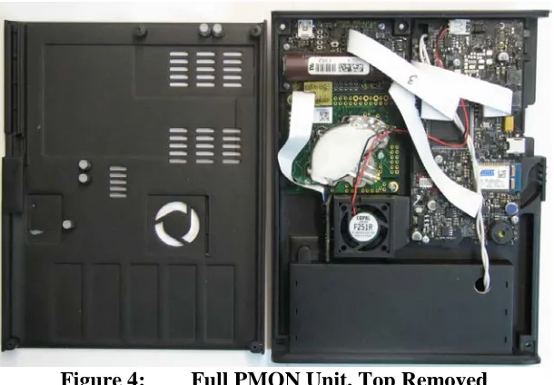
2.1 Previous Research
As part of previous research, a portable particle counter had been developed for the mobile PMON platform (Figure 4). The PMON was developed by the HSIL for the Federal Aviation Administration (FAA) and was intended to evaluate air quality and detect contaminants within airliner cabins. A complete PMON is composed of the motherboard, the OPC, a feedback controlled fan, and various sensors.
2.1.1 PMON Motherboard
The PMON’s motherboard is designed with flexibility in mind regarding sensor integration, data management, and portability. It currently serves as a critical element in the OPC, fully enclosing the topside of the channel. It comes equipped with Atmel’s AT32UC3A2 processor, which provides the control signals and analog-to-digital (ADC) channels required to operate all sensors and the OPC.
Flat-flex cable (FFC) headers offer connection points for daughterboards designed independently from the motherboard. These headers expand on the motherboard’s
original functionality through communication protocols such as Inter-Integrated Circuit (I2C), Serial Peripheral Interface (SPI), Universal Synchronous Asynchronous Receiver Transmitter (USART), and general purpose input output (GPIO). This makes the platform flexible and versatile, allowing sensors to be swapped whenever necessary. Besides communication protocols, direct current (DC) power is also provided to each sensor through its respective FFC connection point. Several daughterboards are already available from previous research and provided access to pressure, temperature, CO, and CO2 sensors for the PMON platform. Of these sensors, only temperature is required to aid the anemometer in calculating the airflow velocity. The daughterboard containing the thermistor was also used to fully enclose the flow channel. This allowed the thermistor to be placed within the flow channel. The thermistor board is the only preexisting
daughterboard used in this research.
storage can be used for storing sensor measurements as well as system log files for potential run-time issues. An initialization file containing options, settings, and
calibration information is also kept on the SD card. This allows certain system or sensor functionalities to be enabled or modified without the need for reprogramming. A mini Universal Serial Bus (USB) port could be used to access the SD card for added convenience.
Wireless communication, being fundamental for portability, is primarily
accomplished through Zigbit protocols. This allows each PMON unit to operate as part of a mesh network, effectively extending the communication range between the data sources and delivery points. By changing options in the SD card initialization file, a PMON unit could be designated as either a coordinator node or a sensor node. Coordinator nodes act as end points to the data flow in the mesh network and usually interface with a database either via local area network (LAN) or Wi-Fi. The sensor nodes in the mesh network simply pass along information from one unit to the next until received by a coordinator. Bluetooth is also available on some units, and a real-time data feed can be accessed on Bluetooth-ready devices such as a smartphone or tablet. An Android application was also designed by HSIL for real-time plot generations on these devices.
two pin header is available on the underside of the motherboard so that a coin cell battery could assist in maintaining the proper date and time for unpowered PMON units.
2.1.2 Airflow Channel
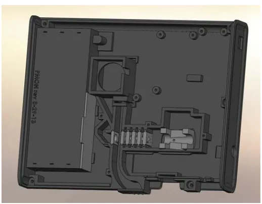
The airflow channel is a vital component to the particle counter system and is designed to provide laminar airflow orthogonal to a laser beam. The PMON’s channel is 10 mm deep by 6 mm wide and is approximately 50 mm long. The flow channel and the PMON’s enclosure are designed as a single component and cannot be separated (Figure 5).
Figure 5: PMON OPC Flow Channel and Enclosure
10,000 RPM, which is slightly under the fan’s maximum performance capability. After processing the error of the EMF pulse timing, the microcontroller updates the pulse-width modulation (PWM) signal used to control the fan voltage.
Figure 6: Fan Control Block Diagram
ANSYS computation fluid dynamics software was used to predict the behavior of the air through the channel. While the airflow velocity is largely dependent on the
rotational speed of the fan, all simulations were performed with an airflow velocity of 4 m/s and showed stable laminar flow. SolidWorks enabled the 3D CAD design of the channel, which could then be printed using stereolithography (SLA) technology.
Figure 7 demonstrates the airflow path relative to the incident laser beam. Air, signified as blue arrows, is pulled through the inlet and is then drawn through a curved path. The curved path is used to prevent external turbulences from having direct access to the flow passing under the photodiode. The red line represents the laser beam as it passes through the light blocks and crosses the flow channel. The point of intersection between the blue arrow and red length is the location of the photodiode.
Figure 7: PMON OPC Airflow Channel Showing Direction of Flow (Blue) and Incident Laser Beam (Red)
the channel inlet and outlet locations only. To prevent light from reflecting into the flow channel, both the motherboard and the flow channel have matte black finishes.
2. 1. 3 Firmware and Software
The PMON’s motherboard is set to run on a flexible codebase designed to easily select, enable, disable, and add sensors. Both low level and high level code is made to be modular, allowing quick changes between different platforms and setups. Each platform consists of a set of sensors appropriate for the intended research. A custom data manager routes the data flow going from each sensor source to the data log and wireless network.
While a database is made available, the data is more often viewed in real-time through a program called Sensor Monitor Lite, developed by HSIL. Sensor Monitor Lite allows the user to view all unit and sensor data from a designated serial port,
Transmission Control Protocol/Internet Protocol (TCP/IP) address, or data log file. Previously acquired data can also be obtained from a database and then viewed in Sensor Monitor Lite. The graphing window allows for dynamic panning and zooming of
captured data from one or more units. As an added feature, the data can be exported to a comma separated value (CSV) formatted file.
2.2 Existing Technology
2.2.1 Optical Particle Counters
Hall surmises that airborne particulate detection has been performed since people could see smoke from a fire [6]. Still, most particulate, especially that of PM2.5, is
invisible to the naked eye. Consequently, various particulate sensing technologies have been developed over time. These technologies vary considerably in design and
A device used in a study by the EPA consists of a technique that accumulates PM of various sizes on filters. At the end of a specified interval, each filter was removed and weighed to determine PM concentration levels. Impactors, cyclone heads, or specific filters could be used in order to capture particle sizes of interest [9]. While the device was capable of widespread use in many environments, its process required time for particle accumulation during which it could not be moved. Additionally, precise mass
measurements had to be taken after a specified duration of exposure to the particulate. As a result, this device is not capable of obtaining real-time measurements nor can it be considered portable [10].
The tapered element oscillating microbalance (TEOM) is another approach that also uses the mass of the particulate to determine ambient concentrations. Instead of accumulating the PM on a filter, the TEOM collects PM on a glass element that oscillates due to an electric field. As more PM is caught on the element, the overall mass increases, thus changing the oscillation frequency. This allows for data to be collected in real-time. Still, the TEOM makes no improvements in the realm of portability as the device requires a considerable amount of setup time and cannot be moved during operation [10].
In an effort to increase portability, optical particle counting techniques have undergone much exploration. One of the earliest optical methods involved a
voltage generated at the extinction diode. The size and number of voltage dips can be used to determine particulate size and concentrations, respectively.
However, detecting the absence of light is much more difficult than detecting light itself due to diffuse reflectance. As a result, a light scattering approach is capable of higher sensitivities [12]. In a light scattering OPC, the photodiode is placed at an angle away from the incident laser. As particulate traverses through the laser beam, light is scattered in many different directions. The photodiode then captures some of the scattered light and generates voltage pulses. The pulse amplitude and duration is then used to determine the particle’s size. The number of counts is scaled to determine the concentration in the ambient fluid. In comparison to the light obscuration method, the light scattering approach tends to be more costly due to the requirement of more sophisticated circuitry [11].
Some OPC designs combine both the scattering and obscuring techniques in order to cover a broader range of particulate sizes. For example, data from the laser extinction diode can be used to detect particulate sized 2.0µm or greater whereas the scattering diode can be used to count particles of finer sizes [11]. This approach greatly increases the complexity of the classification system in firmware as well as the required circuitry.
While extending the sensitivity range of OPCs, CPCs require additional apparatuses that make portability very difficult.
Of these optical methods, the single sensor scattering approach has been shown to be effective in producing smaller, less expensive particle counters. Dylos Corporation produces and sells single units for approximately $300 [14]. These units use a fan to drive the air through a flow channel. All data is collected through an attached screen or through a computer serial interface port (Figure 8). However, they do not contain any form of battery support and must remain connected to a power socket. They are also too large to be worn, being approximately 8 cm by 11 cm by 18 cm. As a result, these units are not portable. There is no particle size differentiation.
Figure 8: Dylos DC1100 Air Quality Monitor [14]
significantly higher. Depending on the desired model, each unit costs around $2000 to $4000.
2.2.2 Hot-Wire Anemometers
Hot-wire anemometers have arguably been in development since Boussinesq performed his studies on convective heat transfer with heated wires in 1905. A year later, King furthered Boussinesq’s research and made pivotal progress by experimentally verifying heat transfer results from potential flow around a cylinder. From there, the first measurements of subsonic flows were obtained by Dryden and Kuethe in 1929 using what is now known as a constant current anemometer. Since then, various circuit types have been used to both heat the wire and keep one characteristic variable constant: current, voltage, or temperature [15, 16].
The simplest anemometer is the CCA, being the first created [16]. The CTA followed a few years after the CCA in design [15] and advanced its sensitivity and efficiency. The latest hot-wire anemometer type is the CVA, originally patented by Sarma in 1993 [17].
In addition to the measurement of airflow velocities, other uses for the hot-wire anemometer have been found and studied. In one instance, the anemometer was used as a particle velocity detector in standing sound waves [23]. Gas concentration measuring with an anemometer was shown to be viable for certain types of gases during mixing [24]. A hot-wire anemometer was also shown to be capable of capturing particulate counts in [25].
Using hot-wire anemometers in real-time control problems has already been shown to be viable by Huang in [18]. Placing micro-machined anemometers and control surfaces at the lip of a jet, a closed loop feedback control system could be used to assist in eliminating jet engine screech. However, the anemometers used were
microelectromechanical systems (MEMS) and extremely small. MEMS-based
CHAPTER 3: OPTICAL PARTICLE COUNTER
This chapter discusses the approach used for particle counting in this research. OPC design and calibration methods are presented. The impact of external airflow disturbances is briefly discussed. A detailed explanation on the effects of these disturbances can be found in Chapter 6.
3. 1 Overview of Optical Particle Counting
The OPC used for this research was designed by the HSIL at Boise State University. Based on the prices of commercially produced OPCs, particle counting has been fairly limited to high-end research or large-scale industrial applications. In order to consider the custom OPC to be successful, it was required to match the performance of these commercial devices. This proved to be a difficult task, as the commercial devices were not always in agreement amongst themselves due to their differing approaches in design and calibration [6].
3.1.1 OPC Design
Three variations of the OPC had been developed in the HSIL, although only one was used in the PMON system. The first OPC consisted of a single photodiode placed above the laser’s incident area in the flow channel. The other two designs each contained a second photodiode, one placed in tandem and the other placed orthogonal to the
Particles detected at the photodiode produces a very small current. A
transimpedance amplifier is used to convert the photodiodes output current to a voltage. Two additional amplifiers are then used to scale the resulting voltage. The first amplifier provides a large amount of gain to facilitate the capture of weaker pulses caused by very small particles. The second amplifier’s gain is set much lower so that larger particles would not saturate the ADC input and can be classified appropriately. While the actual size of each particle is difficult to determine in this setup, calibration methods can be employed to adjust the threshold between the small particle and large particle counts. By default, the small particle detection range is set between 0.3 µm and 1 µm. Anything larger than 1 µm was considered a large particle with a maximum detection limit of 25 µm.
3.1.2 OPC Calibration
Calibration remains a vital step in the development of each OPC. The accuracy of every particle counter is highly dependent on the reliability and consistency of the
Each PMON unit undergoing calibration was placed into a chamber along with the Aerotrak handheld OPC. Pressurized air could then be fed into this chamber via one of four paths. The diagram in Figure 9 demonstrates the layout for this system and is also described in further detail in [6]. The first path was the flush line, which was a direct path from the source to the chamber. The air source was relatively clean and was capable of reaching concentration levels less than 1000 particles per liter (PPL). The next three paths all stemmed from the system feed route, which ran in parallel to the flush line. A collision nebulizer was placed in between all three routes and the system feed.
The first path coming from the nebulizer fed directly into the chamber, allowing cold particulate to remain intact. The second path ran through a heated pipe before allowing the particulate to enter the chamber. The last path contained desiccant to dry the particulate flowing into the chamber.
The cold and hot paths were used for greater particulate counts and required the nebulizer to be filled with a combination of tap water and de-ionized (DI) water. The impurities of the tap water were more than enough to generate counts in the millions per cubic foot. The DI water was used to dilute the tap in order to keep the generated
Figure 9: Particle Generation System and Chamber Used for OPC Calibration [6]
The desiccant path provided a means of generating particulate of specific sizes and could also extend the obtainable particulate sizes. It did not require any tap water and instead used a mixture of polystyrene latex (PSL) and DI water in the collision nebulizer. The PSL, specifically designed for particle counter calibrations, was generally kept at sizes close to the threshold used to distinguish small and large counts: 0.6μm, 0.8μm, and 1.0μm.
outfitted with a small laser module. These, being low cost laser modules, varied in beam shape and intensity. Each laser had to be characterized prior to calibration to ensure that it was capable of obtaining minimum levels of power output and that its shape would not drastically alter the ambient light levels in the airflow channel.
Another important factor was the airflow velocity through each unit’s channel. Despite the simulations performed in ANSYS, the actual airflow velocity was never experimentally investigated in [6]. Hypothetically, a higher airflow velocity could potentially increase the number of particles flowing through the beam, leading to higher counts. At the same time, the increased velocity would also decrease the amount of time the particle spent in the laser beam. Both the higher counts and pulse changes could drastically alter the particulate measurements. Therefore, it was important to ensure each fan operated at the same RPM. Unfortunately, even if each fan was run at maximum power, discrepancies in the range of 1000 RPM would appear. This was a problem even for fans of the same model and manufacturer.
The original solution devised was to place a feedback control loop into the fan’s power line [6]. Using the back EMF from the fan’s magnetic pole pairs, each rotation of the fan could be tracked. The firmware for the particle counter would then count the number of rotations over a certain interval of time in order to determine the actual RPM. The feedback control loop could then use PWM to change the amount of voltage applied to the fan until a balance was found.
concentration measurements may have been greatly affected. This idea was first explored by placing a 12 V fan with a static RPM orthogonal to the OPC intakes.
Figure 10: External Airflow Disturbance Test in OPC Calibration Chamber
Figure 11: External Airflow Disturbance Test Results
While it was originally expected that the PPL measurement of Unit B might increase due to more particles traveling through the laser beam, the assisted airflow actually resulted in a large decrease of its PPL measurements. This was potentially caused by a decrease of the pulse width or amplitude generated by each particle. Changing pulse characteristics could lead to missed trigger conditions or inaccurate particle classifications.
In order to understand what may be required to properly compensate for
measurement inaccuracies, the effects that varying airflows have on the particle counter’s hardware will need to be explored. This is discussed further in Section 6.1.2, Effects of Varying Airflow on Particle Counts.
0.00E+00 5.00E+00 1.00E+01 1.50E+01 2.00E+01 2.50E+01 3.00E+01 3.50E+01 4.00E+01
29 34 39 44 49 54
PPL
(
1
0
3)
Time (Seconds)
Unit A
CHAPTER 4: HOT-WIRE ANEMOMETER
The contents of this chapter are centered on the physical equations used by the hot-wire anemometer. By exploring the relationships between convective heat transfer, fluid dynamics, and resistance equations, expected behavior of the anemometer can be predicted.
4.1 Theory
Convective heat transfer plays a direct role in the calculation of fluid velocities. This is accomplished by heating a thin wire to a known temperature and then passing a fluid of a known temperature around the wire. The change in the wire’s temperature is indicative of the fluid’s velocity. Physical equations are required to determine the temperature of the wire and the heat transfer coefficient used in the end calculation [15, 16, 24].
The first equation is that of the relationship between the wire’s resistance and its temperature,
𝑅𝑤 =𝑅0[1 +𝛼(𝑇𝑤− 𝑇0)]. (1)
where 𝑅𝑤 is the new resistance of the wire, 𝑅0 is the resistance at the time of calibration,
𝑇𝑤 is the current temperature of the wire, 𝑇0 is the temperature of the wire at time of
selected for this research. Tungsten’s temperature coefficient is 4. 5 × 10⁻³ (𝐶°)−1. Since the present resistance of the wire is more easily found than the temperature of the wire, Equation (1) is rearranged for𝑇𝑤, or
𝑇𝑤 = 1𝛼 �𝑅𝑅𝑤
0 −1�+𝑇0. (2)
At this point, both the resistance of the wire and the temperature of the wire should be known. If either the current through the wire or the voltage across the wire is also known, then the power into the wire can be determined. The power dissipated at the wire is used to increase its temperature, which is then affected by several types of heat transfer: radiation, conduction, and convection. If the majority of the heat transfer is performed through convection, then both radiation and conduction can be assumed to be negligible, leading to Equation (3),
𝑃𝑤 =ℎ𝐴𝑤�𝑇𝑤− 𝑇𝑓�. (3)
where 𝑃𝑤 is the power dissipated at the wire, ℎ is the heat transfer coefficient, 𝐴𝑤 is the cross section area of the wire, and 𝑇𝑓 is the temperature of the fluid. This follows the assumption that all power dissipated at the wire is accomplished through convection. Unfortunately, this assumption may not always be accurate. If the temperature of the wire exceeds a certain level, radiation heat transfer will begin to dominate the net energy loss in the system. The end result is a decrease in convective sensitivity and wasted power.
The heat transfer coefficient is a function of the airflow velocity; it provides the necessary connection between the airflow physical equations and circuit equations. This is accomplished through the Nusselt number. The Nusselt number (𝑁𝑢) is a
on the geometry of the surface, it is always dependent on the Reynolds number (𝑅𝑒), and the Prandtl number (𝑃𝑟). For a wire, Kramers experimentally demonstrated [30] that
𝑁𝑢 =𝐴𝑃𝑟𝑝+𝐵𝑃𝑟𝑞𝑅𝑒𝑛, (4)
where 𝐴,𝐵,𝑞,𝑝, and 𝑛 are constants discovered at time of calibration. The Reynolds number, a ratio between inertial and viscous forces, is defined as
𝑅𝑒= 𝑈𝑑𝜈𝑤. (5)
In Equation (5), the Reynolds number is composed of the fluid velocity𝑈, wire diameter𝑑𝑤, and the kinematic viscosity𝜈. The Prandtl number, a ratio between viscous and thermal diffusion rates, is based on the temperature and type of fluid, which, in this case, is air. The identity for the Nusselt number offers the final connection point between all the expressions:
𝑁𝑢 = ℎ𝑑𝑤
𝑘 . (6)
In Equation (6), ℎ is the heat transfer coefficient, 𝑑𝑤 is the diameter of the wire, and 𝑘 is the thermal conductivity of the fluid. Substituting Equations (5) and (6) into Equation (4) yields
ℎ𝑑𝑤
𝑘 𝑁𝑢 =𝐴𝑃𝑟𝑝+𝐵𝑃𝑟𝑞�
𝑈𝑑𝑤
𝜈 �
𝑛
. (7)
Since 𝑑𝑤 and 𝑘 are both constants, they can be rearranged on the other side of the equation and absorbed by 𝐴 and𝐵, leaving
ℎ =𝐴𝑃𝑟𝑝+𝐵𝑃𝑟𝑞�𝑈
𝜈�
𝑛
. (8)
temperature may be varied and will be measured by a thermistor for proper
compensation. Rearranging Equation (3) and substituting into Equation (8) reveals that
𝑃𝑤
𝐴𝑤�𝑇𝑤 − 𝑇𝑓�=𝐴𝑃𝑟
𝑝+𝐵𝑃𝑟𝑞�𝑈
𝜈�
𝑛
. (9)
Finally, Equation (9) can be modified to come to the final expression for fluid velocity: 𝑈= � 𝐷𝑤𝑃 𝑘𝐴𝑤𝐵𝑃𝑟𝑞�𝐷𝜈 �𝑤 𝑛 �𝑇𝑤 − 𝑇𝑓� − 𝐴𝑃𝑟𝑝 𝐵𝑃𝑟𝑞�𝐷𝑤 𝜈 � 𝑛� 1 𝑛 . (10)
As can be seen in Equation (10), calculating the airflow velocity can become fairly computationally intensive, especially for a processor that has to deal with other tasks. This equation will need to be simplified to make it viable for a microcontroller. Further discussion on the simplification, approximation, and application techniques of this equation can be found in Section 6.2.4, Anemometer Calibration.
4.2 Constant Current Anemometer (CCA)
Figure 12: CCA Circuit [15]
The CCA’s simplicity is its strongest advantage. Component costs are generally lower than those required for the CTA and CVA. Computing results from a CCA is straightforward, requiring little processor time. Operating regions can be easily selected by choosing different resistor values for the bridge, and no stability problems will occur since the system remains open loop. Unfortunately, the constant current leads to a lack of sensitivity, especially at high frequency velocity changes. This is due to the continuous heating of the wire. Extended heating periods without airflow will result in temperatures higher than what is desirable. Radiation and conductive heat transfers will prevent the wire’s temperature from increasing indefinitely, but will also lead to wasted power.
4.3 Constant Temperature Anemometer (CTA)
Instead of using a constant current supply, the CTA (Figure 13) contains a
variable current supply that is controlled by an analog feedback loop. Just as in the CCA, a Wheatstone bridge is used to apply a voltage across the wire and to produce a reference voltage. The error between the wire voltage and the reference voltage is then amplified and used to increase or decrease the current delivered from the supply. The current is also captured as airflow velocity data.
Figure 13: CTA Circuit [15]
The result is that the temperature and resistance of the wire is maintained whether or not fluid fluctuations exist. This leads to the obvious advantage that no power is wasted overheating the wire. A second advantage is that the temperature of the wire does not change. Ideally, the amount of current being drawn should be almost identical in every instance where the airflow velocity is the same. In other words, the time constant for heating the wire is removed from operation once the wire has been initially heated. This allows the CTA to operate at frequencies much higher than that of the CCA.
Some methods have been employed to counteract this disadvantage, such as adding a second feedback loop capable of altering the parameters of the initial feedback loop as described by Ligęza in [31]. Another disadvantage is that the CTA’s response is limited by the amplifier’s response time in increasing the current flow. Airflow fluctuations that occur at a frequency outside the operation amplifier’s functional bandwidth cannot be properly compensated and will not appear in the data acquired. Probe lead length also places a role in the performance of the anemometer. Long leads are susceptible to radio frequency (RF) noise, which can also be a problem inherent to the CCA. This RF noise can be a significant problem if large gains are applied to make up for small temperature differences between the wire’s operating temperature and the ambient temperature. The system is closed loop and can fall into instability if the Wheatstone bridge is not properly balanced.
4.4 Constant Voltage Anemometer (CVA)
The CVA (Figure 14) accomplishes its constant voltage by placing the wire in a T-resistor network of an amplifier’s feedback loop, removing the bridge that was seen in the CCA and CTA. Even if the wire’s resistance changes, the voltage remains constant, thus allowing the current through it to be read as airflow velocity data.
With the return of the time constant to the system’s operation, bandwidth issues can be a problem for higher frequencies. The CVA’s bandwidth is immediately greater than the CCA’s bandwidth, but should be improved by certain techniques such as placing a resistor-capacitor (RC) network in the feedback loop of the amplifier. An additional composite amplifier can be placed on the output of the primary amplifier to further enhance the bandwidth [17]. While probe lead lengths do not contain capacitance problems, they do contain resistances that have been shown to increase thermal lag, decreasing accuracy. The lead resistance should be measured prior to operation in order to predict the effects of the additional thermal lag [32].
CHAPTER 5: HARDWARE DESIGN
This chapter presents the design and hardware implementation of CCA, CTA, and the anemometer probe. The components were selected based on results of simulations. Analysis of each implementation is also shown in this chapter.
5.1 Anemometer Probe
As described in Section 1.2, the anemometer probe is the sensing point of a hot-wire anemometer. It is composed of the hot-wire and a supporting structure. The structure is used to hold the wire taut and to direct the airflow around the wire. It also provides an interface between the wire and the leads connected to the heating circuit.
5.1.1 Wire Resistance Estimation
The starting resistance of the wire is affected by its material type and geometry, as described by
𝑅𝑤 = 𝜌𝐿𝐴 𝑤
𝑥𝑤, (11)
the leads into the probe will contain resistance, the actual starting value for𝑅𝑤 is estimated to be slightly higher.
The maximum value of 𝑅𝑤 was dependent on the type of anemometer and its circuit’s bridge resistor values. If the ratio between balanced legs was 1: 10, then the top resistance of the probe leg needs to be 10% of the value of the top resistor of the
reference leg. As the resistance of the wire increased, the wire voltage increased, which caused the bridge difference to go to zero. If the voltage across the wire surpassed the voltage across the lower resistor on the reference leg, then the output of the bridge would become negative. Negative voltages require more power regulation and signals to manage making data acquisition unnecessarily difficult. Therefore, they were avoided by making the lower resistor of the reference leg a value high enough to prevent this from occurring.
The balancing of the bridge legs leads to the implication that the bottom reference resistor can be used to control the operating temperatures for both the CCA and CTA. For example, if the resistance of the probe was 3. 3Ω, then the lower reference resistor could be 36Ω. Using Equation (2), Figure 15 was generated. With the assumption that
Figure 15: Estimation of Temperature for Resistances of Tungsten Wire
5.1.2 Probe Design and Implementation
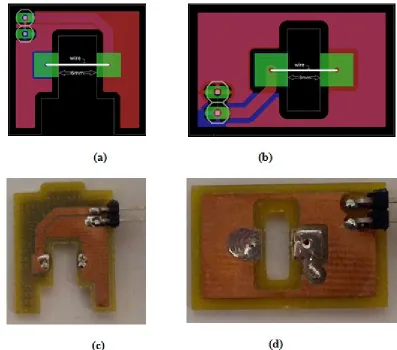
Two probe types, one for the existing OPC flow channel (Figure 16a) and another for the test channel (Figure 16b), were created. The length of each probe wire was
dictated by the width of each flow channel. Since the test channel’s width was 3 mm, the effective length of the wire was also 3 mm. Following the same convention, the probe wire for the OPC had an effective length of 6 mm. The differing wire lengths between each channel type led to differing resistances for each probe. The thickness of the white wires in Figure 16 has been exaggerated for clarity.
280 300 320 340 360 380 400
3.0 3.5 4.0 4.5 5.0
W
ir
e T
em
p
er
at
u
re
(K
)
Figure 16: (a) Probe Layout for the OPC Flow Channel, (b) Probe Layout for the Test Channel, (c) Actual OPC Probe, (d) Actual Test Probe
Both probes were two layer PCBs with copper pads containing 0.6 mm holes positioned on opposite sides of a rectangular cutout. Unlike the test channel’s probe, the OPC’s probe had a cutout that was not fully enclosed since the prototype enclosure dimensions would not permit a groove extending into the floor of the channel. The size of the probe was made to be only as large as structural stability required. A two-pin right angled header extended off the side, each pin giving access to one end of the wire.
wire was effectively controlled by the locations of electrical contact, each probe needed to have its wire soldered in the exact same locations. Ideally, this location is as close to the cutout as possible such that the length of the wire is close to the actual width of the flow channel. Excess solder was consciously avoided as it made inserting the probe into the channel a much more difficult task.
Applying extreme amounts of heat to the wire may have resulted in damages. However, ensuring that the flow channel was fully enclosed around the wire required specifically shaped material that could be reproduced consistently. PCB proved to be the best solution at hand given the resources available.
Both PCBs were designed with a cutout approximately the same width as that of their respective flow channels. The test channel’s cutout extended into the floor of the flow channel and the OPC’s channel contained grooves on the sides. The test channel was designed to simply provide laminar flow for calibration purposes. No photodiode or laser was present in the system and the anemometer could be placed anywhere within the laminar region. The placement of the anemometer into the OPC channel, however, required laminar flow at a location downwind from the photodiode. This was required due to the possibility that the anemometer’s wire could potentially disrupt the laminar flow if resonated at specific frequencies. Any turbulence in the channel could cause the OPC to misread particulate data.
used in order to simulate proper behavior when running in the PMON platform. The leads’ combined resistance was approximately 0.145 Ω.
5.1.3 Results
After the assembly of a probe, its resistance was measured to ensure proper connections were made between the wire and the solder joints. If the results varied too often or an open circuit was found, the joints were re-soldered and new wire was applied. It was commonly found that each smaller probe was around 2.4 Ω and each larger probe was around 3. 5Ω, as predicted in Section 5.1.1. While not entirely certain, the excess resistance may have been a result of wire damage that may have occurred during the soldering process. Applying excessive heats to the solder pad may have exposed the wire to unnecessary temperatures for prolonged periods, causing the wire to expand. Cooling the wire would cause it to contract and possible form breakages along its exterior. As a precaution, the lowest soldering temperature available was applied to the pads.
The connection points for each wire end were placed as close to the edge of their respective pads as possible. This assisted in achieving consistent wire lengths. Any connections made further from the edge also resulted in an instant increase of the wire’s starting resistance. Ultimately, it took several creation iterations before usable probes were produced.
5.2 Constant Current Anemometer
Due to its ease of implementation, a CCA was the first proof of concept prototype. The design of each hot-wire anemometer type began with LTSpice
was not necessary to include a large bandwidth in each circuit design. These prototypes provided a platform around which the rest of the firmware could be developed.
5.2.1 CCA Simulation
Using LTSpice, the CCA circuit was simulated to determine operating
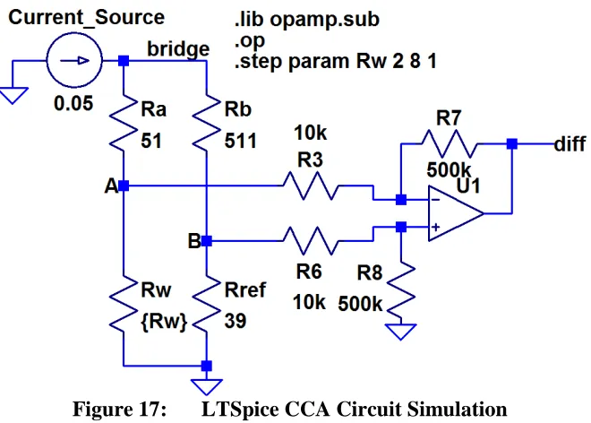
boundaries. A constant current source delivered 50 mA to the bridge, overheating the wire and generating the reference voltage. The top resistors of the bridge, 𝑅𝑎 and𝑅𝑏, were held to a proportion of 1:10, respectively (Figure 17). This meant that the bridge would balance when 𝑅𝑤 achieved a value equivalent to a tenth of the resistance of𝑅𝑟𝑒𝑓. Since the value of 𝑅𝑤 was dependent on the type of probe being used, two primary operating points for 𝑅𝑟𝑒𝑓 were tested.
Figure 17: LTSpice CCA Circuit Simulation
resistance was at its lowest point. As the motherboard does not supply negative voltage, the differential amplifier could only output zero volts. This occurred when the value of
𝑅𝑤 exceeded a tenth of the value of𝑅𝑟𝑒𝑓. While 80 mV was easily within the input range
of the ADC, it did not make good use of the ADC’s 12-bit resolution. The differential amplifier stage was altered to provide a gain of 50 to the difference of the voltages. Applying this gain resulted in an output voltage range of 4V to 0V. While this placed the operation slightly outside the acceptable range of the ADC, the average minimum
resistance of the 3 mm probe was 2.5Ω. Figure 18 shows that the voltage output for a 2.5Ω wire was 3V, which was within the ideal operating range.
Figure 18: LTSpice CCA Simulation Voltage Output over Wire Resistance
Applying a similar approach for the probe with the 6 mm wire, 𝑅𝑤 was stepped from 3 to 5Ω in increments of 0.1Ω. This time, a 47Ω resistor was set in place for𝑅𝑟𝑒𝑓. Similar to the results seen for the 3 mm probe simulation, the voltage output of the circuit varied from 3.6 to 0 V, being slightly over the operating range of the ADC. Once again, this was ignored due to the actual resistance of the probes being higher than 3Ω.
0 0.5 1 1.5 2 2.5 3 3.5 4 4.5
2 2.5 3 3.5 4
V o lta g e O ut p ut ( V )
5.2.2 CCA Design
The anemometer circuit was placed on a two-layer PCB with a current source, Wheatstone bridge, differential amplifier, and an ADC. On the same board was also a thermistor circuit, which was used to detect the ambient temperature for the velocity calculations. All integrated circuits operated at 3. 3 𝑉 with the exception of the current source, which was powered at 5 𝑉.
The constant current source aimed to provide approximately 50 mA to the bridge in order to generate the reference voltage and to heat the filament. By using a MAX1818 linear voltage regulator and placing a resistance between its output and ground (see Figure 19), a constant current could be generated for any load between the regulator’s ground and the circuit’s actual ground.
Figure 19: CCA Eagle Schematic
The two voltage levels were then sent to a differential amplifier with the probe voltage fed into the negative input. The operational amplifier was powered by a 3.3V supply on its positive rail and grounded on its negative rail to prevent negative values from being propagated. After a gain of 50 was applied to the signal by the amplifier, the output could be read by a digital multi-meter (DMM) probe or through an ADC. For this project, ST Microelectronics’ TS9222 was selected for the operational amplifier and Texas Instruments’ ADC121C021 was used for the analog-to-digital conversion. The extra unused amplifier in the package was set as a voltage divided source follower to prevent errant behaviors or added noise.
5.2.3 CCA Results
The CCA was tested using the test airflow channel with a probe resistance of 3.46Ω. Using an airflow velocity range between 0 and 3.1 m/s, the reported ADC voltages varied between 2.87 and 3.16 V (Figure 20). Placing the probe in a sleeve lacking airflow revealed a noise floor of approximately 1 to 2 mV. This offered a great SNR for airflow velocities below 3 m/s. However, as the speed of the air increased beyond that point, the resulting voltage change diminished, causing the noise to become more dominant.
Figure 20: CCA Output Voltage as a Function of Airflow Velocity
An additional problem also occurred during prolonged periods of time where the probe experienced no airflow. The steady-state temperature of the wire was often
dependent on external factors, causing the behavior of the anemometer to lack
consistency. While this issue is potentially solvable in firmware, the end result would be a reduction in accuracy. These problems, coupled with the power inefficiencies,
encouraged the development of a CTA. 2.850 2.900 2.950 3.000 3.050 3.100 3.150 3.200
0.00 1.00 2.00 3.00 4.00
F eed b ack V o lt ag e (V )
5.3 Constant Temperature Anemometer
A constant current caused overheating, which resulted in inaccuracies and wasted power. A CTA version of the device was developed to solve the accuracy and power problems of CCA.
5.3.1 CTA Simulation
The CTA circuit was first simulated in LTSpice to determine the range of stable behavior across multiple probe resistances and DAC voltage inputs (Figure 21). The reference leg of the bridge acted as a voltage divider on the output voltage of the DAC. Setting 𝑅𝑏 and 𝑅𝑐 equal to each other cut the DAC output voltage in half, allowing it slightly higher resolution control. Since the voltage generated at the reference leg was designed to be higher than the wire voltage, it was fed into the positive input of the amplifier. A gain of 10 is applied to the voltage difference. If the DAC voltage is held at a constant 1V and the probe resistance is stepped from 3Ω to 8Ω, the expected current through the wire is found to be approximately 69 mA to 36 mA, respectively.
The expected feedback voltages hit a maximum value of 2.87V when the resistance is at its minimum. It is important to note that while the DAC voltage is held constant in the simulation, it will vary based on the resistance of the wire to ensure proper temperature compensation. Since the current through the wire decreases as its resistance increases, the rate at which it overheats is diminished. This is necessary to ensure a constant temperature is obtained during normal operation. However, if the starting
resistance of the wire is higher than its original calibration value, its overheat rate will not match its previous levels, causing lower sensitivities and inaccuracies.
5.3.2 CTA Design
The circuit was designed using CadSoft’s EAGLE PCB design software and printed on a two-layer copper board. The board’s dimensions were 30.55 mm by 13.3 mm and contained all components on a single side for ease of placement within the PMON enclosure. A Flat Flex Cable (FFC) was used to extend power and protocol signals from the motherboard to the CTA daughterboard. Due to the number of sensors contained within a PMON unit, the I2C protocol remained the viable option for adding additional sensors. This same I2C port was also used for two other daughterboards; therefore, the anemometer daughterboard provided yet another FFC header to carry out the supply and control signals. A right-angled 2-pin header acted as the probe’s
connection point. The anemometer connected to the probe either via short wires or directly, depending on the desired placement location of the board within the PMON enclosure.
The CTA makes use of a digital-to-analog converter (DAC) for calibration
not connected to the feedback voltage. This moves more of the CTA operation into firmware, allowing for greater flexibility.
The components were selected based on simulated operating ranges, such as the wire current and feedback voltage. The MCP4728 from Microchip Technology was selected as the DAC for its 12-bit resolution and I2C interface. Sourcing current to the wire required the use of a specialized amplifier. STMicroelectronics’ TS9222 is a rail-to-rail high output operational amplifier capable of providing up to 80 mA to a load, which is more current than required according to the simulation. The ADC used in the design was Texas Instrument’s ADC121C021. Similar to the DAC, this ADC was also 12 bits in resolution and was I2C compatible.
The CTA EAGLE schematic, shown in Figure 22, implements the simulated circuit as shown in Figure 21. One minor difference between the simulation and the implementation is that the reference leg contains 10kΩ resistors instead of 3.3kΩ. This did not make any difference to the operation of the anemometer as the voltage division ratio remained the same.
5.3.3 CTA Results
The CTA circuit was capable of obtaining the desired operating levels without saturating the ADC. However, stability of the circuit began to fade as the probe resistance was increased to levels beyond 5Ω. Increasing the DAC output may be required to assist in stability for highly resistive probes. Probes with resistances exceeding DAC
compensation will need to be replaced.
Figure 23: CTA Feedback Voltage as a Function of Airflow Velocity
The feedback voltage for a given probe varied across a range suitable for
obtaining accurate airflow measurements. Using a 2.67Ω probe 3 mm in length, feedback voltage was plotted as a function of airflow velocity (Figure 23). A paper sleeve was placed over the probe to test no flow conditions. This showed that equilibrium between overheating and alternative heat transfers was accomplished at around 2.67V. When placed in the test channel, airflow velocity was varied by changing voltage to the fan. The results showed a non-linear relationship between the voltage and flow velocity, as
expected. The voltage appeared to asymptotically approach 2.74V as the speed was increased above 6 meters per second.
2.540 2.560 2.580 2.600 2.620 2.640 2.660 2.680
0 1 2 3 4
F eed b ack V o lta g e ( V )
Expectedly, the voltage feedback was not consistent for all starting resistance values for the different probes. A decline in the operating point appeared to drop logarithmically as the value of the resistance increased.
Figure 24: Operating Feedback Voltage at No Flow Conditions as a Function of Probe Starting Resistance
A lower operating point also indicates a lower operating temperature. Consequently, a higher probe resistance negatively impacts the airflow velocity
resolution of measurement. A higher DAC output can be applied to assist in off-setting the loss of sensitivity.
1.5 1.7 1.9 2.1 2.3 2.5 2.7 2.9
2 4 6 8 10
F
eed
b
ack
V
o
lta
g
e (
V
)
CHAPTER 6: FIRMWARE DESIGN
This chapter covers the implementation of the OPC and anemometer firmware. The effects of airflow velocity on particulate data characteristics are shown. Methods of measurement compensation and fan control are then discussed.
6.1 Optical Particle Counter Firmware
The OPC firmware was designed as part of previous research and the majority of the code remained unmodified during development of the CTA compensation method. The unchanged portions of the code are not thoroughly discussed in this research and can be found in [6]. The modified areas, including the original particle counting method and the proposed anemometer enhanced method, are discussed.
6.1.1 Original Counting Method
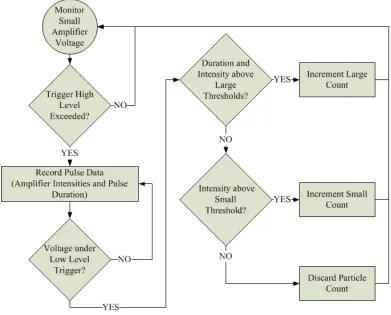
Figure 25: Simplified Particle Processing Algorithm Flowchart
Similar to the CTA, the OPC requires experimental data and a gold standard for proper calibration. Comparisons between the gold unit’s count numbers and the non-calibrated unit’s count numbers are performed using MATLAB scripts. The output of these scripts is a table of several values that can be set in the system configuration as calibration factors. Following Figure 25, a trigger value dictates when a pulse signifying a particle is large enough to begin the measurement process. Once the measurement process is complete, threshold values are then compared to the pulse intensity and duration in order to assign the count a bucket: small or large. Based on the counting interval, the buckets are periodically scaled by values to determine the ambient
Part of the calibration process for a PMON includes the addition of a sample scalar applied to a bucket prior to reporting the concentration results (Figure 26). This sample scalar primarily represents a means of scaling the volume of air sampled to another volume of the desired metric (e.g., liters). However, this sample scalar can also account for the difference of several possible variables between the gold standard and a unit undergoing calibration. For example, one PMON may contain a laser with a lower than normal output power. Consequently, really fine particles may produce pulse amplitudes smaller than what is determined to be noise. On the other hand, a unit could have a more powerful laser and produce higher pulse amplitudes. The calibration method would ensure that all units could agree on an ambient concentration level by adjusting the sample scalars and threshold values for each.
6.1.2 Effects of Varying Airflow on Particle Counts
Another physical variance that is compensated through the sample scalar is the airflow velocity. When the units were previously designed, they were assumed to operate with constant laminar flow through the channel. However, the volume of air being sampled, loosely expressed in cubic feet per minute (CFM), varies alongside the airflow velocity. In this instance, using a static sample scalar no longer provides accurate data.
If the particulate is assumed to be evenly distributed and the air that carries it incompressible, then a change in the airflow velocity should result in a proportional change of the numbers of particles traveling through the beam. This is reflected in the identity of volumetric flow rate where
𝑄 =𝑉𝑓𝐴. (12)
In Equation (12), 𝑄 represents the volumetric flow rate (e.g., CFM), 𝑉𝑓 is the velocity of the fluid, and 𝐴 is the cross-sectional area through which the air passes. Therefore, any deviation of the airflow velocity from what was used during OPC calibration should be reflected in the particle count linearly.
were then captured wirelessly as the power to the fans was lowered every several minutes.
Figure 27 shows the particulate concentration measurements of Unit A and Unit B during the experiment. The airflow velocity through Unit B was also plotted on the secondary axis for ease of comparison. At a glance, the relationship between airflow velocity and PM measurements does appear to be fairly linear for velocities under 5 m/s. The error between the units regarding PM concentration measurements is considerably large for airflow values much greater or less than 3 m/s. In one of the worst cases, when the airflow velocity was nearly 5 m/s, the difference was about 10,000 PPL. At that airflow velocity, for any given particle concentration inside the chamber, Unit B should produce approximately 140% the value that of Unit A. At the opposite end, where the airflow velocity drops below 1 m/s, the difference was also about 10,000 PPL, or 60% that of Unit A’s measurement.
Figure 27: Effects of Varying Airflow on Particulate Measurements -1 0 1 2 3 4 5 6 0 5 10 15 20 25 30 35 40 45
7000 8000 9000 10000 11000
Airflow Velocity (m/s) PPL (10
3)
Time (Seconds) Unit A Small PM
Unit B Small PM

![Figure 8: Dylos DC1100 Air Quality Monitor [14]](https://thumb-us.123doks.com/thumbv2/123dok_us/8921887.1842321/31.612.210.423.357.600/figure-dylos-dc-air-quality-monitor.webp)
![Figure 9: Particle Generation System and Chamber Used for OPC Calibration [6]](https://thumb-us.123doks.com/thumbv2/123dok_us/8921887.1842321/37.612.137.515.72.376/figure-particle-generation-chamber-used-opc-calibration.webp)