Modeling the probability distribution of positional errors incurred by residential address geocoding

Open Access

Research

Modeling the probability distribution of positional errors incurred

by residential address geocoding

Dale L Zimmerman*

_{, Xiangming Fang}

_{, Soumya Mazumdar}

_and

Gerard Rushton

Address: 1_{Department of Statistics and Actuarial Science and Department of Biostatistics and Center for Health Policy and Research, University of}

Iowa, Iowa City, IA 52242, USA, 2_{Department of Statistics and Actuarial Science, University of Iowa, Iowa City, IA 52242, USA and} 3_Department

of Geography, University of Iowa, Iowa City, IA 52242, USA

Email: Dale L Zimmerman* - [email protected]; Xiangming Fang - [email protected]; Soumya Mazumdar - [email protected]; Gerard Rushton - [email protected] * Corresponding author

Abstract

Background: The assignment of a point-level geocode to subjects' residences is an important data assimilation component of many geographic public health studies. Often, these assignments are made by a method known as automated geocoding, which attempts to match each subject's address to an address-ranged street segment georeferenced within a streetline database and then interpolate the position of the address along that segment. Unfortunately, this process results in positional errors. Our study sought to model the probability distribution of positional errors associated with automated geocoding and E911 geocoding.

Results: Positional errors were determined for 1423 rural addresses in Carroll County, Iowa as the vector difference between each 100%-matched automated geocode and its true location as determined by orthophoto and parcel information. Errors were also determined for 1449 60%-matched geocodes and 2354 E911 geocodes. Huge (> 15 km) outliers occurred among the 60%-matched geocoding errors; outliers occurred for the other two types of geocoding errors also but were much smaller. E911 geocoding was more accurate (median error length = 44 m) than 100%-matched automated geocoding (median error length = 168 m). The empirical distributions of positional errors associated with 100%-matched automated geocoding and E911 geocoding exhibited a distinctive Greek-cross shape and had many other interesting features that were not capable of being fitted adequately by a single bivariate normal or t distribution. However, mixtures of t distributions with two or three components fit the errors very well.

Conclusion: Mixtures of bivariate t distributions with few components appear to be flexible enough to fit many positional error datasets associated with geocoding, yet parsimonious enough to be feasible for nascent applications of measurement-error methodology to spatial epidemiology.

Published: 10 January 2007

International Journal of Health Geographics 2007, 6:1 doi:10.1186/1476-072X-6-1

Received: 17 November 2006 Accepted: 10 January 2007

This article is available from: http://www.ij-healthgeographics.com/content/6/1/1

© 2007 Zimmerman et al; licensee BioMed Central Ltd.

Background

It is becoming increasingly common in public health studies to use the spatial locations of study participants in statistical analyses, for example to test for geographic clus-tering of disease or to estimate relationships between environmental exposures and disease. Indeed, statistical methods for spatial epidemiology are developing rapidly, and the growing list of book-length treatments of the sub-ject include [1-4]. In order to utilize subsub-jects' locations in a spatial analysis, it is necessary, of course, to define and ascertain these locations. Historically, the spatial location of a person has been defined as the person's place of resi-dence; however, recognition of human mobility and the fact that many causative exposures occur outside the home have generated recent attempts to expand this defi-nition to daily activity spaces and such constructs as time geography and pathogenic paths; for a brief review see [5]. Nevertheless, place of residence currently remains the typ-ical representation of each subject's location in public health studies.

The spatial coordinates of a place of residence are usually not measured directly; rather, the residential address is given a location reference, known as a geocode. The geoc-ode may be defined as the latitude and longitude coordi-nates or a point in some other coordinate system, or as a statistical tabulation area such as a U.S. Census tract, block group, or block. Here, unless noted otherwise, we use the point rather than areal definition. Several distinct methods for geocoding exist, including visiting the resi-dence with global positioning system (GPS) receivers, identifying the residence on orthophoto maps based on aerial imagery, and matching the address to a digital street map. The latter can be done in batch mode for large num-bers of addresses and when done this way is often called "automated geocoding." Recently, a new method of auto-mated geocoding has been developed that matches an address to parcel descriptions of legal property bounda-ries developed by assessors, but this method has not yet been widely adopted. The U.S. Census Bureau is develop-ing such a parcel-level geocode for all U.S. addresses, but the public does not and will not have access to these geoc-odes. Accordingly, automated geocoding here will refer to the widely used practice of using a geographic informa-tion system (GIS) to match an address to a street name and address range in a digitized street reference map and then estimate, via interpolation, where the address is located between the two points that define the limits of the address range.

Automated geocoding is cheaper, more convenient, and hence much more common than non-automated meth-ods, but considerably less accurate. Several investigations of the accuracy of automated geocoding have recently been published. Some of these have measured accuracy by

the proportion of addresses for which the geocode belongs to a correct statistical tabulation area; for exam-ple, Yang et al. [6] and Kravets and Hadden [7] found that only 70% to 90% of their geocoded addresses were assigned to the correct census block. Other investigations have measured accuracy by the Euclidean distance between the point location ascertained by automated geocoding and the corresponding "true" location as deter-mined by a much more intensive and accurate method (e.g. GPS receivers or aerial imagery) [8-13]. These latter studies have shown that positional errors of several hun-dred meters are incurred regularly by automated geocod-ing, and that even larger errors are not uncommon in rural areas. In one of the most thorough studies of automated geocoding errors published to date, Cayo and Talbot [14] found that 10% of a sample of rural addresses in a four-county upstate New York study area geocoded with errors of more than 1.5 km, and 5% geocoded with errors exceeding 2.8 km.

An alternative method of geocoding that may have prom-ise for public health research is E911 geocoding. E911 geocodes are usually obtained under the auspices of local governments for the specific purpose of dispatching emer-gency vehicles to the correct location in response to a 9-1-1 telephone call requesting assistance. The particular methods used to obtain the geocodes vary, but they gen-erally are more resource-intensive than mere automated geocoding due to the life-and-death issues at stake. For example, some counties have used parcel address-match-ing, while others have hired commercial firms that claim to take a GPS measurement at or near each residence. Every year, more counties in the U.S. develop E911 geoc-odes, so it is possible that in the not-too-distant future, many health researchers will be able to use these geocodes in lieu of performing automated geocoding. Investiga-tions of the accuracy of E911 geocodes have not yet appeared in the scientific literature, though commercial firms offering E911 geocoding services tout them, unsur-prisingly, as much more accurate than geocodes obtained via automated geocoding.

the adoption of an adequate model for the distribution of positional errors is essential for successful implementa-tion of existing measurement-error model methods for spatial data analysis; see, e.g., [19-22]. Knowledge of the error distribution also facilitates the use of multiple impu-tation methods for adjusting spatial statistical analyses for positional errors. These methods proceed by imputing (simulating) locations with error from the distribution of an observed location given its corresponding true loca-tion. Inferences for the spatially-varying health outcome of interest can then be made using the model for that out-come given the true locations, but with each true location replaced by multiple imputed realizations. Finally, gain-ing an understandgain-ing of typical geocodgain-ing error distribu-tions allows for the simulation of realistic positional errors for power studies of various tests for clusters, spatial trends, and other important spatial patterns and features.

The main purpose of this article is to formulate and fit use-ful models for the probability distribution of positional errors incurred by geocoding residential addresses. In par-ticular, we will formulate models that are sufficiently flex-ible to allow for the representation of features observed in empirical distributions of positional errors derived from a dataset of rural Iowa addresses, yet sufficiently simple that the aforementioned measurement-error and multiple imputation methodologies could be successfully imple-mented using these models. Positional errors correspond-ing to both automated geocodcorrespond-ing and E911 geocodcorrespond-ing will be considered. Upon formulating a suitable model or class of models for the errors, we will demonstrate how to fit those models to the data. Although the specific features seen in the distributions of positional errors from this pre-dominantly rural Iowa county will not occur in all data-sets, nor even in all error datasets derived from rural addresses, we believe that the methods we use to formu-late and fit the models are generalizable to a great many datasets of positional errors incurred by geocoding.

Methods

The address data upon which this investigation is based consist of all 2516 rural residential addresses in Carroll County, Iowa, USA, current as of 31 December 2005, which we obtained in conjunction with a comprehensive study of rural health in Iowa by the Iowa Department of Public Health and other researchers at the University of Iowa. A major objective of the study was to investigate the possible existence of associations between various health outcomes and exposure to environmental contaminants produced by concentrated animal feeding operations. Hence the focus on rural addresses, which were defined as all residential addresses that lie outside incorporated township boundaries.

Geocodes and positional errors

An attempt was made to obtain a geocode of each rural address using an automated method, an E911 method, and an orthophoto method, as follows.

Automated geocodes were obtained by matching addresses to the U.S. Census Bureau's TIGER street centerline file for Carroll County using the GIS package ArcGIS 9.1 [23]. This process begins with automated parsing and standard-ization of the address list. Parsing is the process of break-ing the address records up into distinct address component fields such as house number and street name, while standardization modifies these components, if nec-essary, so that they adhere to a common United States Postal Service standard [24]. Next, an address-ranged street segment in the TIGER file is probabilistically matched to each address on the basis of a "match score," which measures how closely each candidate address-ranged street segment in the TIGER file matches the address. Each field in the candidate segment is compared with the corresponding field of the address record being matched. The match score is a weighted composite score over all fields, scaled to lie between 0 to 100. For this anal-ysis the minimum match score was set at either 100% (perfect matching) or 60%. Finally, the geocode is calcu-lated by linearly interpolating the address number to a point on the matched street segment between the two points that define the limits of that segment's address range. No offset from the street centerline was used in this calculation so that the effect of not offsetting might show up in the positional error distribution.

For emergency services dispatch purposes, E911 geocodes

of all addresses in Carroll County are continually updated and maintained by the county government so that a 911 telephone caller within the county requesting assistance may be quickly and unambiguously located. The most suitable geocode for this purpose in rural areas was deemed by county officials to be the coordinates of the location where emergency service personnel would leave the public road and enter the private road leading to the property from which the call was made. We obtained these geocodes directly from the GIS coordinator of Car-roll County, who was not able to say exactly how the con-tractor employed by Carroll County obtained them.

Using visual identification, the third author enhanced the E911 geocode for each address to a location centered on the residence related to the address. This task was accom-plished with the aid of 24 inch/pixel grayscale orthopho-tos of the study area we obtained from the Carroll County GIS Administrator and color infrared orthophotos (with the same resolution) obtained from [25]. Hence we refer to this geocode as the orthophoto-based geocode. A GIS data layer indicating the parcel to which a particular property belonged (and which is used by the county assessor's office for tax assessment) was overlaid upon the ortho-photo and E911 address layers to confirm that each geoc-ode was assigned to the correct address.

Of the three geocoding methods, the orthophoto method is by far the most accurate, hence the geocodes produced by this method were taken as the "gold standard" or truth. For each of the other two methods, the positional error corresponding to a given address was determined as the vector difference of the address's geocode obtained by the method and that address's orthophoto-derived geocode. For various reasons – most frequently the inability to determine which of several buildings in the photograph was the residence – a completely reliable orthophoto-derived geocode could not be ascertained for 162 of the addresses, so our analysis of positional errors is based on the remaining 2354 addresses.

Mixture models for the error distribution

In seeking useful models for a distribution of positional errors, one might first consider a bivariate normal distri-bution or a uniform distridistri-bution on a "standard" two-dimensional region (e.g. a circle or square). Indeed, nor-mal and uniform distributions have been used previously to study the effects of location errors on spatial analyses in general, and on spatial prediction (kriging) and cluster detection in particular [26,16,19,20]. However, to the authors' knowledge no empirical evidence has ever been presented to demonstrate that these distributions ade-quately represent the probability distributions of

posi-tional errors corresponding to geocoded residential addresses. In fact, these relatively simple distributions will not be appropriate if, for instance, extremely large posi-tional errors (outliers) occur more often than would be expected for a bivariate normal or uniform distribution, or if errors tend to cluster along more than one axial direc-tion. It will be seen that outliers and "multi-axial cluster-ing" both occur for the positional errors in our geocoded data, and thus simple normal or uniform distributions will not suffice. As alternatives, we propose the use of finite mixture distributions [27-29]. In a finite mixture distribution, each error can be regarded as having arisen from a population G which is a mixture of a finite number, say g, of subpopulations G₁,..., G_g in some pro-portions p1,..., pg, respectively, where and pi ≥

0 (i = 1,..., g). The probability density function (pdf) of an arbitrary positional error, x, can then be represented in the finite mixture form,

where f_i(x; θ) is the pdf corresponding to G_i; θdenotes the vector of all unknown parameters associated with the par-ametric forms adopted for these g component pdfs; and φ = (p', θ')' where p' = (p₁,..., p_g). Furthermore, we focus on mixtures of bivariate normal and t distributions, which are the most commonly used mixture models for bivariate observations and are well-suited for observations contam-inated by outliers and exhibiting multi-axial clustering. The t mixtures are more robust than normal mixtures to contamination by outliers, hence they generally yield more parsimonious models than normal mixtures for data with outliers.

Estimation of parameters

For each of the two sets of positional errors – correspond-ing to automated and E911 geocodes – we obtained like-lihood-based estimates of the parameters of normal mixtures and t mixtures for several values of g. For the nor-mal mixtures, we estimated parameters using the method described by Basford and McLachlan [30], which is equiv-alent to applying the EM (expectation-maximization) algorithm [31] to this problem. A normal mixture has the form given by (1), with ith component pdf

where µ_i and Σ_i, are the mean vector and covariance matrix, respectively, of the ith component distribution. Thus, letting θcomprise p, µ₁,..., µ_g, and Σ₁,..., Σ_g, we find

p_i

i g

=

∑

f p f_{i i}

i g

( ; )x φφ = ( ; )xθθ

( )

∑

1

fi( ;x µµi,ΣΣi)=(2 )− ΣΣi − / exp{− (x−µµi)′ΣΣi− (x−µµi)}

1 2

1 1 2 1

that the likelihood function corresponding to a random sample x₁,..., x_n from G is proportional to

In this subsection the number of groups, g, is assumed to be known; methods for choosing g are deferred to the next subsection.

The likelihood equation,

∂log L (φ)/∂φ= 0, (2)

is equivalent to the equations

for i = 1,..., g, where

The are weights such that is an estimate of the probability that observation j belongs to component group i. Equations (3)-(6) can be solved iteratively upon first making an initial assignment of observations to groups and supplying an initial estimate of φto (6), and then iterating until convergence. The resulting estimate of

φis a solution to (2) and is thus a local maximum of L(φ). However, it is generally not a global maximum; in fact, (2) has multiple roots, and L(φ) is unbounded so the maxi-mum likelihood estimator of φdoes not exist [32]. Never-theless, for mixtures of univariate normals it is known that the sequence of roots of (2) corresponding to the largest of the local maxima is consistent, asymptotically normal, and efficient [33], and the same result is widely believed to hold for mixtures of bivariate normals as well. We refer to the root corresponding to the largest of the local maxima as the likelihood-based estimate. To increase the prospects of finding the largest of the local maxima, it is

recommended that the iterative solution process begin from several different initial values. The jth observation may be given a final assignment to a group on the basis of the maximum of the converged across i.

The normal mixture likelihood-based estimation method just described was carried out for the Carroll County posi-tional error data using the FORTRAN program EMMIX written by D. Peel and G.J. McLachlan, which can be downloaded freely from [34]. To obtain the initial classi-fication of the data needed for starting the estimation algorithm, the data were partitioned randomly into g

groups 50 times, and the partition that produced the high-est likelihood was adopted as the initial classification. The proportion of observations belonging to the ith group in this initial classification was taken as the initial estimate of p_i, and the sample mean vector and sample covariance matrix of the observations belonging to the ith group were taken an initial estimates of µ_i and Σ_i, respectively. For the t mixture models, we obtained likelihood-based estimates of parameters using the ECM (expectation-con-ditional maximization) method described by McLachlan and Krishnan [35]. The ith component pdf of a t mixture is of the form

where Γ(·) is the gamma function, and µ_i and Σ_i are the mean vector and covariance matrix, respectively, and v_i is the degrees of freedom parameter, of the ith component distribution. The degrees of freedom may be viewed as a robustness (to outliers) tuning parameter: a component t pdf with small v has heavy tails, but as v tends to infinity the tails become lighter and the corresponding t compo-nent pdf tends to a normal pdf. The likelihood function corresponding to a random sample x₁,..., x_n from a g -com-ponent t mixture G is then given by

with fi(·) defined in (7) and with φcomprising p1,..., pg,

µ₁,..., µ_g, Σ₁,..., Σ_g, and v₁,..., v_g. Details of the implementa-tion of the ECM estimaimplementa-tion algorithm to t mixture models are too lengthy to report here; however, they can be found in [36]. The algorithm was implemented for the Carroll County positional error data using the same program that was used to fit normal mixtures, viz. EMMIX, and the same random grouping scheme used for normal mixtures was used to initially classify the data and obtain initial parameter estimates.

L p_i

i g

j n

i j i i j i

( )φφ = / exp{− ( −µµ)′ ( −µµ)}.

= = − −

∑

∏

1 2 1 1

2

ΣΣ x ΣΣ x

ˆ _{ˆ / ,}

p_i w_ij n

j n =

( )

∑

ˆ ˆ / ˆ ,

µµi ij ij

j n ij j n w w =

( )

∑

∑

1 1

4

ˆ _{ˆ ( ˆ )( ˆ ) / ˆ ,}

ΣΣi ij j

n

j i j i ij

j n w w = − − ′

_{( )}

∑

∑

x µµ x µµ

ˆ

ˆ ˆ exp{ ( ˆ ) ˆ ( ˆ )}

ˆ ˆ / w p p ij

i i j i i j i

t t g t = − − ′ − − ₋ = −

∑

1 2 ₁

1 1

1

2 x µµ x µµ

//

exp{ ( ˆ ) ˆ ( ˆ )}

.

2 1 ₁

2

6 − x_j−µµ_t′ΣΣ_t− x_j−µµ_t ( )

ˆ

w_ij wˆ_ij

ˆ

w_ij

fi i i i

i i i i i i i

( ; , , ) ( ) ( / ){ ( ) ( / x x x µµ µµ µµ ΣΣ ΣΣ ΣΣ ν ν πν ν = + + − ′ − − − Γ Γ 1 2 2 1 1 2

1 _{))/ }ν} ν/

i1 i 2

7

+ ( )

L p f_{i i}

i g

j n

j i i i

( )φφ = ( :µµ, , ),

=

=

∑

∏

Choosing the number of components

In the previous subsection it was assumed that the number of components in the mixture distribution was known. While this assumption is appropriate for some applications of mixture models, for example when the subpopulations are males and females or a known number of age classes, it is generally not appropriate for modeling positional errors incurred by geocoding. Thus, the number of components in a mixture distribution for positional errors must be determined using the data at hand. Several methods for accomplishing this have been proposed, ranging from informal graphical techniques to more formal hypothesis testing procedures. Here, we choose the number of components using the BIC (Baye-sian Information Criterion), a commonly-used model selection method less formal than hypothesis testing but more formal than mere graphical analysis [37]. For a model with k parameters to be estimated, BIC is given by

BIC = -2 log L ( ) + k log n

where L( ) is the likelihood function for the n

observa-tions, evaluated at the likelihood-based estimator . BIC

combines a measure of badness-of-fit, -2 log L( ), with a measure of model complexity, k log n. When comparing two models, the model with the smaller BIC is to be pre-ferred, apart from any other considerations. In the present context, however, we value model parsimony even more highly than usual because of the compelling need for sim-plicity in measurement-error modeling approaches for handling location uncertainty in spatial analyses. There-fore, although we will use BIC as a guide for model selec-tion, we may prefer a model with a slightly larger BIC than another if it is considerably more parsimonious.

Mixture modeling example

We provide the following example to illustrate the effec-tiveness of the mixture model estimation and model selection methodology. Two hundred observations were simulated from a bivariate normal distribution with means µ_X = µ_Y = 0 (for both variables), variances = = 64, and correlation coefficient ρ= 0; and another 200 observations were simulated from a bivariate normal dis-tribution with means µX = µY = 10, variances = =

400, and correlation coefficient ρ= 0.75. Each group of observations and their superposition is displayed in Fig-ure 1 (upper panels and lower left panel). Normal mixtFig-ure models with g = 1, 2, 3,4, or 5 components were fit to these data using EMMIX. Values of BIC for these fitted

models were 6469, 6387, 6408, 6420, and 6442, respec-tively. Thus, the two-component model fits best, as it should. For the two-component model, likelihood-based parameter estimates were as follows:

First component: = 0.53, = 0.3, = -0.5, = 55.7,

= 60.3, = 0.01

Second component: = 0.47, = 10.9, = 11.5, =

446.8, = 367.9, = 0.75.

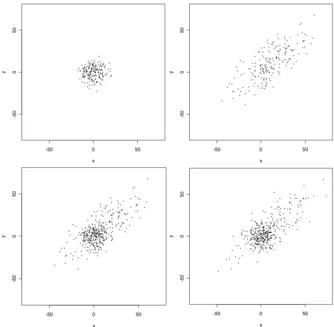
These estimates match the true parameter values very well. Finally, the fitted mixture model was used to generate a new set of 400 observations, which are also displayed in Figure 1 (lower right panel). Upon comparing this display with that for the original set of observations, we see that the fitted model generates data that closely resemble the original simulated data. In this sense, then, the fitted model has excellent predictive power.

Results and Discussion

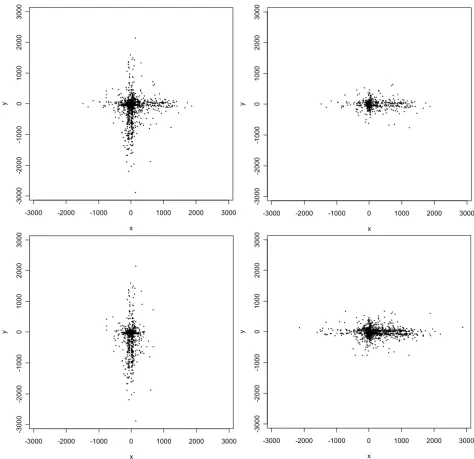
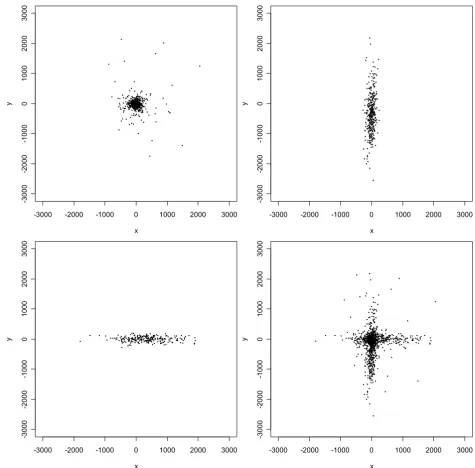
Of the 2354 rural addresses in Carroll County with ortho-photo-derived geocodes, 1423 (60.5%) geocoded using the automated method with a 100%-match criterion. The positional errors (which are two-dimensional vectors) associated with these geocodes ranged in length from a minimum of 3 m to a maximum of 2896 m, with a median of 168 m, and are displayed as points in Figure 2. Interestingly, the errors tend to cluster along the N-S and E-W axial directions in such a way that the overall shape of their distribution, apart from a few outliers, resembles a Greek cross (Figure 2, upper left panel). More errors lie near the center of the cross than near its extremities. More-over, there is a distinct shift in the mean with respect to the origin along each axial direction: along the E-W axis many more errors occur to the east of zero, while along the N-S axis many more errors occur to the south of zero. Close scrutiny also indicates the existence of two parallel "strands" of errors along each axial direction, which strad-dle the axes and are likely due to relatively small offsets of residences from street centerlines. Still more interesting features become apparent upon plotting the errors for the 662 addresses on streets running mainly E-W separately from the errors for the 761 addresses on streets running mainly N-S (Figure 2, upper right and lower left panels). This decomposition shows that while the errors near the cross's center appear to be relatively isotropic, i.e. occur-ring more or less equally often in all directions, those errors away from the center tend to be aligned with the axial orientation of the street on which the corresponding address lies.

ˆ

φ

ˆ

φ

ˆ

φ

ˆ

φ

σX2 σY2

σX2 σY2

ˆ

p µˆ µˆ σˆ_X2

ˆ

σY2 ρˆ

ˆ

p _µˆ _µˆ _σˆ_X2

ˆ

Scatterplot of simulated data from two-component bivariate normal mixture model

Figure 1

Scatterplot of simulated data from two-component bivariate normal mixture model. The upper left panel displays 200 observa-tions from the first component; the upper right panel displays 200 observaobserva-tions from the second component; the lower left panel is a superposition of the two upper panels; and the lower right panel displays a new simulation of 400 observations from the two-component normal mixture model fitted to the data from the original simulation.

-50 0 50

-5

0

0

5

0

x

y

-50 0 50

-5

0

0

5

0

x

y

-50 0 50

-5

0

0

5

0

x

y

-50 0 50

-5

0

0

5

0

x

Scatterplot of positional errors (in meters) for the automated geocodes

Figure 2

Scatterplot of positional errors (in meters) for the automated geocodes. The upper left panel displays the complete data; the upper right panel displays errors for addresses on streets aligned E-W; the lower left panel displays errors for addresses on streets aligned N-S; and the lower right panel is a superposition of the upper right panel and a 90-degree counterclockwise rotation of the lower left panel.

-3000 -2000 -1000 0 1000 2000 3000

-3

000

-20

00

-1

000

0

1

000

2000

3000

x

y

-3000 -2000 -1000 0 1000 2000 3000

-300

0

-200

0

-100

0

0

1000

200

0

3000

x

y

-3000 -2000 -1000 0 1000 2000 3000

-3000

-2

0

00

-1

000

0

1000

2000

300

0

x

y

-3000 -2000 -1000 0 1000 2000 3000

-3

000

-2

00

0

-10

00

0

100

0

2000

3000

x

Manual checking of the fifty largest errors revealed that many were attributable to street segments in the TIGER/ Line file that had correct street names but incorrect address ranges. Others appeared to be attributable to interpolation errors or possibly house address numbering "errors" (i.e. deviations from the distance-from-intersec-tion rule or some other rule that was used when the houses were originally numbered). These database and procedural errors, in combination with the high degree of rectilinearity of the rural road network in Carroll County, produce the distinctive Greek-cross shape of the empirical distribution of positional errors. Outliers from this overall shape appear to be due to either very large offsets (e.g., one house was nearly 800 m from its corresponding street centerline), incorrect TIGER/Line file geometry, or both.

We do not have a ready explanation for the bias with respect to the origin exhibited by the errors. However, the fact that the mean errors are shifted to the east along E-W streets and south along N-S streets, in tandem with the fact that these directions of shift coincide with the directions in which rural house numbers are ascending, suggest that the explanation has something to do with a systematic interpolation or house numbering procedural error. As a follow-up, we computed the mean error for each individ-ual street and found that these means were consistently, in fact invariably, to the east and south. Thus the bias is per-vasive, not merely limited to a few streets.

Owing to the Greek-cross shape of the empirical distribu-tion of the entire set of posidistribu-tional errors, no single bivari-ate normal or t distribution will fit them well, nor for that matter will any elliptical distribution (i.e. a distribution whose contours of equal probability are ellipses). How-ever, the decay in frequency of points with increasing dis-tance from a central location along each axis suggests that a mixture of two or more normal or t distributions, of which at least one is aligned in approximately a N-S direc-tion and at least one other is aligned in approximately an E-W direction, might provide an adequate fit. Conse-quently, normal and t mixtures with various numbers of components were fit to the errors. Values of BIC for each mixture model are given in Table 1a. The results indicate that a three-component mixture fits much better than a two-component mixture, but increasing the number of components beyond three results in marginal improve-ment in fit. The results also show the t mixture model to be superior to the normal mixture model. In light of these results and taking into account the premium on simplicity in measurement-error models, we would select the three-component t model for these errors.

Likelihood-based estimates of the mean vector and covar-iance matrix for the three-component t model are given in Table 2a, and Figure 3 depicts 1423 simulated

observa-tions from the fitted model. (The number of simulated observations was chosen to match the number of real observations so that plots would be directly comparable.) Upon comparing the lower right panel of Figure 3 with the upper left panel of Figure 2, we see that the fitted model reproduces the large-scale features of the positional errors quite well. Furthermore, the parameter estimates and component plots indicate that: (1) the largest compo-nent group consists of errors which are mostly "small" (less than 100 m), relatively isotropic, and centered at the origin, but heavy-tailed (v = 1.6) and thus including some outliers; (2) the other two component groups, comprising relative proportions roughly equivalent to the relative

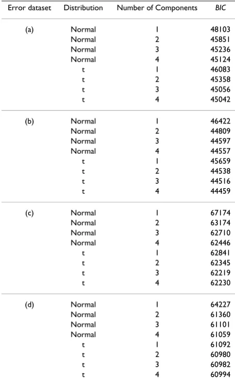
Table 1: Bayesian Information Criteria (BIC) for normal and t mixture models.

Error dataset Distribution Number of Components BIC

(a) Normal 1 48103

Normal 2 45851

Normal 3 45236

Normal 4 45124

t 1 46083

t 2 45358

t 3 45056

t 4 45042

(b) Normal 1 46422

Normal 2 44809

Normal 3 44597

Normal 4 44557

t 1 45659

t 2 44538

t 3 44516

t 4 44459

(c) Normal 1 67174

Normal 2 63174

Normal 3 62710

Normal 4 62446

t 1 62841

t 2 62345

t 3 62219

t 4 62230

(d) Normal 1 64227

Normal 2 61360

Normal 3 61101

Normal 4 61059

t 1 61092

t 2 60980

t 3 60982

t 4 60994

Models with several different numbers of components, were fitted to the following four error datasets: (a) automated geocoding positional errors; (b) automated geocoding positional errors aligned with axial direction of corresponding street segment; (c) E911 positional errors; (d) E911 positional errors aligned with axial direction of

numbers of addresses on N-S and E-W streets, respec-tively, include many errors of intermediate to relatively large size (> 500 m), which are aligned in the N-S and E-W axial directions, respectively, but are lighter-tailed (v = 6.5 and v = 19.6) than the first component and hence rel-atively devoid of outliers; and (3) the means of the second and third components are several hundred meters to the east and south, respectively, of the origin, which is consist-ent with the systematic bias in these directions noted pre-viously.

The lower right panel of Figure 2 displays the "aligned errors," i.e. the errors relative to the axial orientation of the street segment on which the corresponding address lies. Equivalently, the aligned errors are a superposition of the points in the upper right panel and those resulting from a 90-degree counterclockwise rotation of the lower left panel of the same figure. Normal and t mixtures were also fitted to the aligned errors. Values of BIC and likeli-hood-based parameter estimates are given in Tables 1b and 2b, respectively. The results suggest that a two-com-ponent t mixture fits adequately well; that the first compo-nent of this mixture is essentially the same as the first component of the three-component t mixture for the orig-inal errors; and that the second component is essentially the combination of the third component and rotated sec-ond component of the three-component t mixture for the original errors. In fact, BIC for the two-component t mix-ture for the aligned errors is substantially smaller than BIC

for the three-component t mixture for the original errors (Table 1), which indicates that accounting for the orienta-tion of the street on which an address lies results in a more parsimonious model with no reduction in model ade-quacy.

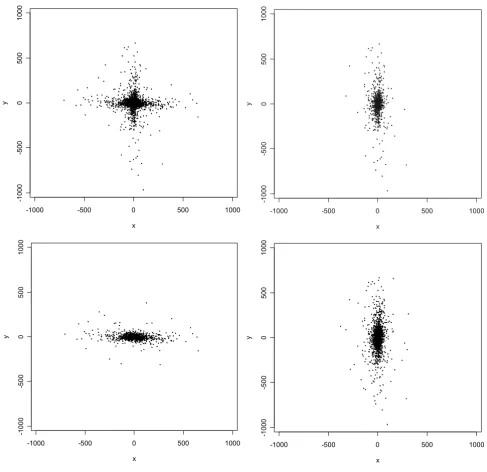
E911 geocoding errors

The positional errors corresponding to the 2354 E911 geocodes (Figure 4) ranged in length from 2 m to 974 m,

with a median of 44 m. Thus, these errors tend to be con-siderably smaller than their automated geocoding coun-terparts. The upper left panel of Figure 4 shows the errors to be arrayed in a Greek cross-like configuration that appears even more pronounced than was the case for the automated geocoding errors, so likewise a single normal or t distribution will not fit well. But once again there is an attenuation in the frequency of points with increasing dis-tance from a central point along each axis, suggesting that a mixture of two or more normal or t distributions might fit the data well. Moreover, the aforementioned central point of the distribution appears to be at or very close to the origin; there is not a mean shift with respect to the ori-gin along each axis as there was for the automated geoco-ding errors. Nor do there appear to be "strands" of points straddling, and running parallel to, each coordinate axis, as there were for the automated geocoding errors. How-ever, there are outliers, and there is an interesting effect of orientational alignment: upon plotting the 1116 addresses on streets aligned mainly E-W separately from the 1238 addresses on streets aligned mainly N-S (Figure 4, upper right and lower left panels), we observe that the errors tend to be aligned orthogonally to the orientation of the street on which the corresponding address lies. This is in sharp contrast to the coincident alignment of automated geocoding errors with the axial orientation of the street, which we noted previously (Figure 2).

The orthogonal alignment of E911 errors occurs as a result of offset errors of substantial magnitude, which in turn are due to the definition of the E911 geocode in rural areas as the coordinates of the intersection of the public road and private road leading to the residence, coupled with the approximate perpendicularity (in most cases) of the angle between the public and private road. The outliers, for the most part, correspond to those cases for which the offset is relatively large and the private road meanders in such a way that a hypothetical line segment connecting the

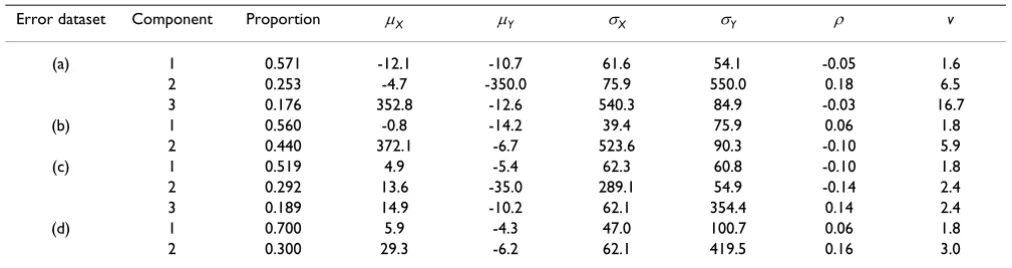
resi-Table 2: Likelihood-based parameter estimates for the best-fitting models.

Error dataset Component Proportion µX µY σX σY ρ v

(a) 1 0.571 -12.1 -10.7 61.6 54.1 -0.05 1.6

2 0.253 -4.7 -350.0 75.9 550.0 0.18 6.5

3 0.176 352.8 -12.6 540.3 84.9 -0.03 16.7

(b) 1 0.560 -0.8 -14.2 39.4 75.9 0.06 1.8

2 0.440 372.1 -6.7 523.6 90.3 -0.10 5.9

(c) 1 0.519 4.9 -5.4 62.3 60.8 -0.10 1.8

2 0.292 13.6 -35.0 289.1 54.9 -0.14 2.4

3 0.189 14.9 -10.2 62.1 354.4 0.14 2.4

(d) 1 0.700 5.9 -4.3 47.0 100.7 0.06 1.8

2 0.300 29.3 -6.2 62.1 419.5 0.16 3.0

Simulated data from the fitted three-component t mixture distribution for the automated geocoding errors

Figure 3

Simulated data from the fitted three-component t mixture distribution for the automated geocoding errors. The upper left panel, upper right panel, and lower left panel correspond to components in order of decreasing p_i; and the lower right panel is their superposition.

-3000 -2000 -1000 0 1000 2000 3000

-3

000

-2

000

-10

0

0

0

1000

2000

3000

x

y

-3000 -2000 -1000 0 1000 2000 3000

-3

000

-2

000

-10

0

0

0

1000

2000

3000

x

y

-3000 -2000 -1000 0 1000 2000 3000

-3

000

-2

000

-1

000

0

1000

2000

3000

x

y

-3000 -2000 -1000 0 1000 2000 3000

-3

000

-2

000

-1

000

0

1000

2000

3000

x

Scatterplot of the positional errors (in meters) for the E911 geocodes

Figure 4

Scatterplot of the positional errors (in meters) for the E911 geocodes. The upper left panel displays the complete data; The upper right panel displays errors for addresses on streets aligned E-W; The lower left panel displays errors for addresses on streets aligned N-S; and the lower right panel is a superposition of the upper right panel and a 90-degree counterclockwise rotation of the lower left panel.

-1000 -500 0 500 1000

-1

000

-500

0

500

1000

x

y

-1000 -500 0 500 1000

-1000

-500

0

5

00

1000

x

y

-1000 -500 0 500 1000

-1

00

0

-50

0

0

50

0

1

0

0

0

x

y

-1000 -500 0 500 1000

-1000

-500

0

500

1000

x

dence to the public road-private road intersection is far from being perpendicular.

Normal and t mixture distributions with various numbers of components were fitted to the E911 errors. Values of

BIC for these fits are listed in Table 1c. On the basis of these values, it appears that a three-component t mixture model provides the best fit; normal models, as well as t models with less than three components, are inadequate. Likelihood-based parameter estimates for the three-com-ponent model are given in Table 2c in order of decreasing

pi, and Figure 5 displays 2354 simulated observations

from the fitted model. Note that the means of all compo-nents lie fairly close to the origin, indicating little system-atic bias in the errors. The estimates and component plots reveal that the component comprising the largest propor-tion (about 52%) consists mostly of relatively small (standard deviation just over 60 m), nearly isotropic errors. The other two components (comprising about 29% and 19% of the errors, respectively) correspond to errors tending to be of larger size (standard deviations of 290 m and 354 m) lying close to the E-W and N-S axial directions, respectively. All three components are quite heavy-tailed, thus outliers occur in all of them. Overall, the simulated data (Figure 5, lower right panel) again seem to reproduce the observed data (Figure 4, upper left panel) quite well.

The lower right panel of Figure 4, which displays all of the E911 errors relative to the axial orientation of the corre-sponding street segment, highlights the aforementioned orthogonality of the errors to street orientation. Normal and t mixtures, once again, were fitted to the errors in this plot. Values of BIC and likelihood-based parameter esti-mates are given in Tables 1d and 2d, respectively. Accord-ing to these results, a two-component t mixture is best-fitting. The component comprising the largest proportion (70%) consists of relatively small errors that are, on aver-age, about twice as large in the orthogonal direction as in the coincident direction. The remaining component con-sists of much larger errors that average about seven times larger in the orthogonal direction than in the coincident direction. Both components are rather heavy-tailed, indi-cating that outliers occur regularly for both.

Conclusion

The major question motivating this investigation was whether one could find useful models for the probability distribution of positional errors associated with geocod-ing, i.e. models that are sufficiently rich to adequately fit various geocoding error datasets yet sufficiently parsimo-nious to be practical for use as measurement-error models for statistical analysis. The answer to this question, based on our findings, is solidly (though not unequivocally) in the affirmative; and the class of models that seems best

suited for the purpose is the class of mixture models of bivariate t distributions. These models can adequately fit such features as clustering along several axial directions, systematic bias in any direction(s), and outliers, all of which occurred in our data; simpler models such as uni-form and normal distributions, which have been used previously for positional errors in spatial data, cannot. Moreover, t mixture models are feasible for use with emerging applications of measurement-error methodol-ogy to epidemiologic research [19,22], provided that they consist of very few components. Based on our results and the other published graphical displays of geocoding errors of which we are aware [12,14], we conjecture that a mix-ture of three (two) t distributions will usually be sufficient for errors (aligned errors) associated with 100%-matched automated geocoding and E911 geocoding, but addi-tional investigations in other places are needed to sub-stantiate this. Positional errors from regions with less rectilinear road networks than Carroll County may not require as many components, as they are less likely to exhibit clustering in the E-W and N-S axial directions; a case in point is displayed in [14]. In some cases a single t distribution or, in the unlikely event of no outliers, a sin-gle normal distribution may even suffice. In any case, if the analyst assumes a t mixture model either with more components than necessary or when a normal mixture model will suffice, the BIC-based model selection proce-dure we have described will (with high probability) point the way to the simpler model.

The one situation we encountered in which mixture mod-els of t distributions proved to be less than fully successful occurred with automated geocoding errors for which an address-matching threshold of less than 100% was used. In this situation, a few small clusters of extremely large errors occurred. Such errors are difficult to model parsi-moniously and, regardless of how they are modeled, will weaken the conclusions made from subsequent statistical inferences using measurement-error methodology. Con-sequently, we recommend using only 100%-matched addresses for spatial epidemiologic analyses.

Simulated data from the fitted three-component t mixture distribution for the E911 geocoding errors

Figure 5

Simulated data from the fitted three-component t mixture distribution for the E911 geocoding errors. The upper left panel, upper right panel, and lower left panel correspond to components in order of decreasing p_i; and the lower right panel is their superposition.

-1000 -500 0 500 1000

-1

00

0

-5

00

0

50

0

1

00

0

x

y

-1000 -500 0 500 1000

-1

00

0

-5

00

0

50

0

1

00

0

x

y

-1000 -500 0 500 1000

-1

00

0

-5

0

0

0

50

0

1

00

0

x

y

-1000 -500 0 500 1000

-1

00

0

-5

0

0

0

50

0

1

00

0

x

Further investigation is currently underway to determine if t mixture models are as useful for positional errors cor-responding to non-rural addresses as they appear to be for rural address positional errors and, if so, how the compo-nents might differ from those for rural addresses. Results from previous studies of positional errors for datasets combining both rural and non-rural addresses [38,10,11,14] suggest strongly that component variances will be smaller for non-rural addresses, but we refrain from predicting how many components may be needed and whether they will prove to be heavy-tailed, mean-shifted away from the origin, etc. Future research may also address the modeling of the probability distribution of positional errors associated with reverse address-matching [39].

How might the methods developed here be adapted to the common situation in which it is not possible to obtain a "gold standard" geocode for each address that has been geocoded via automated geocoding? In some cases it may be feasible to obtain the more accurate geocode for a ran-domly selected portion of the addresses, from which the probability distribution of positional errors associated with automated geocoding may be estimated. This esti-mated distribution may then, as a practical matter, be pre-sumed to apply to the entire set of addresses. In those cases where no sample of positional errors can be obtained, it may still be possible to estimate parameters of a probability distribution of positional errors, provided that a parsimonious model for the true locations of addresses is known (up to its unknown parameters). An illustration of this can be found in [22], and others will be reported elsewhere.

In focusing our attention on geocoding errors, we have ignored the fact that for many studies, automated geocod-ing is incomplete; that is, not all addresses can be assigned point-level spatial coordinates by the software. In fact, it is common in practice for 20% or even as many as 40% of subjects' addresses to fail to geocode using standard soft-ware and street files. For example, Gregorio et al. [40] and Oliver et al. [41] present public health studies in which 14% and 26%, respectively, of addresses could not be assigned a point location via automated geocoding, and for our exclusively rural address dataset this figure was even higher (38%). A statistical analysis based on only the observations that geocode is subject to selection bias [42,41]. However, there is virtually always a reliable coarse (areal-level) measurement, e.g. a zip code, associ-ated with each observation that fails to geocode. Coarse locational data may be combined with the observed point-level data to make valid statistical inferences in the presence of geographic bias via either (a) a coarsened-data maximum likelihood estimation procedure [43], or (b) imputation of a surrogate point location (such as that of a

randomly selected event within the same zip code) for the addresses that do not geocode [44]. Fully satisfactory inference procedures for data whose point locations are ascertained by automated geocoding may require that an inference procedure developed for use with incompletely geocoded data be combined with modifications to account for positional errors.

Authors' contributions

DLZ conceived of this study and drafted the majority of the manuscript. DLZ also directed, and XF performed, the statistical analysis. SM performed the automated geocod-ing and oversaw the orthophoto geocodgeocod-ing of the Carroll County data and contributed to the writing of the Meth-ods section. GR contributed to the writing of several sec-tions.

Acknowledgements

The work of the authors was supported by Centers for Disease Control and Prevention (CDC) Grant Number 3 R01 EH000056-01S1 with the Iowa Department of Public Health (IDPH) and Contract Number 5886CAR02 between the IDPH and the University of Iowa. The views expressed are solely those of the authors and do not represent the views of CDC or IDPH. We thank Carl Wilburn, GIS Coordinator for Carroll County, Iowa for providing address data and E911 geocodes for Carroll County.

References

1. Thomas RW, Ed: Spatial Epidemiology London Papers in Regional Sci-ence 21. London: Pion Ltd; 1990.

2. Elliott P, Wakefield JC, Best NG, Briggs DJ: Spatial Epidemiology: Meth-ods and Applications Oxford, UK: Oxford University Press; 2000. 3. Lawson AB: Statistical Methods in Spatial Epidemiology New York: John

Wiley & Sons; 2001.

4. Waller LA, Gotway CA: Applied Spatial Statistics for Public Health Data

Hoboken, New Jersey: John Wiley & Sons; 2004.

5. Jacquez GM: Current practices in the spatial analysis of can-cer: flies in the ointment. Int J Health Geogr 2004, 3:22. 6. Yang DH, Bilaver LM, Hayes O, Goerge R: Improving geocoding

practices: Evaluation of geocoding tools. J Med Syst 2004, 28:361-370.

7. Kravets N, Hadden WC: The accuracy of address coding and the effects of coding errors. Health Place 2007, 13:293-298. 8. Dearwent SM, Jacobs RR, Halbert JB: Locational uncertainty in

georeferencing public health datasets. J Expo Anal Environ Epide-miol 2001, 11:329-334.

9. Krieger N, Waterman P, Lemieux K, Zierler S, Hogan JW: On the wrong side of the tracts? Evaluating the accuracy of geocod-ing in public health research. Am J Public Health 2001, 91:1114-1116.

10. Bonner MR, Han D, Nie J, Rogerson P, Vena JE, Freudenheim JL: Posi-tional accuracy of geocoded addresses in epidemiologic research. Epidemiology 2003, 14:408-412.

11. Whitsel EA, Rose KM, Wood JL, Henley AC, Liao D, Heiss G: Accu-racy and repeatability of commercial geocoding. Am J Epide-miol 2004, 160:1023-1029.

12. Whitsel EA, Quibrera PM, Smith RL, Catellier DJ, Liao D, Henley AC, Heiss G: Accuracy of commercial geocoding: assessment and implications. Epidemiologic Perspectives and Innovations 2006, 3:8. 13. Ward MH, Nuckols JR, Giglierano J, Bonner MR, Wolter C, Airola M,

Mix W, Colt JS, Hartge P: Positional accuracy of two methods of geocoding. Epidemiology 2005, 16:542-547.

14. Cayo MR, Talbot TO: Positional error in automated geocoding of residential addresses. Int J Health Geogr 2003, 2:10.

Publish with BioMed Central and every scientist can read your work free of charge "BioMed Central will be the most significant development for disseminating the results of biomedical researc h in our lifetime."

Sir Paul Nurse, Cancer Research UK

Your research papers will be:

available free of charge to the entire biomedical community

peer reviewed and published immediately upon acceptance

cited in PubMed and archived on PubMed Central

yours — you keep the copyright

Submit your manuscript here:

http://www.biomedcentral.com/info/publishing_adv.asp

BioMedcentral 16. Jacquez GM, Waller LA: The effect of uncertain locations on

dis-ease cluster statistics. In Quantifying Spatial Uncertainty in Natural Resources: Theory and Applications for GIS and Remote Sensing Edited by: Mowrer HT, Congalton RG. Chelsea, Michigan: Arbor Press; 2000:53-64.

17. Zimmerman DL: Statistical methods for incompletely and incorrectly geocoded cancer data. In Geocoding Health Data: The Use of Geographic Codes in Cancer Prevention and Control, Research and Practice Edited by: Rushton G, Armstrong MP, Gittler J, Greene BR, Pavlik CE, West MM, Zimmerman DL. Boca Raton, Florida: CRC Press in press.

18. Burra T, Jerrett M, Burnett RT, Anderson M: Conceptual and prac-tical issues in the detection of local disease clusters: a study of mortality in Hamilton, Ontario. The Canadian Geographer

2002, 46:160-171.

19. Diggle PJ: Point process modelling in environmental epidemi-ology. In Statistics for the Environment Edited by: Barnett V, Turkman KF. New York: John Wiley & Sons; 1993:89-110.

20. Gabrosek J, Cressie N: The effect on attribute prediction of location uncertainty in spatial data. Geographical Analysis 2002, 34:262-285.

21. Cressie N, Kornak J: Spatial statistics in the presence of loca-tion error with an applicaloca-tion to remote sensing of the envi-ronment. Statistical Science 2003, 18:436-456.

22. Zimmerman DL, Sun P: Estimating spatial intensity and varia-tion in risk from locavaria-tions subject to geocoding errors. Tech-nical report #363, Department of Statistics and Actuarial Science, University of Iowa 2006:1-19 [http://www.stat.uiowa.edu/techrep/ tr363.pdf].

23. ArcGIS 9: Geocoding Rule Base Developers Guide Redlands, California: Earth Sciences Research Institute; 2003.

24. Postal Addressing Standards-Publication 28: United States Postal Service 2000 [http://pe.usps.com/cpim/ftp/pubs/Pub28/ pub28.pdf].

25. Natural Resources Geographic Information Systems Library [http://www.igsb.uiowa.edu/nrgislibx/]

26. Barber JJ, Gelfand AE, Silander JA: Modeling map positional error to infer true feature location. Canadian Journal of Statistics in press.

27. Everitt BS, Hand DJ: Finite Mixture Distributions London: Chapman and Hall; 1981.

28. Titterington DM: Statistical Analysis of Finite Mixture Distributions Chich-ester: John Wiley & Sons; 1985.

29. McLachlan GJ, Basford KE: Mixture Models New York: Marcel Dekker; 1988.

30. Basford KE, McLachlan GJ: Likelihood estimation with normal mixture models. Applied Statistics 1985, 34:282-289.

31. Dempster AP, Laird NM, Rubin DB: Maximum likelihood from incomplete data via the EM algorithm (with discussion). Jour-nal of the Royal Statistical Society Series B 1977, 39:1-38.

32. Kiefer J, Wolfowitz J: Consistency of the maximum likelihood estimates in the presence of infinitely many incidental parameters. Annals of Mathematical Statistics 1956, 27:887-906. 33. Kiefer NM: Discrete parameter variation: efficient estimation

of a switching regression model. Econometrica 1978, 46:427-434. 34. EMMIX [http://www.maths.uq.edu.au/~gjm/emmix/emmix.html] 35. McLachlan GJ, Krishnan T: The EM Algorithm and Extensions New York:

John Wiley & Sons; 1997.

36. Peel D, McLachlan GJ: Robust mixture modelling using the t dis-tribution. Statistics and Computing 2000, 10:339-348.

37. Burnham KP, Anderson DR: Model Selection and Multi-Model Inference

New York: Springer-Verlag; 1998.

38. McElroy JA, Remington PL, Trentham-Dietz A, Robert SA, Newcomb PA: Geocoding addresses from a large population-based study: lessons learned. Epidemiology 2003, 14:399-407.

39. Curtis A, Mills J, Leitner M: Spatial confidentiality and GIS: re-engineering mortality locations from published maps about Hurricane Katrina. Int J Health Geogr 2006, 5:44.

40. Gregorio DI, Cromley E, Mrozinski R, Walsh SJ: Subject loss in spa-tial analysis of breast cancer. Health Place 1999, 5:173-177. 41. Oliver MN, Matthews KA, Siadaty M, Hauck FR, Pickle LW:

Geo-graphic bias related to geocoding in epidemiologic studies.

Int J Health Geogr 2005, 4:29.

42. Gilboa SM, Mendola P, Olshan AF, Harness C, Loomis D, Langlois PH, Savitz DA, Herring AH: Comparison of residential geocoding

methods in population-based study of air quality and birth defects. Environ Res 2006, 101:256-262.

43. Zimmerman DL: Estimating spatial intensity and variation in risk from locations coarsened by incomplete geocoding.

Technical report #362, Department of Statistics and Actuarial Science, Uni-versity of Iowa 2006:1-28 [http://www.stat.uiowa.edu/techrep/ tr362.pdf].

44. Boscoe F: The science and art of geocoding: Tips for improv-ing match rates and handlimprov-ing unmatched cases in analysis. In