Please cite this article in press as: Govindaraju S, Rudravaram VV. Testing the significance of crossover receiver operating characteristic curves in the presence of multiple markers. J Biostat Epidemiol. 2016; 2(4): 164-72
J Biostat Epidemiol. 2016; 2(4): 164-72.
Original Article
Testing the significance of crossover receiver operating characteristic curves in
the presence of multiple markers
Sameera Govindaraju1, Vishnu Vardhan Rudravaram1*
1
Department of Statistics, Ramanujan School of Mathematical Sciences, Pondicherry University, Puducherry, India
ARTICLE INFO ABSTRACT
Received 18.04.2016 Revised 27.07.2016 Accepted 19.10.2016 Published 01.12.2016
Background & Aim: In multivariate receiver operating characteristic (MROC) curve analysis, comparing two tests is usually done by means of area under the curve (AUC‟s) and sensitivities. However, the existing procedures have not addressed the issue of comparing two MROC curves when they cross each other.
Methods & Materials: A modified version of AUC (mAUC) under MROC setup is proposed to address the above-mentioned problem. It is also shown that mAUC performs better than AUC. The performance of mAUC in the aspect of crossover curves is supported by a real dataset and simulation studies at different sample sizes.
Results: Two real datasets, namely, Intra Uterine Growth Restricted Fetal Doppler Study (IUGRFDS) and Indian liver patient (ILP) datasets are used and apart from these simulation studies are also carried out to observe the effect of sample size. These mAUC‟s are then compared with each other to show that difference exists between two curves while comparing AUC‟s cannot identify the true difference existing between them. With respect to IUGRFDS dataset, MROC curves of the diagnostic procedures middle cerebral artery and cerebroplacental ratio cross each other and are found to be similar when their AUC‟s and mAUC‟s are compared. In ILP dataset, the extent of correct classification achieved in the case of males is shown to be better than that of females when mAUC‟s at 0.5 and 0.8 are compared.
Conclusion: It is observed that the mAUC‟s are competent in identifying the true difference between the crossover MROC curves when the sample size is adequate, and the λ values are 0.5 and 0.8 but not 0.3.
Key words: Multivariate; Area under the curve; Crossing-over, Multivariate receiver operating characteristic curve
Introduction
1A number of classification techniques were developed over the decades to accommodate the need for identifying an individual‟s status in a variety of fields such as psychology, banking, forensics, and medicine. The field of medicine adapted one such classification technique known as the receiver operating characteristic (ROC) curve analysis. One of the major uses of ROC
* Corresponding Author: Vishnu Vardhan Rudravaram, Postal Address: Department of Statistics, Pondicherry University, Puducherry, India. Email: [email protected]
was further demonstrated to be comfortable to use over discriminant analysis as it does not impose restrictions on covariance matrices.
In multivariate classification, attention is required for those reference values of markers which provide at least a moderate amount of classification. In usual context of assessing the performance of a test, scores which are nearer to reference value are given the same amount of weightage as that of the scores farther from reference value. The area under the curve (AUC) so computed will be contaminated, and the true accuracy or the actual performance will be masked. This misleads the interpretation of the measures of ROC as well as the optimal threshold. In general, let us consider two tests A and B for better identification of a particular abnormality in individuals. Suppose that the curves of tests A and B cross each other and have at most similar accuracies. Under these circumstances, it is very difficult to notify a better test which has more ability to distinguish status of individuals. To resolve this issue, a new testing procedure is given in a parametric sense which makes use of the modified version of AUC rather than the conventional AUC of MROC curve proposed by Sameera et al. (4). Further, the role of sample size in distinguishing the crossover MROC curves is also considered, and numerical illustrations are accommodated by both real and simulated environments.
Methods
Let X (healthy, H) and Y (diseased, D) denote two p-variate normal random vectors such that X~MVN(µH, ΣH) and Y~MVN(µD, ΣD) where µH
and µD are mean vectors and ΣH and ΣD are
covariance matrices. The probability density function of the two populations is given by,
( | )
( ) ⁄ | | { (
) ( )}
The MROC model and its AUC is given by Sameera et al. (4) is
( ) ( ( ) ( )⁄ ( ( ))
( )⁄ ) (1)
( ( )
[ ( ) ]⁄ ) (2)
Here, b = [tΣD + (1−t) ΣH ]−1 (μD-μH);0 < t < 1
where the value of t is determined through trial and error, and c denotes the score values from both populations.
In general, testing the significance of single AUC against AUC0 = 0.5 or comparing the
AUC‟s of two MROC curves is the problem of interest. Vardhan et al. (5) addressed this problem by proposing inferential procedures based on AUC‟s and sensitivities. The Z-statistic for comparing AUC‟s of two MROC curves is
( ) ( )
√ ( ( )) ( ( ))
(3)
The procedures proposed by Vardhan et al. (5) failed to address the issue of crossover ROC curves. This leads to the development of a new testing procedure to compare crossover curves, resulted in the concept of modified AUC (mAUC) of MROC curve.
mAUC: AUC is the probability that an individual/object from group “D” has a score greater than individual/ object from group “H.” One small drawback with this definition is that it does not take into account the amount by which the scores of group “D” and group “H” differ. To overcome this, a weight is assigned to those scores where the difference between scores is comparatively small. mAUC was defined probabilistically by Yu et al. (6) under univariate setup as weighted sum of two AUC‟s.
i.e., mAUC = P(Y−X > δ) + (1−λ) P (0<Y−X≤δ)
⟹mAUC = (1−λ)P(Y > X) + λP(Y > X + δ)
the conventional AUC. Using the above probabilistic notations, mAUC is derived for MROC model and is given as:
( ) ( ( )
[ ( ) ] ⁄ )
( ( )
[ ( ) ] ⁄ ) (4)
In equation (4), the values of parameters λ and δ are to be chosen in such a way that the true accuracy of a test can be extracted by minimizing the effect of nearby points of the threshold. If λ value is taken to be 0, mAUC reduces to AUC, and if it is taken as 1, the probability P(Y > X + δ) is only taken into account. Any value of λ > 1 would result in making the probability P(0 < Y − X ≤ δ) value a penalty. Hence, a reasonable choice for λ lies in the range (0, 1), larger the λ value lower the importance on AUC. Further, a possible value of δ can be chosen using the following result.
Results
The upper bound for mean vector can be
shown as ̅ √ ( ) ( ) ( )( ) where
n is the number of samples, k is the number of markers, and b'Sb is the quadratic form.
Proof: A quadratic form defined by T2 has an upper bound say d2 (7), that is,
( ̅ ) ( ̅ )
Where, d is a constant. Then for every b, the above equation implies that:
( ̅ )
And this reduces to
̅ √ ̅ √
Choosing ( )( ) ( ) gives intervals
that contain b' μ for all b. Considering the upper bound from above expression and successively choosing b' = (1,0,…0) b' = (0,1,…0) and so on till b' = (0,0,…1) we get,
̅ √ ( )( ) ( )√
̅ √ ( )( ) ( )√
̅ √ ( )( ) ( )√
Holding with confidence coefficient (1−α). The difference μi−μk corresponding to
b' = (0,…0,bi,0…0,bk where bi = 1 and bk = −1
can be computed without modifying the confidence coefficient (1−α). Then b' Sb = sii−2sik + skk and we get,
̅ ̅ √ ( )( ) ( )√
Along similar lines, any choice of „b‟ provides a linear combination which does not affect the confidence coefficient, thus implying that,
̅ √ ( ) ( ) ( )
The RHS of the above expression is the upper bound of the mean vector.
Based on the above result, the parameter δ
can be chosen as √ ( ( ) ) ( )( )
the main reason for this choice of δ is that the upper bound for the mean vector of healthy population is
̅ √ ( ( ) ) ( )( ) . If an
observed score is larger than this upper bound, then individual‟s status can be affirmatively called true positive (diseased).
Let there be two tests A and B with a crossover behavior and their accuracies are mAUC(1) and
mAUC(2). The testing procedure proposed to test
the hypothesis H0: mAUC(1)=mAUC(2) against
H1: mAUC(1)≠mAUC(2) for identifying the
difference between two cross over MROC curves is defined as:
( ) ( )
√ ( ( )) ( ( ))
The variance of mAUC expression cannot be derived explicitly and hence the concept of bootstrapping is used. If “B” bootstraps are generated from the dataset, then the estimate and variance of mAUC are given as:
∑ (6)
( )
∑ ( )
(7)
Where ( ( )) can be
estimated using bootstrapping. The Z value follows standard normal distribution asymptotically. The asymptotic confidence interval for mAUC can be obtained using ( )√ ( ).
Numerical Illustrations
For demonstrating the proposed methodology is supported using a real dataset, namely, Intra Uterine Growth Restricted Fetal Doppler Study (IUGRFDS) dataset (5) and Indian liver patient (ILP) dataset (8). Further, simulation studies are also carried out to observe the effect of sample size. The computations of mAUC and its confidence intervals are given at λ = {0.3, 0.5, 0.8} for illustration purposes. These mAUC‟s are then compared with each other to show that difference exists between two curves while comparing AUC‟s cannot identify the true difference existing between them.
Real Datasets
IUGRFDS dataset: The dataset IUGRFDS contains data collected from two independent diagnostic procedures cerebroplacental ratio (CPR) and middle cerebral artery (MCA). Here, comparison is to be made between CPR and MCA procedures to find out which procedure is
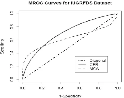
better in identifying the sufficient blood flow from the mother to baby. The AUC‟s and mAUC‟s of CPR and MCA along with their corresponding Z statistic value are computed and reported in table 1. The crossover MROC curves for CPR and MCA procedures are shown in figure 1.
For the three values of λ, mAUC values are lower than that of AUC values. This is due to the fact that the mAUC expression takes the values of λ into account which results in assigning an appropriate weight to those scores that are closer to the threshold for extracting the true accuracy of a diagnostic procedure. The results portrayed in table 1 depict that both the procedures; CPR and MCA are equally effective in identifying the blood flow from mother to baby.
Figure 1. Crossover multivariate receiver operating characteristic curves for Intra Uterine Growth Restricted Fetal Doppler Study dataset
Even though the proposed mAUC is meant to identify the true difference between crossover MROC curves; the above results do not signify the difference between the procedures. This leads to having a susceptible thinking to focus on the effect of sample size on the proposed testing procedure.
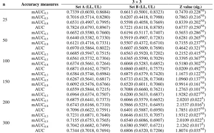
Table 1. Comparison between CPR and MCA using mAUC
Measure CPR (LL, UL) MCA (LL, UL) Z value (sig.)
mAUC0.3 0.6551 (0.5196, 0.7815) 0.5902 (0.5034, 0.7254) 0.8008 (0.212NS) mAUC0.5 0.6369 (0.5106, 0.7631) 0.5774 (0.4453, 0.7090) 0.7070 (0.239
NS ) mAUC0.8 0.6095 (0.4817, 0.7577) 0.5581 (0.4558, 0.7032) 0.5777 (0.282NS) AUC 0.6824 (0.5702, 0.7906) 0.6095 (0.5329, 0.7139) 0.9536 (0.170NS)
Table 2. Comparison between males and females using mAUC
Measure Males (LL, UL) Females (LL, UL) Z value (sig.) mAUC0.3 0.6989 (0.6721, 0.7241) 0.6116 (0.5252, 0.7025) 1.8327 (0.033NS) mAUC0.5 0.6908 (0.6597, 0.7230) 0.5912 (0.5118, 0.6697) 2.0605 (0.019*) mAUC0.8 0.6788 (0.6571, 0.7124) 0.5606 (0.4512, 0.6598) 2.3824 (0.009*) AUC 0.7109 (0.6759, 0.7297) 0.6422 (0.5591, 0.7203) 1.4726 (0.070NS)
mAUC: Modified area under the curve, NS: Nonsignificant, AUC: Area under the curve
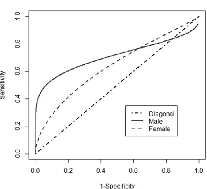
ILP dataset: The ILP dataset is divided into two sets based on gender as males and females. MROC curves of males and females are then compared to check if classification is better in one gender compared to the other. The mAUC and AUC values are calculated for both datasets and placed in table 2 along with their Z values and significance.
A better classification is seen in males than females when mAUC‟s obtained at λ = 0.5 and λ = 0.8 are compared. However, the Z value obtained for AUC‟s shows no difference between the curves indicating that the influence of values close to the threshold is high when comparing the curves that cross each other. The mAUC‟s at λ = 0.3 also do not differ from each other indicating that the weightage given to threshold values should not be too less. The MROC curves obtained for males and females can be seen in figure 2.
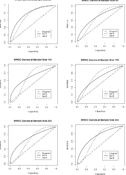
Simulation studies: For simulation purpose, two sets A and B of trivariate normal distribution are considered. The mean vectors and covariance matrices for sets A and B are reported in table 3. Entire simulations are carried out at nD = nH =
n = {25, 50, 100, 150, 200, 300}.
Table 4 summarizes mAUC and AUC values and their corresponding Z statistic for sets A and B. These simulations are carried out to address the points: the first one is to address the presence of λ influences mAUC making it smaller than AUC, and further implies that mAUC provides „true‟ information or accuracy about the test. This means that the test scores which are nearby
the classifier rule are given smaller weightage which leads to the correct identification of true positives. The second is to focus on the effect of sample size in the comparison of crossover curves to provide an evidence that mAUC performs better than AUC in distinguishing the two curves for giving out a better one when there is an adequate sample size.
Figure 2. Crossover multivariate receiver operating characteristic curves for Indian liver patient dataset
Even though there is a discrepancy between AUC‟s of set A and set B, Z statistic results-in insignificant outcome suggesting that AUC is not helpful in identifying the better curve. A true distinction is noticed at sample sizes n = 200, 300 for λ values 0.5 and 0.8 but not 0.3.
Table 3. Mean vectors and covariance matrices for simulations
Set µD µH ΣD ΣH
A
( ) (
) (
) (
)
B
( ) (
) (
) (
Table 4. mAUC’s and AUC’s of Simulated data along with Z values
n Accuracy measures 3 × 3
Set A (LL, UL) Set B (LL, UL) Z value (sig.)
25
mAUC0.3 0.7339 (0.6030, 0.8684) 0.6613 (0.5001, 0.8323) 0.7470 (0.228NS) mAUC0.5 0.7016 (0.5714, 0.8280) 0.6207 (0.4418, 0.7988) 0.7863 (0.216NS) mAUC0.8 0.6531 (0.4907, 0.7995) 0.5598 (0.4058, 0.7669) 0.8339 (0.202NS) AUC 0.7824 (0.6793, 0.8967) 0.7221 (0.6118, 0.8785) 0.6737 (0.250NS)
50
mAUC0.3 0.6652 (0.5580, 0.7660) 0.6194 (0.5117, 0.7407) 0.5653 (0.286 NS
) mAUC0.5 0.6440 (0.5382, 0.7330) 0.5919 (0.4907, 0.7283) 0.6281 (0.265NS) mAUC0.8 0.6121 (0.4716, 0.7331) 0.5507 (0.4372, 0.6710) 0.7155 (0.237
NS ) AUC 0.6970 (0.5864, 0.8022) 0.6607 (0.5609, 0.7690) 0.4642 (0.321NS)
100
mAUC0.3 0.6685 (0.5947, 0.7515) 0.6563 (0.5920, 0.7202) 0.2152 (0.415 NS
) mAUC0.5 0.6561 (0.5732, 0.7304) 0.6365 (0.5590, 0.7029) 0.3395 (0.367NS) mAUC0.8 0.6374 (0.5661, 0.7264) 0.6068 (0.5283, 0.6852) 0.5180 (0.302
NS ) AUC 0.6871 (0.6162, 0.7507) 0.6860 (0.6051, 0.7575) 0.0209 (0.492NS)
150
mAUC0.3 0.6384 (0.5746, 0.6984) 0.6875 (0.6379, 0.7420) 1.1673 (0.122 NS
) mAUC0.5 0.6267 (0.5641, 0.6817) 0.6733 (0.6128, 0.7368) 1.0960 (0.137NS) mAUC0.8 0.6092 (0.5476, 0.6766) 0.6520 (0.6011, 0.7060) 0.9914 (0.161NS) AUC 0.6559 (0.5844, 0.7215) 0.7088 (0.6660, 0.7621) 1.2763 (0.101NS)
200
mAUC0.3 0.6964 (0.6374, 0.7507) 0.6200 (0.5633, 0.6837) 1.9282 (0.027 NS
) mAUC0.5 0.6875 (0.6441, 0.7373) 0.6066 (0.5579, 0.6652) 2.0203 (0.022S) mAUC0.8 0.6743 (0.6166, 0.7310) 0.5866 (0.5251, 0.6493) 2.1537 (0.016S) AUC 0.7096 (0.6622, 0.7591) 0.6401 (0.5887, 0.6950) 1.7851 (0.037NS)
300
mAUC0.3 0.7231 (0.6871, 0.7640) 0.6646 (0.6133, 0.7057) 1.9312 (0.027NS) mAUC0.5 0.7155 (0.6753, 0.7565) 0.6540 (0.6086, 0.6907) 2.0109 (0.022
S ) mAUC0.8 0.7042 (0.6682, 0.7499) 0.6380 (0.5907, 0.6721) 2.1262 (0.017S) AUC 0.7344 (0.7018, 0.7694) 0.6806 (0.6320, 0.7206) 1.8074 (0.035NS)
mAUC: Modified area under the curve, NS: Nonsignificant, S: Significant, AUC: Area under the curve This implies that the weightage given to
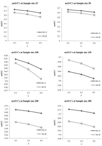
scores close to threshold should be neither too small nor too large. A small weightage would make it difficult to identify the difference between the curves while a large weightage would reduce the mAUC value considerably. The graphs in figure 3 show that as the sample size increases the distance between the mAUC‟s of set A and set B increase. The distance between mAUC‟s of sets A and B is very low for sample sizes 25, 50, and 100. A better distance is observed between the mAUC‟s for sample sizes 150, 200, and 300. However, the results pertaining to mAUC detail out true discrepancy between sets A and B resulting that set A out performs set B. The confidence intervals obtained for three λ values show that tighter bounds are achieved for λ = 0.8 followed by 0.5 and 0.3.
The above simulations are portrayed in terms of MROC curves that cross each other depicting the behavior of the curves at considered sample sizes (figure 4). A simple observation noted with these simulations is that the curves tend to possess varying shapes as the sample size varies.
Discussion
Figure 3. Modified area under the curve for simulated datasets at varying λ 0 0.1 0.2 0.3 0.4 0.5 0.6 0.7 0.8
0.3 0.5 0.8
m
A
U
C
λ
mAUC's at Sample size 25
Set A Set B 0 0.1 0.2 0.3 0.4 0.5 0.6 0.7
0.3 0.5 0.8
m
A
U
C
λ
mAUC's at Sample size 50
Set A Set B 0.57 0.58 0.59 0.6 0.61 0.62 0.63 0.64 0.65 0.66 0.67 0.68
0.3 0.5 0.8
m
A
U
C
λ
mAUC's at Sample size 100
Set A Set B 0.56 0.58 0.6 0.62 0.64 0.66 0.68 0.7
0.3 0.5 0.8
m
A
U
C
λ
mAUC's at Sample size 150
Set A Set B 0.52 0.54 0.56 0.58 0.6 0.62 0.64 0.66 0.68 0.7 0.72
0.3 0.5 0.8
m
A
U
C
λ
mAUC's at Sample size 200
Set A Set B 0.58 0.6 0.62 0.64 0.66 0.68 0.7 0.72 0.74
0.3 0.5 0.8
m
A
U
C
λ
mAUC's at Sample size 300
Further, simulation studies were conducted to observe whether there is an effect of sample size on mAUC in distinguishing two crossover curves.
Conclusion
From the results obtained through simulations, it is observed that the mAUC‟s are competent in identifying the true difference between the crossover MROC curves when the sample size is adequate, and the λ values are 0.5 and 0.8 but not 0.3. This implies that the λ value should not be too small to acquire true information about the curve. Lower λ values mean that the values close to the threshold are too suppressed to contribute toward classification. On the whole, observations from these experimentations support in claiming that mAUC can be considered as an alternative to AUC in the context of crossover curves.
Conflict of Interests
Authors have no conflict of interests.
Acknowledgments
The author, Sameera G, would like to acknowledge the Department of Science and Technology for supporting her research through a fellowship under DST-INSPIRE programme (IF130958).
References
1. Liu A, Schisterman EF, Zhu Y. On linear
combinations of biomarkers to improve diagnostic accuracy. Stat Med 2005; 24(1): 37-47.
2. Su JQ, Liu JS. Linear combinations of multiple diagnostic markers. J Am Stat Assoc 1993; 88(424): 1350-5.
3. Johnson RA, Wichern DW. Applied multivariate statistical analysis. Upper Saddle River, NJ: Pearson Prentice Hall; 2007.
4. Pepe MS, Thompson ML. Combining diagnostic test results to increase accuracy. Biostatistics 2000; 1(2): 123-40.
5. Sameera G, Vardhan RV, Sarma KV. Binary classification using multivariate receiver operating characteristic curve for continuous data. J Biopharm Stat 2016; 26(3): 421-31.
6. Vardhan RV, Sameera G, Chandrasekharan PA, Beere T. Inferential procedures for comparing the accuracy and intrinsic measures of multivariate receiver operating characteristic (MROC) Curve. Int J Stat Med Res 2015; 4(1): 87-93.
7. Yu W, Chang YcI, Park E. A modified area under the ROC curve and its application to marker selection and classification. J Korean Stat Soc 2014; 43(2): 161-75.