Please cite this article as: Z. Abtahi, R. Sahraeian, D. Rahmani, A New Approach Generating Robust and Stable Schedules in m-Machine Flow Shop Scheduling Problems: A Case Study, International Journal of Engineering (IJE), IJE TRANSACTIONS B: Applications Vol. 33, No. 2, (February 2020) 293-303
International Journal of Engineering
J o u r n a l H o m e p a g e : w w w . i j e . i r
A New Approach Generating Robust and Stable Schedules in
m-Machine Flow Shop
Scheduling Problems: A Case Study
Z. Abtahia, R. Sahraeian*a, D. Rahmanib
a Department of Industrial Engineering, College of Engineering, Shahed University, Tehran, Iran b Department of Industrial Engineering, K.N. Toosi University of Technology, Tehran, Iran
P A P E R I N F O
Paper history: Received 12 March 2019
Received in revised form 10 October 2019 Accepted07November 2019
Keywords:
Machine Breakdowns Robustness Scheduling Stability
Uncertain Flow Shop System
A B S T R A C T
This paper considers a scheduling problem with uncertain processing times and machine breakdowns in industriall/office workplaces and solves it via a novel robust optimization method. In the traditional robust optimization, the solution robustness is maintained only for a specific set of scenarios, which may worsen the situation for new scenarios. Thus, a two-stage predictive algorithm is proposed to efficiently handle the uncertainties and find robust and stable solutions. The first stage creates robust solutions and ensures their stability in the new scenarios. The second stage proposes a novel stability measure to proactively offset the effects of the machine breakdowns of the former stage. Moreover, a tri-component measure based on efficiency, robustness, and stability is proposed which aims to create a realistic schedule to satisfy the customers, manufacturers, and the staff. To meet the customer’s requirements, the robustness measure is defined based on the tardiness and the delivery dates of jobs. Finally, the proposed algorithm is applied to a case study, and the findings are compared with the empirical data. The results emphasize the superiority of the proposed technique in satisfying the customers, staff, and increasing the profitability and accountability of the company.
doi: 10.5829/ije.2020.33.02b.14
1. INTRODUCTION1
The shop scheduling literature includes a large number of papers dealing with the classical permutation flowshop scheduling (FSS) problem, in which a set of jobs must be processed on the series of machines in the same order. In the majority of these researches, no disruption is assumed in the production systems, and the classical performance measures are usually optimized under deterministic assumptions [1]. However, in practice, many disruptions may occur e.g. machine breakdowns, uncertain processing times, the arrival of new jobs, etc. Two sources of uncertainty are considered in this paper; the unexpected breakdowns of the first machine and the uncertain processing times of all the jobs. Due to the uncertainties, it is expected to be some deviations between the real schedule (i.e. the schedule that is carried out on the shop floor), and the initial one (i.e. the schedule planned at the beginning of the scheduling horizon). The comparison of the real schedule with the
*Corresponding Author Email: [email protected] (R.Sahraeian)
to defining very different solutions as robust". In other words, the schedule robustness is guaranteed only for the set of considered scenarios and may fail when dealing with a new scenario. Therefore it is crucial to identify a robust and stable solution in the face of new scenarios. In this paper, a predictive two-stage algorithm is proposed that in its first stage, a robust schedule is produced and then evaluated for its stability against a new job processing times' scenario. In almost all of the robustness oriented studies, exposure to machine failure has been done with the reactive approach or in the reactive phase of the hybrid approaches. In the reactive scheduling methods (e.g. rescheduling), especially in the case of big problems, it takes a long time to deal with the uncertain conditions. Predictive scheduling methods can overcome this problem by proactively preparing for any possible occurrence of such uncertain conditions [6]. Ergo, in this paper, exposer to machine failure has been done with the predictive approach. Idle time insertion has been a common strategy to handle the effect of breakdown disruptions (e.g. see [4, 5]). This method faces two challenges, which are finding the optimal amount and the appropriate position to insert the buffer times [7]. In the second stage of our proposed algorithm, a linear optimization method is employed to overcome these challenges. A new surrogate measure is proposed to enhance the solution robustness by interfering with the probability of machine breakdown during the job processing times. This linear programming model simultaneously optimizes the proposed surrogate measure of solution robustness, and quality robustness to determine the proper position and the amount of buffer times. One of the essential prerequisites of practical scheduling is to meet customer, manufacturer and staff requirements simultaneously. This is addressed in this paper by defining a tri-component performance measure of robustness, efficiency, and stability. Due to the important role of customer-agreed delivery deadlines in manufacturing systems, tardiness-based performance measures have been the focus of attention. However, tardiness is considered as the performance measure in only 5 percent of the related studies [8]. In this paper, the total real tardiness of jobs is considered a robustness measure. Finally, a case study is presented to compare the performance of the proposed method with the empirical method used in the company based on a tri-criteria objective measure of robustness, stability, and efficiency. Thus, the main contributions of this paper are as follows: - An m-machine FSS problem under two sources of
uncertainty is considered.
- A triple scale is proposed to simultaneously meet the needs of the customer, producer, and worker. - An appropriate predictive method to handle the
uncertainty of the job processing times and machine breakdown is proposed.
- The stability of the robust solution in the face of a new job processing time scenario is ensured.
- An innovative surrogate measure is proposed to enhance solution robustness.
A linear programming model is proposed to determine the proper position and the amount of the buffer times.
This paper is organized as follows. In section 2, the related literature is reviewed. A brief description of the robust optimization approach and the proposed predictive algorithm are presented in section 3. The case study and the computational results are provided in section 4. Finally, the conclusion and the suggestions for future researches are discussed in section 5.
2. LITERATURE REVIEW
In this paper uncertainty oriented flow shop scheduling problem studies in 2000-2019 are reviewed focusing on the source of uncertainty, The purpose of scheduling, and the approach in counter with uncertainty and the results are summarized in this section. "Flow shop" is considered as a keyword in the title of studies, and "robustness/ robust", "stability/ stable", "uncertainty/ uncertain job processing time/ machine breakdown" are considered as keywords in the body of the studies.
probability of not exceeding from the specified threshold (e.g. [10, 11]). Considering an identical threshold is one of the gaps in this type of researches. Approximately in all of the scenario-based robustness oriented flow shop schedule studies, dual or multiple performance measures of efficiency, robustness and/ or stability were used. In all of these studies, the basis for constructing robustness and stability measures has been Cmax (e. g. see [1, 9, 15, 16]). According to the literature [17], failure is considered for only one machine even in recent papers. However, in some related studies [1], the failure is considered for more than one machine. Also, the repair time can be varied, which is not the case in most related articles [18]. In the face of machine breakdown disruption, predictive [2, 4, 6] or reactive [1] rescheduling methods have been addressed in the literature. The non-idle time insertion methods such as time-consuming simulation-based methods proposed in some studies in the face of machine breakdown disruption [3, 7]. Buffer time insertion method has been a common predictive strategy to counter the effect of breakdowns [4], but it faces two problems; how to find the optimal amount and the appropriate position to insert the buffer times. Briskorn et al. [18] analyzed the allocation of idle times in a single-machine environment. It can be gathered from the literature that in most of the related studies:
- One source of uncertainty has been considered. - Efficiency, stability, and robustness were often
considered separately except in some recent papers [1, 15].
- The stability of the robust solution in the face of new scenarios has not been investigated.
- None of the measures of robustness and efficiency are defined based on the tardiness of jobs, which includes customer-agreed delivery deadlines.
Following Rahmani [1], Mulvey et al. [19] method is applied in this paper to produce a robust schedule in uncertainty. But in contrast with most of the robustness oriented studies such as Rahmani [1], a predictive approach is proposed to adjust the effect of machine failures. Also, in our proposed algorithm the stability of the robust solution is maintained in the face of new scenarios. Also, contrary to the usual injection buffer time methods [4], by applying the proposed linear programming model the quality of the robust solution is maintained in addition to stability enhancement.
3. PROBLEM DEFINITION AND SOLUTION METHOD
In this paper, the uncertain job processing time and the random breakdowns of the first machine are regarded as systems disruption in an m-machine FSS problem. The time between two consecutive failures follows an
exponential distribution with the rate of, and at most one failure is expected on the first machine in each interval (1
𝜃). After each random breakdown, the minimal repair is carried out to restore the first machine to its operating condition, which does not affect the age and breakdown parameter of the machine. Following Chaari et al. [20],
𝑈 ∈ [𝑃𝐼− 𝛼𝑃𝐼, 𝑃𝐼+ 𝛼𝑃𝐼] applied to generate new
scenarios, which 𝑃𝐼 is the initial scenario, and 𝛼 ∈ [0,1] is the degree of uncertainty of job processing times. 𝛼 = ±0.1 is considered as the low, 𝛼 = ±0.5 as the medium,
and𝛼 = ±1 as a high degree of uncertainty.
When there is significant uncertainty in job processing times that cannot be approximated with a probability distribution, discrete scenarios offer a good representation of uncertainty [15, 18]. In this situation, the classical FSS model suffers from some weaknesses. The schedules which are optimal concerning the initial scenario might be substantially infeasible or yield poor performance when evaluated relative to the actual job processing times. That is, with each new scenario occurrence, a new optimal schedule is required, which leads to staff confusion and system instability. Many approaches called robust seeks for solutions that optimize a global performance instead of seeking for solutions that optimize a local performance. But the schedule robustness is guaranteed only for the set of considered scenarios and may fail when an encounter a new scenario. Therefore, it is crucial to identify a robust and stable solution in the face of new scenarios.
To handle such a problem, a two-stage predictive algorithm is developed. In the first stage, the processing time uncertainty is regarded as the only source of uncertainty, and the robust partial schedule is determined by applying the robust optimization method. Then the stability of the robust solution is ensured in counter with the new scenarios. In the second stage, the effect of the breakdowns is proactively handled and the appropriate amounts of the buffer times are determined to compose a completely robust and stable schedule. The initial scenario, the number of iterations (I), are the inputs of the algorithm.
3. 1. The Proposed Predictive Algorithm
First stage. Robust & stable partial solution generation.
Step1.1. Initialization:
𝐼 ←1.
𝜆𝐼←{initial scenario}.
𝛺𝐼← 𝜆𝐼.
Generate the robust partial solution from (1)-(11) for 𝛺𝐼 via
the optimization software IBM CPLEX 12.6.
Step1.2.
𝐼 ← 𝐼 +1. 𝛺𝐼← 𝛺𝐼−1∪ 𝜆𝐼.
Step1.3. Generate robust partial solution from (1)-(11) for 𝛺𝐼
via the optimization software IBM CPLEX 12.6.
Step 1.4.1. Calculate Solution robustness. ∑𝑛 𝑇𝑗𝜆
𝑗=1 , which is obtained from the step 1.3, is calculated for
𝛺𝐼, 𝛺𝐼−1.
Step 1.4.2. Calculate the structural robustness.
The completion time of each job in the robust solution is calculated for 𝛺𝐼, 𝛺𝐼−1.
Step 1.5. The stop criteria checking.
If the difference between solution robustness or structural robustness be less than the predefined threshold, or the number of iteration exceeds the predefined number of iteration, go to the second stage, else go to step1.2.
Second stage. Robust & stable solution generation.
Main Loop: for𝑠 = 1. . . 𝑁𝑠
Step 2.1. The predictive schedule generation.
Linear programming model (Equations (15)-(27)) is solved via
CPLEX12.6 to obtain the adequate idle times for every job on the first machine per scenario. Then the partial schedule of step 1 is modified to include the adequate idle times.
Step 2.2. Random breakdown generation.
It is assumed that 𝜆″∈ 𝛺 is a real scenario. Random
breakdowns are generated according to 𝜆″.
Step 2.3. Robustness, stability, and efficiency calculation.
To obtain the actual schedule, the partial robust schedule (from step1) is shifted to the right once a breakdown occurs. The robustness and stability measures are calculated via Equations (28) and (29), respectively.
3. 2. Partial Solution Generation This stage deals with job processing time uncertainty via a robust partial solution generation model. Indices, parameters, variables, and the robust optimization model of the
m-machine FSS problem are as follows. Indices
𝑗 index for jobs {1,2, . . . , 𝑛} 𝑘 index for position {1,2, . . . , 𝑛} 𝑖 index for machine {1,2, . . . , 𝑚}
𝜆 indices for scenarios 𝛺 = {1,2, . . . , 𝜆, . . . , 𝑁} 𝜆′ indices for scenarios 𝛺 = {1,2, . . . , 𝜆′, . . . , 𝑁} Parameters
𝑡𝑖𝑗𝜆
the processing time of job 𝑗 on machine 𝑖 under scenario 𝜆
𝑃𝜆 the occurrence probability of scenario 𝜆
Variables
𝐶𝑖𝑘𝜆 the completion time of the job in the 𝑘𝑡ℎ position on
machine 𝑖under scenario 𝜆
𝑇𝑘 the tardiness of the job in the 𝑘𝑡ℎ position
𝑥𝑗𝑘 1 if job 𝐽𝑗 is in the 𝑘
𝑡ℎ position in the sequence; 0
otherwise
𝜃𝜆 the non-negative, linearizing variable of the objective
function.
𝑚𝑖𝑛 ∑ 𝑃𝜆
𝜆∈𝛺 ∑𝑛𝑘=1𝑇𝑘𝜆+ ∑𝜆∈𝛺𝑃𝜆|∑𝑛𝑘=1𝑇𝑘𝜆−
∑ 𝑃𝜆′
𝜆′∈𝛺 ∑𝑛𝑘=1𝑇𝑘𝜆′|
(1)
. .
s t ∑𝑛𝑘=1𝑥𝑗𝑘= 1, ∀𝑗 ∈ {1,2, . . . , 𝑛} (2)
∑𝑛𝑗=1𝑥𝑗𝑘= 1, ∀𝑘 ∈ {1,2, . . . , 𝑛} (3)
𝐶11𝜆 = ∑𝑛𝑗=1𝑡1𝑗𝜆𝑥𝑗1 (4)
𝐶1𝑘𝜆 = 𝐶1𝑘−1𝜆 + ∑𝑛𝑗=1𝑡1𝑗𝜆𝑥𝑗𝑘, ∀𝑘 ∈ {2, . . . , 𝑛} (5)
𝐶𝑖1𝜆= 𝐶𝑖−11𝜆 + ∑𝑛𝑗=1𝑡𝑖𝑗𝜆𝑥𝑗1, ∀𝑖 ∈ {2, . . . , 𝑚} (6)
𝐶𝑖𝑘𝜆 ≥ 𝐶𝑖−1𝑘𝜆 + ∑𝑛𝑗=1𝑡𝑖𝑗𝜆𝑥𝑗𝑘, ∀𝑖 ∈ {2, . . . , 𝑚},
∀𝑘 ∈ {2, . . . , 𝑛} (7)
𝐶𝑖𝑘𝜆 ≥ 𝐶𝑖𝑘−1𝜆 + ∑𝑛𝑗=1𝑡𝑖𝑗𝜆𝑥𝑗𝑘, ∀𝑖 ∈ {2, . . . , 𝑚},
∀𝑘 ∈ {2, . . . , 𝑛} (8)
𝑇𝑘𝜆≥ 𝐶𝑚𝑘𝜆 − ∑𝑛𝑗=1𝑑𝑗𝜆𝑥𝑗𝑘, ∀𝑘 ∈ {1, . . . , 𝑛} (9)
Constraints (2) to (9) guarantee the feasibility of the partial robust schedule. These scenario-based constraints are necessary to calculate the total tardiness in an m -machine FSS problem. Constraints (2) and (3) respectively ensure that each particular job is exactly assigned to one position and that each position is exactly assigned to one job. Constraint (4) calculates the completion time of the job in the first position on the first machine. Constraint (5) calculates the completion time of the job in the 𝑘𝑡ℎ position on the first machine. Constraint (6) computes the completion time of the job in the first position on all the machines except the first one. Constraints (7) and (8) calculate the departure time of the job in the 𝑘𝑡ℎ position on all machines other than the first machine. Constraint (9) calculates the tardiness of all jobs. Following Yu and Li [21] 𝜃𝜆 is defined to linearize the objective function. Ergo, the objective Function (1) is replaced with Equation (10). Moreover, Constraint (11) is added.
𝑚𝑖𝑛 ∑ 𝑃𝜆
𝜆∈𝛺 ∑𝑛𝑘=1𝑇𝑘𝜆+ ∑𝜆∈𝛺𝑃𝜆[(∑𝑛𝑘=1𝑇𝑘𝜆−
∑ 𝑃𝜆′
𝜆′∈𝛺 ∑ 𝑇𝑘𝜆
′
𝑛
𝑘=1 ) + 2𝜃𝜆]
(10)
−𝜃𝜆− (∑ 𝑇
𝑘𝜆− ∑ 𝑃𝜆
′
𝜆′∈𝛺 ∑𝑛𝑘=1𝑇𝑘𝜆′
𝑛
𝑘=1 ) ≤ 0, ∀𝜆 (11)
Objective (10) and Constraint (11) ensure the conformity of the optimal schedule to the definition of the robust linear model-based schedule.
3. 3. Second Stage: Dealing with Machine Breakdown Disruption via Linear Programming Model Increasing the amount of idle times enhances the schedule stability but degrades the schedule robustness [4]. Here, a linear optimization method is proposed to promote stability without robustness degradation. The idle times (EBD) of the 𝑗𝑡ℎ job is obtained from Equation (12) [22], where 𝑡𝑟, 𝑡
[𝑗] are the expected repair and processing time of the job, respectively.
𝐸𝐵𝐷[𝑗]= 𝑡𝑟.𝑡[𝑗]
𝜃
(12) th
In the original insertion method [4], idle times were inserted before each job, but in the proposed linear programming model, the proper positions and amounts of the idle times are determined. Stability is interpreted as the degree of reordering of the job sequence, the completion, or the start-times after any disruption [23]. To control the expected degradation of quality robustness, the proposed surrogate stability measure is defined based on the rationale of minimizing the instability of every job.
3. 3. 1. Surrogate Measure of Stability First, let 𝑝𝑟[𝑗]𝜆 as the machine breakdown probability during the processing of the job in position 𝑗under the scenario 𝜆 as follows (Equation 13).
𝑝𝑟[𝑗]𝜆 = 1 − 𝑒𝑥𝑝( 𝑡1[𝑗]𝜆
𝜃𝜆) (13)
Let𝐸𝐵𝑇[𝑗]𝜆 be the expected breakdown duration of the job in position under scenario 𝜆. Suppose that two consecutive breakdowns have respectively occurred during the processing of the jobs in positions [𝑘 − 1] and
[𝑗]. The amount of adjusted (expected) idle time from [𝑘]
to [𝑗] i.e. 𝐴𝑇[𝑘][𝑗]𝜆 is determined in such a way to be as close as possible to the 𝐸𝐵𝑇[𝑗]𝜆. Ergo, the stability measure (𝑆𝑀) can be defined via Equation (14).
𝑆𝑀 = ∑𝑗=1𝑛 ∑𝑘=2𝑖−1𝑝𝑟[𝑗]𝜆 𝑚𝑎𝑥{𝐸𝐵𝐷[𝑗]𝜆 − 𝐴𝑇[𝑘][𝑗]𝜆 , 0} (14)
The machine breakdown probability during each job (𝑝𝑟[𝑗]𝜆) affects the proposed stability measure. In this way, once the breakdown during a job processing time is more probable, the difference between 𝐸𝐵𝐷[𝑗]𝜆 and the total inserted idle times of job is minimized.
3. 3. 2. Surrogate Measure of Robustness Quality robustness is interpreted as the scheduling
performance insensitivity against the disruptions [1]. Following Goren and Sabuncuoglu [2], 𝑅𝑀 = ∑𝑛𝑗=1𝑇[𝑗]𝜆 is adopted as a robustness measure. The following notations are used in the linear programming model. Indices
[𝑗], [𝑘] indices for position 𝑗 ∈ {1,2, … , 𝑛} 𝑖 index for machine 𝑖 ∈ {1,2, … , 𝑚} 𝜆 index for scenario 𝜆 ∈ 𝛺
Parameters
𝑡𝑖[𝑗]𝜆 the processing time of job in position 𝑗on
machine 𝑖under scenario 𝜆. Parameters
𝑝𝑟[𝑗]𝜆 the breakdown probability of machine one
during the process of job 𝑗under scenario 𝜆
𝐸𝐵𝐷[𝑗]𝜆
the expected breakdown duration if it happens during the process of job 𝑗 on machine one under scenario 𝜆
Variables
𝑆𝑖[𝑗]𝜆 the planned completion time of the job in the
𝑗𝑡ℎ position on machine 𝑖under scenario 𝜆
𝐶[𝑖][𝑗]𝜆 the planned completion time of the job in the
𝑗𝑡ℎ position on machine 𝑖under scenario 𝜆
𝑇[𝑗]𝜆 the planned tardiness of the job in the 𝑗𝑡ℎ
position under scenario 𝜆
𝐴𝑇[𝑗]𝜆 the adequate idle time of job 𝑗 on machine one
under scenario 𝜆
𝐴𝑇[𝑘][𝑗]𝜆 the sum of adequate idle times between the jobs 𝑘 and 𝑗 on machine one in scenario 𝜆
The linear programming model is formulated as follows.
𝑚𝑖𝑛 𝑧 = 𝛼 ∑𝑛𝑗=1∑𝑖−1𝑘=2𝑝𝑟[𝑗]𝜆 𝑚𝑎𝑥{𝐸𝐵𝐷[𝑗]𝜆 −
𝐴𝑇[𝑘][𝑗]𝜆 , 0}+ (1 − 𝛼) ∑𝑛𝑘=1𝑇[𝑘]𝜆 𝑠. 𝑡.
(15)
𝑆1[𝑘]𝜆 = 𝑆1[𝑘−1]𝜆 + 𝑡1[𝑘−1]𝜆 + 𝐴𝑇[𝑘]𝜆 ∀𝑘 ≥ 2 (16)
𝐶1[𝑘]𝜆 = 𝑆1[𝑘]𝜆 + 𝑡1[𝑘]𝜆 (17)
𝐶𝑖[𝑘]𝜆 ≥ 𝐶
𝑖[𝑘−1]𝜆 + 𝑡𝑖[𝑘]𝜆 ∀𝑖 ≥ 2, ∀𝑘 ≥ 2 (18)
𝐶𝑖[𝑘]𝜆 ≥ 𝐶
𝑖−1[𝑘]𝜆 + 𝑡𝑖[𝑘]𝜆 ∀𝑖 ≥ 2, ∀𝑘 (19)
𝑇[𝑘]𝜆 = 𝑚𝑎𝑥{ 𝐶
𝑚[𝑘]𝜆 − 𝑑[𝑘]𝜆 , 0} (20)
𝐴𝑇[𝑘][𝑗]𝜆 = ∑𝑗𝑙=𝑘+1𝐴𝑇[𝑙]𝜆 ∀𝑗 ≥ 2, ∀𝑘 < 𝑗 (21)
𝑆1[1]𝜆 = 0 (22)
𝐴𝑇[1]𝜆 = 0 (23)
𝑆𝑖[𝑘]𝜆 ≥ 0 (24)
𝐶𝑖[𝑘]𝜆 ≥ 0 (25)
𝐴𝑇[𝑘]𝜆 ≥ 0 (26)
𝐴𝑇[𝑘][𝑗]𝜆 ≥ 0 ∀𝑗, 𝑘 < 𝑗 (27)
Constraint (16) indicates that under scenario 𝜆, the planned start time of the job in position 𝑘 on the first machine equals to the sum of the planned start time of the
[𝑘 − 1]𝑡ℎ job on the first machine, plus its processing time and its additional time. Scenario-based Constraints (17) to (20) are required in an m-machine FSSP to calculate the total tardiness. Constraint (17) gives the completion time of the job in the 𝑘𝑡ℎ position on the first
machine. Constraints (18) and (19) calculate the completion time of the job in the 𝑘𝑡ℎ position on the other
machines other than the first one. Constraint (20) calculates the tardiness of all jobs. Constraint (21)
j
calculates the sum of idle times between job [𝑘], [𝑗]. Constraint (22) ensures that under scenario 𝜆, the start time of the job in the first position on the first machine is zero and no additional time exists before the job in the first position on the first machine. Constraint (23) indicates that there is no additional time before the job in the first position. Constraints (24)-(26) respectively emphasize the positivity of the start time, the completion time, and the additional time of the job in the 𝑘𝑡ℎposition
under scenario 𝜆. Also, Constraint (27) indicates the positivity of the additional times between the jobs in positions [𝑘] and [𝑗]. This model should be solved for all the possible scenarios to determine the adequate additional times of each job on each machine per scenario.
4. DISCUSSION AND RESULTS
Here to provide the managerial results, the performance of the most widely used strategies in the literature namely reactive and hybrid are compared with the proposed (predictive) algorithm. In the reactive strategy, the optimal schedule is acquired according to the classical
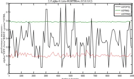
FSS model by ignoring uncertainties. In the hybrid strategy, the robust schedule is acquired from the robust optimization model (section 3.1) and RSH is implemented upon machine breakdown. In Figures 1 and 2, the results are reported for different problems' sizes and parameters. In these figures, AOFOPT, AOFRM, and
AOFPRM respectively represent the average objective function of the classical, robust, and proposed prediction methods. It can be concluded from Figures 1 and 2 that PRM outperforms the other two methods, no matter the problem size and parameters. According to Figures 1 and 2, there is a high difference between O.F. of the classical and robust schedules, also the classical schedule suffers from extreme fluctuations in O.F. versus uncertainties, so the scheduling should not be performed regardless of job processing time uncertainty even in a low degree of uncertainty. Also, it can be deduced from Figure 2 that job processing time uncertainty has a more decisive effect on O.F. than the machine failure rate. Since the
O.F. of PRM and RM are close to each other, given the cost of implementing the second step of the proposed algorithm, a manager can use a hybrid or the proposed predictive approach.
A case study. To indicate the applicability of the model it has been implemented on a real case in Petro Tajhiz Sepahan Company in Iran that specializes in designing and manufacturing various types of valves for the petrochemical industry. In summary, the functions of the valves are stopping/starting the fluid flow, varying its amount and controlling the direction of it. They are also used in regulation downstream systems, process pressure, relieving component and piping overpressure.
Figure 1. The comparison of the O.F. of OPT, RM and PRM
methods for the 2-machine 15 jobs problem, with a low degree of uncertainty, low failure rate, low MTTR, and coefficients (0.2, 0.3, 0.5) for efficiency, stability, and robustness
Figure 2. Comparison of the O.F. of OPT, RM and PRM
methods for the 2-machine 20 jobs problem, with a moderate degree of uncertainty, high failure rate, high MTTR, and coefficients (0.2, 0.3, 0.5) for efficiency, stability, and robustness
According to construction standards, valves are divided into five categories [24]. The case studied in this paper focuses on the production of two types of Forged Steel Valves. The production of the Forged Steel valves
is carried out via a flow shop system in six stages; Turning- Drilling- Grinding- Milling- Welding and Polishing. The production volume, the predetermined due dates and the processing times per stage are given in Table 1.
The first type of valves in this category are Needle Valves that can be used as a component for other valves. They are also used in fluid transmission lines, which include pharmaceuticals, foodstuffs, and chemicals. The second type of valves in this category is the Globe valve. In this type of valves, a disk moves perpen. The company receives orders from various oil/gas companies.
At the beginning of 2016, the company was contracted to construct and deliver eight orders. Due to the uncertain nature of the production, the processing times are defined via pessimistic, probable, and optimistic scenarios.
0 1000 2000 3000 4000 5000 6000 7000 8000 9000 10000
0 0.1 0.2 0.3 0.4 0.5 0.6 0.7 0.8
Number os Scenarios
p
e
r
f
o
r
m
a
c
e
m
e
a
s
u
r
e
=
a
lp
h
a
*
E
F
F
+
b
e
ta
*
R
B
S
T
+
g
a
m
a
*
S
T
B
L
2,15,alpha=0.1,teta=80,MTTRlow, (0.5,0.3,0.2)
AOFOPT(t) AOFRM(t) AOFPRM(t)
0 1000 2000 3000 4000 5000 6000 7000 8000 9000 10000
0 0.5 1 1.5 2 2.5 3
Number os Scenarios
p
e
rf
o
rm
a
ce
m
e
a
su
re
=
a
lp
h
a
*
E
F
F
+
b
e
ta
*
R
B
S
T
+
g
a
m
a
*
S
T
B
L
2,20,alpha=0.5,teta=60,MTTRligh,(0.5,0.3,0.2)
AOFOPT(t)
TABLE 1. The processing time of Forged Steel Valves under different scenarios*
*𝜆: Scenario, 𝑃𝜆: The probability of scenario 𝜆.
4. 1. Data Generation In this section, the obtained schedule from the proposed predictive algorithm and the empirical schedule in the company are compared with each other in terms of robustness, stability, and efficieny.
The processing times in the proposed method are uncertain, and they are estimated via a finite number of scenarios (Table 1). The processing times in the empirical method are the expected value of the processing time of all scenarios, i.e. 𝑡𝑖𝑗 = ∑ 𝑡𝑖𝑗𝜆𝑃𝜆 where
𝑡𝑖𝑗𝜆 is the processing time of 𝑗𝑡ℎjob on machine 𝑀𝑖 under scenario 𝜆 and 𝑃𝜆 is the occurrence probability of scenario 𝜆. In the proposed method, the time between consecutive breakdowns on the first machine is assumed to respectively follow an exponential distribution with the rates of 0.02, 0.0166 and 0.0125 for the optimistic, probable and pessimistic scenarios. Similar to Nouiri et
al., [7], the duration of the repair times follows an exponential distribution based on the meantime to repair value (MTTR) at two-level. The repair time duration is calculated via𝑡𝑟 = 𝑒𝑥𝑝 𝑟 𝑛𝑑(𝑀𝑇𝑇𝑅). The MTTR is calculated based on the machine busy time (MB); low level 𝑀𝑇𝑇𝑅𝑙∈ [0.01𝑀𝐵, 0.05𝑀𝐵] and high level
𝑀𝑇𝑇𝑅ℎ∈ [0.05𝑀𝐵, 0.1𝑀𝐵]. In the empirical method,
the reaction to breakdown is done by implementing the right shift rescheduling (RSH) policy to the affected jobs.
4. 2. The Empirical Schedule Procedure The company uses the following procedure to achieve an empirical schedule:
Step 1. The initial schedule generation.
The initial sequence of the jobs is determined according to the earliest due date rule (EDD) to minimize the total tardiness as an efficiency measure.
Step 2. Main Loop: for𝑠 = 1. . . 𝑁𝑠
Step 2.1. Random breakdown generation.
It is assumed that 𝜆″∈ 𝛺 is a real scenario. The random
breakdowns are generated according to the rate of breakdown in 𝜆″.
Step 2.2. Robustness, stability and efficiency.
The RSH is implemented upon a breakdown occurrence to obtain the actual (real) schedule. The robustness and stability measures are calculated with Equations (28) and (29), respectively.
4. 3. Robustness, Stability, Efficiency, and the Objective Function Suppose that 𝜆″∈ 𝛺 is the scenario that has actually happened. The robustness measure (𝑅𝑀) is defined as an absolute deviation of an efficiency measure (total tardiness) of the actual schedule from the initial one. It can be calculated via Equation (28), where ∑ 𝑇𝜆″
is the total tardiness of the actual schedule under scenario𝜆″∈ 𝛺, and ∑ 𝑇𝜆is the total
tardiness of the predictive schedule under scenario𝜆 ∈ 𝛺.
𝑅𝑀 = |∑ 𝑇𝜆″− ∑ 𝑇𝜆 𝑗
𝑗 | (28)
Moreover, stability measure (𝑆𝑀) is defined as an absolute deviation in job completion times (Equation 29), where 𝐶𝑚[𝑘]𝜆
″
is the completion time of the job in position
[𝑘] in the actual schedule under scenario 𝜆″∈ 𝛺, and
𝐶𝑚[𝑘]𝜆 is the completion time of the job in position [𝑘] in the predictive schedule under scenario 𝜆 ∈ 𝛺.
𝑆𝑀 = ∑ |𝐶𝑚[𝑘]𝜆
″
− 𝐶𝑚[𝑘]𝜆 | 𝑛
𝑘=1 (29)
Efficiency (Eff) is the measure of the optimality of the schedule. Here, the total completion time of the actual schedule is considered as an Efficiency measure.
𝐸𝑓𝑓 = ∑ 𝐶𝜆″
𝑗 (30)
The objective function is a multi-component measure based on the predefined measures of robustness, stability, and efficiency as follows (Equation 31).
Job Processing time per stage (min)
𝝀 𝑷𝝀 Valve 1 2 3 4 5 6
1 0.2 Needle 100 85 30 230 40 50
2 0.6 Needle 105 90 33 240 45 55
3 0.3 Needle 115 100 40 270 50 60
1 0.2 Gate 120 95 25 260 50 65
2 0.6 Gate 125 100 25 275 55 70
3 0.3 Gate 140 110 30 305 60 80
1 0.2 Check 55 45 25 125 25 35
2 0.6 Check 55 50 25 130 27 35
3 0.3 Check 60 55 30 145 30 40
1 0.2 Check 60 50 25 135 35 40
2 0.6 Check 65 54 25 145 35 40
3 0.3 Check 75 60 30 160 40 45
1 0.2 Check 65 75 25 155 35 35
2 0.6 Check 70 80 30 165 40 37
3 0.3 Check 80 90 35 185 45 40
1 0.2 Ball 155 125 35 400 50 10
2 0.6 Ball 167 135 40 417 55 10
3 0.3 Ball 183.7 148.5 44 458.7 60.5 11
1 0.2 Ball 190 175 55 455 60 20
2 0.6 Ball 200 185 58 480 65 20
3 0.3 Ball 220 203.5 63.8 528 71.5 22
1 0.2 Ball 250 260 60 550 70 25
2 0.6 Ball 265 273 65 580 75 30
𝑂. 𝐹. = 𝛼(𝑅𝑀) + 𝛽(𝑆𝑀) + 𝛾(𝐸𝑓𝑓) (31)
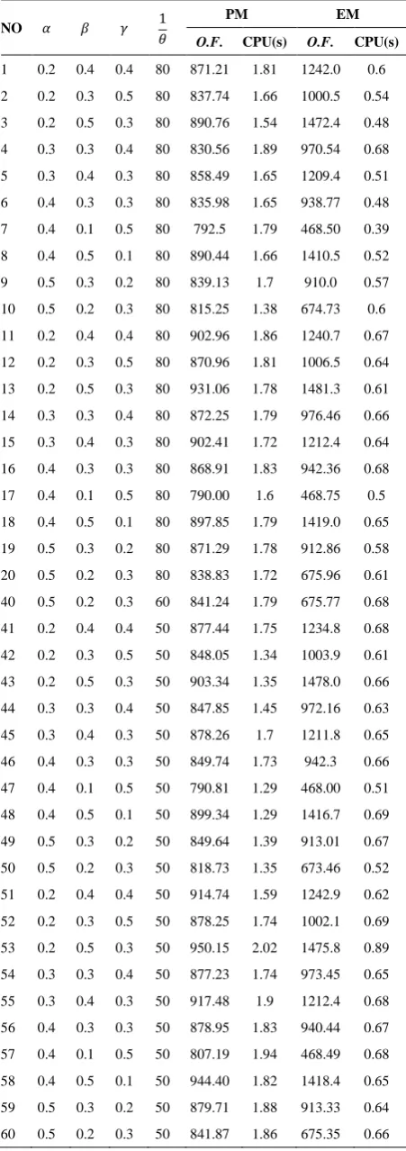
where 𝛼 + 𝛽 + 𝛾 = 1 and 𝛼, 𝛽, 𝛾 respectively indicate the degrees of importance of their corresponding objective. These parameters can be determined using methods such as sensitivity analysis, eigenvector, entropy, or the least-square method [1]. The proposed method (PM) and the empirical method (EM) can be compared concerning the value of O.F (Table 2). The calculations are made for different values of the coefficients at two levels of MTTR.
4. 4. Sensivity Analysis This section provides additional tests on the parameters of the model to gauge their effects on the value of the O.F.
4. 2. 1. Testing on the Time Interval Between Concequtive Breakdowns Figure 3 depicts the effect of different 1
𝜃on the value of the 𝑂. 𝐹. in the proposed method (PM). The dataset in the Figure 3 is derived from Table 2. From the problems with the low level of MTTR, instances 1 to 10, 21 to 30 and 41 to 50 are chosen that respectively correspond to values of 80, 60 and 50 for the interval between two consecutive failures.
In Figure 4, the notation OF-PM-80-L corresponds to the objective values found for the proposed method when 1
𝜃= 80 and the MTTR is set to the low level. As expected, in all the 10 instances of different categories, an increase in the average time between two failures improves the objective function, since the minimum values of the objective are achieved for 1
𝜃= 80.
4. 2. 2. Testing the Effect of MTTR Level In this section, the MTTR is first set to the low level (for the instances 1-10 in Table 2) and then set to the high level (instances 11- 20) to see the effect of its increment on the
O.F. The results are demonstrated in Figure 4. It can be seen in Figure 4 that an increase in MTTR, in turn, worsens the O.F. of the proposed method; ergo lower
MTTR levels are preferred.
Figure 3. The effect of different breakdown intervals on
the objective value
TABLE 2. The comparison between the O.F. of PM & EM
NO 𝛼 𝛽 𝛾 1
𝜃
PM EM
O.F. CPU(s) O.F. CPU(s) 1 0.2 0.4 0.4 80 871.21 1.81 1242.0 0.6
2 0.2 0.3 0.5 80 837.74 1.66 1000.5 0.54
3 0.2 0.5 0.3 80 890.76 1.54 1472.4 0.48
4 0.3 0.3 0.4 80 830.56 1.89 970.54 0.68
5 0.3 0.4 0.3 80 858.49 1.65 1209.4 0.51
6 0.4 0.3 0.3 80 835.98 1.65 938.77 0.48
7 0.4 0.1 0.5 80 792.5 1.79 468.50 0.39
8 0.4 0.5 0.1 80 890.44 1.66 1410.5 0.52
9 0.5 0.3 0.2 80 839.13 1.7 910.0 0.57
10 0.5 0.2 0.3 80 815.25 1.38 674.73 0.6
11 0.2 0.4 0.4 80 902.96 1.86 1240.7 0.67
12 0.2 0.3 0.5 80 870.96 1.81 1006.5 0.64
13 0.2 0.5 0.3 80 931.06 1.78 1481.3 0.61
14 0.3 0.3 0.4 80 872.25 1.79 976.46 0.66
15 0.3 0.4 0.3 80 902.41 1.72 1212.4 0.64
16 0.4 0.3 0.3 80 868.91 1.83 942.36 0.68
17 0.4 0.1 0.5 80 790.00 1.6 468.75 0.5
18 0.4 0.5 0.1 80 897.85 1.79 1419.0 0.65
19 0.5 0.3 0.2 80 871.29 1.78 912.86 0.58
20 0.5 0.2 0.3 80 838.83 1.72 675.96 0.61
40 0.5 0.2 0.3 60 841.24 1.79 675.77 0.68
41 0.2 0.4 0.4 50 877.44 1.75 1234.8 0.68
42 0.2 0.3 0.5 50 848.05 1.34 1003.9 0.61
43 0.2 0.5 0.3 50 903.34 1.35 1478.0 0.66
44 0.3 0.3 0.4 50 847.85 1.45 972.16 0.63
45 0.3 0.4 0.3 50 878.26 1.7 1211.8 0.65
46 0.4 0.3 0.3 50 849.74 1.73 942.3 0.66
47 0.4 0.1 0.5 50 790.81 1.29 468.00 0.51
48 0.4 0.5 0.1 50 899.34 1.29 1416.7 0.69
49 0.5 0.3 0.2 50 849.64 1.39 913.01 0.67
50 0.5 0.2 0.3 50 818.73 1.35 673.46 0.52
51 0.2 0.4 0.4 50 914.74 1.59 1242.9 0.62
52 0.2 0.3 0.5 50 878.25 1.74 1002.1 0.69
53 0.2 0.5 0.3 50 950.15 2.02 1475.8 0.89
54 0.3 0.3 0.4 50 877.23 1.74 973.45 0.65
55 0.3 0.4 0.3 50 917.48 1.9 1212.4 0.68
56 0.4 0.3 0.3 50 878.95 1.83 940.44 0.67
57 0.4 0.1 0.5 50 807.19 1.94 468.49 0.68
58 0.4 0.5 0.1 50 944.40 1.82 1418.4 0.65
59 0.5 0.3 0.2 50 879.71 1.88 913.33 0.64
60 0.5 0.2 0.3 50 841.87 1.86 675.35 0.66
785 805 825 845 865 885 905
1 2 3 4 5 6 7 8 9 10
o
b
je
ct
iv
e
fu
n
ct
io
n
sample number
Figure 4. The effect of the MTTR level on the O.F.
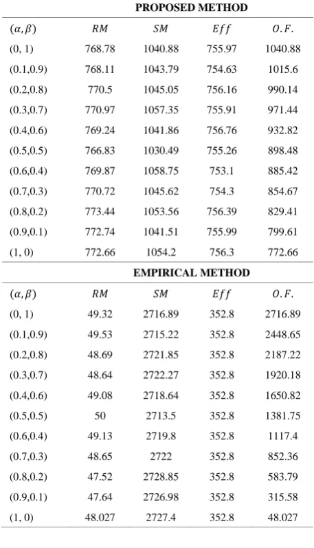
4. 2. 3. Testing on the Stability and Robustness Coefficients In this section, different values of the robustness and the stability coefficients (respectively
𝛼, 𝛽) are used to achieve the objective values of both PM
and EM. The results for the low level of MTTR, 𝜃 = 50
and𝛾 = 0 are summarized in Table 3.
The effects of the varying coefficients on O.F. are also depicted in Figure 5. According to Table 3 and Figure 5, the two methods perform similarly once 𝛼 = 0.7 and 𝛽 = 0.3. Before these values, PM is superior to the EM. Any more increase in the value of 𝛼and any more decrease in the value of 𝛽 worsen the O.F. of PM.
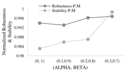
Ergo, if the emphasis is on the robustness of the schedule (𝛼 = 0, 𝛽 = 1), the proposed method is better. On the other hand, if a schedule with maximum stability is desired (𝛼 = 1, 𝛽 = 0), the empirical method is preferred. If a robust and stable schedule is required, then the proposed method should be picked since its range of superior performance is larger (𝛼 ≤ 0.7, 𝛽 ≥ 0.3). This shows the major impact of the coefficient on the performance, ergo the setting of these parameters should be carried out with care.There is a logical contradiction between stability and robustness since to enhance the schedule robustness, sequence manipulation may be necessary, which leads to stability degradation. To illustrate this conflict, the normalized data from Table 3 is used to plot Figure 6 to compare the stability and the robustness values of the proposed method.
4. 2. 4. Comparing the Effectiveness of the
Proposed and the Empirical Method According to the results of Table 2 and Figure 6, for both
levels of MTTR, and all values of 1
𝜃, the proposed method is more effective than the empirical one except in
(𝛼, 𝛽, 𝛾) = (0.4,0.1,0.5), and(𝛼, 𝛽, 𝛾) = (0.5,0.2,0.3).
hese results are confirmation of the major impact of the coefficient on the performance. As concluded from Figure 5, whenever a robust and stable schedule is required, then the proposed method should be selected since its range of superior performance is larger
(𝛼 ≤ 0.7, 𝛽 ≥ 0.3). Here, this conclusion becomes
more complete. That is, by choosing values more than 2 for the ratio of robustness to stability (𝛼
𝛽> 2), EM is the
preferred method and vice versa. Moreover, the trend of the objective values in the proposed method is smoother than its empirical counterpart. This difference is due to the robust optimization method used in the generation of the partial robust schedule.
TABLE 3. Comparison of the objective measures of the
proposed and empirical methods
PROPOSED METHOD
(𝛼, 𝛽) 𝑅𝑀 𝑆𝑀 𝐸𝑓𝑓 𝑂. 𝐹.
(0, 1) 768.78 1040.88 755.97 1040.88
(0.1,0.9) 768.11 1043.79 754.63 1015.6
(0.2,0.8) 770.5 1045.05 756.16 990.14
(0.3,0.7) 770.97 1057.35 755.91 971.44
(0.4,0.6) 769.24 1041.86 756.76 932.82
(0.5,0.5) 766.83 1030.49 755.26 898.48
(0.6,0.4) 769.87 1058.75 753.1 885.42
(0.7,0.3) 770.72 1045.62 754.3 854.67
(0.8,0.2) 773.44 1053.56 756.39 829.41
(0.9,0.1) 772.74 1041.51 755.99 799.61
(1, 0) 772.66 1054.2 756.3 772.66
EMPIRICAL METHOD
(𝛼, 𝛽) 𝑅𝑀 𝑆𝑀 𝐸𝑓𝑓 𝑂. 𝐹.
(0, 1) 49.32 2716.89 352.8 2716.89
(0.1,0.9) 49.53 2715.22 352.8 2448.65
(0.2,0.8) 48.69 2721.85 352.8 2187.22
(0.3,0.7) 48.64 2722.27 352.8 1920.18
(0.4,0.6) 49.08 2718.64 352.8 1650.82
(0.5,0.5) 50 2713.5 352.8 1381.75
(0.6,0.4) 49.13 2719.8 352.8 1117.4
(0.7,0.3) 48.65 2722 352.8 852.36
(0.8,0.2) 47.52 2728.85 352.8 583.79
(0.9,0.1) 47.64 2726.98 352.8 315.58
(1, 0) 48.027 2727.4 352.8 48.027
Figure 5. Effect of different stability and robustness
coefficients on the objectives
780 800 820 840 860 880 900 920
1 2 3 4 5 6 7 8 9 10
o
b
je
ct
iv
e
fu
n
ct
io
n
sample number
OF-PM-80-L OF-PM-80-H
0 500 1000 1500 2000 2500 3000
o
b
je
ct
iv
e
fu
n
ct
io
n
(robustness coificient, stability coificient)
Figure 6. The conflict between robustness and stability
5. CONCLUSION
In this paper, a robust and stable approach for scheduling the manufacturing lines in the valve production industry are presented. The problem is modeled as an uncertain
m-machine FSS system with machine breakdowns to optimize three performance measures; stability, robustness and efficiency, simultaneously. In the proposed approach, the problem is solved in two-stages. The first stage uses robust optimization to create a partial schedule by taking into account the uncertain processing times. Then the stability of the robust schedule is guaranteed faced with the new scenarios of job processing time. In the second stage, the appropriate buffer times were calculated via a linear programming model based on the defined performance measures in case of breakdowns of the first machine. The proposed predictive method is compared with reactive and hybrid approaches. In addition, the proposed predictive algorithm is applied to a real case from a valve company in Iran to investigate the superiority of this method over the empirical method currently used. The results showed that the proposed method is more adaptable to the occurrence of random events so that the variances in the objective values due to this change are much smoother than the empirical method. Ergo, this stable and robust schedule can increase the company's accountability to customers. The proposed model is formulated as an FSS
system in the valve-production industry.
In future researches, this model can be applied to other systems such as flexible flow shop or job shop systems, across similar industries. Moreover, our model is limited to the breakdown of the first machine. Depending on the corresponding industry, this model can be generalized to include the breakdowns of other machines as well. Another possibility for extending this work is to consider different probability distributions for the breakdown intervals or variable repair time.
6. REFERENCES
1. Rahmani, D., “A new proactive-reactive approach to hedge against uncertain processing times and unexpected machine
failures in the two-machine flow shop scheduling problems”,
Scientia Iranica, Vol. 24, No. 3, (2017), 1571–1584.
2. Goren, S. and Sabuncuoglu, I., “Optimization of schedule robustness and stability under random machine breakdowns and processing time variability”, IIE Transactions (Institute of Industrial Engineers), Vol. 42, No. 3, (2010), 203–220. 3. Al-Hinai, N. and Elmekkawy, T.Y., “Robust and stable flexible
job shop scheduling with random machine breakdowns using a hybrid genetic algorithm”, International Journal of Production Economics, Vol. 132, No. 2, (2011), 279–291.
4. Mehta, S. V. and Uzsoy, R. M., “Predictable scheduling of a job shop subject to breakdowns”, IEEE Transactions on Robotics and Automation, Vol. 14, No. 3, (1998), 365–378.
5. Gören, S., “Robustness and stability measures for scheduling policies in a single machine environment”, Doctoral dissertation, Bilkent University, Turkey, (2002)
6. Fazayeli, M., Aleagha, M.R., Bashirzadeh, R. and Shafaei, R., “A hybrid meta-heuristic algorithm for flowshop robust scheduling under machine breakdown uncertainty”, International Journal of Computer Integrated Manufacturing, Vol. 29, No. 7, (2016), 709–719.
7. Nouiri, M., Bekrar, A., Jemai, A., Trentesaux, D., Ammari, A.C. and Niar, S., “Two stage particle swarm optimization to solve the flexible job shop predictive scheduling problem considering possible machine breakdowns”, Computers and Industrial Engineering, Vol. 112, (2017), 595–606.
8. González-Neira, E.M., Montoya-Torres, J.R., and Barrera, D., “Flow-shop scheduling problem under uncertainties: Review and trends”, International Journal of Industrial Engineering Computations, Vol. 8, No. 4, (2017), 399–426.
9. Liao, W. and Fu, Y., “Min–max regret criterion-based robust model for the permutation flow-shop scheduling problem”,
Engineering Optimization, (2019), 1–14.
10. Framinan, J.M., Fernandez-Viagas, V. and Perez-Gonzalez, P., “Using real-time information to reschedule jobs in a flowshop with variable processing times”, Computers and Industrial Engineering, Vol. 129, (2019), 113–125.
11. Ma, S., Wang, Y. and Li, M., “A Novel Artificial Bee Colony Algorithm for Robust Permutation Flowshop Scheduling”, In Natural Computing for Unsupervised Learning, Springer, Cham, (2019), 163–182.
12. Amirian, H. and Sahraeian, R., “Multi-objective Differential Evolution for the Flow Shop Scheduling Problem with a Modified Learning Effect”, International Journal of Engineering, Transactions C: Aspects, Vol. 27, No. 9, (2014), 1395–1404. 13. Mokhtari, H., Molla-Alizadeh, S. and Noroozi, A., “A Reliability
based Modelling and Optimization of an Integrated Production and Preventive Maintenance Activities in Flowshop Scheduling Problem”, International Journal of Engineering - Transactions C: Aspects, Vol. 28, No. 12, (2015), 1774–1781.
14. Tavakkoli-Moghaddam, R., Lotfi, M.M., Khademi Zare, H. and Jafari, A. A., “Minimizing Makespan with Start Time Dependent Jobs in a Two Machine Flow Shop”, International Journal of Engineering - Transactions C: Aspects, Vol. 29, No. 6, (2016), 778–787.
15. Kouvelis, P., Daniels, R.L., and Vairaktarakis, G., “Robust scheduling of a two-machine flow shop with uncertain processing times”, IIE Transactions (Institute of Industrial Engineers), Vol. 32, No. 5, (2000), 421–432.
16. Rahmani, D. and Heydari, M., “Robust and stable flow shop scheduling with unexpected arrivals of new jobs and uncertain processing times”, Journal of Manufacturing Systems, Vol. 33, No. 1, (2014), 84–92.
17. Cui, W., Lu, Z., Li, C. and Han, X., “A proactive approach to solve integrated production scheduling and maintenance planning
0.98 0.984 0.988 0.992 0.996 1
(0, 1) (0.1,0.9) (0.2,0.8) (0.3,0.7)
N
o
rmal
iz
ed
R
o
b
u
st
n
ess
&
S
ta
b
il
it
y
(ALPHA, BETA)
problem in flow shops”, Computers and Industrial Engineering, Vol. 115, (2018), 342–353.
18. Briskorn, D., Leung, J. and Pinedo, M., “Robust scheduling on a single machine using time buffers”, IIE Transactions (Institute of Industrial Engineers), Vol. 43, No. 6, (2011), 383–398. 19. Mulvey, J.M., Vanderbei, R.J. and Zenios, S.A., “Robust
Optimization of Large-Scale Systems”, Operations Research, Vol. 43, No. 2, (1995), 264–281.
20. Chaari, T., Chaabane, S., Loukil, T., and Trentesaux, D, “A genetic algorithm for robust hybrid flow shop scheduling”,
International Journal of Computer Integrated Manufacturing, Vol. 24, No. 9, (2011), 821–833.
21. Yu, C.S. and Li, H.L., “Robust optimization model for stochastic logistic problems”, International Journal of Production Economics, Vol. 64, No. 1–3, (2000), 385–397.
22. Pinedo, M. and Hadavi, K., “Scheduling: Theory, Algorithms and Systems Development”, In Operations Research Proceedings, Springer Berlin Heidelberg, (1992), 35–42.
23. Gan, H.S. and Wirth, A., “Comparing deterministic, robust and online scheduling using entropy”, International Journal of Production Research, Vol. 43, No. 10, (2005), 2113–2134. 24. Zappe, R.W., Valve selection handbook, Gulf Professional
Publishing, (1999)..
A New Approach Generating Robust and Stable Schedules in
m-Machine Flow Shop
Scheduling Problems: A Case Study
Z. Abtahia, R. Sahraeiana, D. Rahmanib
a Department of Industrial Engineering, College of Engineering, Shahed University, Tehran, Iran b Department of Industrial Engineering, K.N. Toosi University of Technology, Tehran, Iran
P A P E R I N F O
Paper history: Received 12 March 2019
Received in revised form 10 October 2019 Accepted07November 2019
Keywords:
Machine Breakdowns Robustness Scheduling Stability
Uncertain Flow Shop System
هدیکچ هصلاخ رد نیا هلاقم کی هلئسم نامز ی یدنب اب نامز شزادرپ یعطقریغ و یبارخ نیشام رد طیحم یاه یتعنص ای یرادا رد رظن هتفرگ هدش و اب هدافتسا زا کی شور دیدج هنیهب یزاس مواقم لح تسا هدش . رد یاهشور هنیهب یزاس ،مواقم تمواقم لح طقف یارب هعومجم یاهویرانس رد رظن هتفرگ هدش ظفح یم دوش هک نکمم رد تسا ربارب یاهویرانس دیدج رتدب دوش . رد نیا هلاقم ، کی متیروگلا شیپ هنانیب ود ی هلحرم یا هئارا هدش تسا هک رداق هب شنکاو رثوم هب مدع تیعطق اه و دیلوت لح یاه مواقم و رادیاپ تسا . رد هلحرم ،متیروگلا لوا نامز
و دیلوت مواقم یدنب نآ یرادیاپ رد ربارب یاهویرانس دیدج نیمضت یم دوش . رد هلحرم ،مود کی یارب دیدج سایقم یرادیاپ
هئارا هدش نامز رب نیشام یبارخ رثا هک تسا هلحرم مواقم یدنب
ی
یم لیدعت ار لبق هولاع .دنک رب ،نیا نامز کی یفاک طرش یدنب عقاو ،هنانیب هدروآرب ندرک مه نامز یاهزاین ،یرتشم هدننکدیلوت و نانکراک تسا . نیا رد اب ،هلاقم فیرعت کی سایقم هس زا هناگ ،ییآراک ،تمواقم و یرادیاپ هب نیا یم هتخادرپ مهم دوش
.
فیرعت لیوحت یاهدعوم و اهراک ریخات یعقاو نامز عومجم ساسا رب تمواقم سایقم ،یرتشم تامازلا ندرک هدروآرب یارب
رد .تسا هدش ،نایاپ متیروگلا یداهنشیپ رد کی هعلاطم یدروم هب هدش هتفرگ راک و درکلمع نآ اب شور یبرجت تکرش هسیاقم یم دوش . جیاتن یتابساحم یکاح زا یرترب شور یبرجت شور هب یداهنشیپ رد حطس دوبهب تیاضر نایرتشم ، نانکراک و یروآدوس شیازفا و ییوگخساپ هناخراک یم دشاب .