Gabriel Caloz & Monique Dauge, Editors
A LOOK AT HOW LDG AND BEM CAN BE COUPLED
∗,∗∗Rommel A. Bustinza
1, Gabriel N. Gatica
1and Francisco–Javier Sayas
2Dedicated to Michel Crouzeix, admired ‘maestro’ of Numerical Analysis
Abstract. In this work we explain the coupling of Local Discontinuous Galerkin and general Bound-ary Element methods for a class of nonlinear exterior transmission problems. The method is exposed as the discrete coupling of two Neumann–to–Dirichlet operators, one coping with all nonlinearities and source terms and the other for a purely exterior Laplace equation. We show how two separate methods for interior and exterior problems can be coupled at a weak level using a mortar space and how the analysis can be organised with very little interaction of the interior and exterior parts by considering the natural seminorms to measure the influence of the coupling unknown on the different methods.
Introduction
The coupling of Finite and Boundary Element methods goes three or four decades back in the not–so–long history of Numerical Analysis. At the present moment when Numerical Analysis and Scientific Computation tend to run in parallel, these coupling procedures offer a possibility to numerical analysts of taking the standpoint of practitioners while keeping the focus in mathematics and also of enjoying the perspective of developing strategies to use different numerical packages together with minimum effort in recoding. Although the basic coupling procedures for finite and boundary elements were already developed in the seventies, new rewritings of them allow to use old ideas of Schwarz iterations to devise practical implementations with little interaction between both numerical methods. In more recent efforts to understand and solve multiphysics problems, it seems now more important than ever to be able to use different methods, specialised for different problems, together in a single code. In this line, we are going to sketch here how to couple Locally Discontinuous Galerkin methods with Boundary Element Methods.
The coupling of FEM and BEM is usually employed when dealing with problems in the whole space or outside a bounded domain, when all the difficulties (inhomogeneities, sources, nonlinearities) happen in a bounded region outside of which the problem is a simple linear homogeneous PDE with constant coefficients and a certain prescribed behaviour at infinity (be it an energy finiteness condition or a radiation condition). The method works by imposing an artificial boundary surrounding all the difficult elementsof the problem, thus creating a false transmission problem. Sometimes, the artificial interface is taken to be a physical interface
∗Research of R.A. Bustinza and G.N. Gatica partially supported through FONDECYT Projects 1050842 and 7050209 and the FONDAP Program in Applied Mathematics.
∗∗Research of F.–J. Sayas is partially supported by FEDER/MCYT Project MTM2004-01905 and Gobierno de Arag´on (Grupo Consolidado PDIE)
1 GI2MA, Departamento de Ingenier´ıa Matem´atica, Universidad de Concepci´on, Casilla 160–C, Concepci´on, Chile 2 Departamento de Matem´atica Aplicada, CPS, Universidad de Zaragoza, 50018 Zaragoza, Spain
c
if there is a clear–cut option, for instance, when there is a real transmission problem (as in wave–structure interaction problems) or when the nonlinearities or inhomogeneities happen in a domain which is simple enough for numerical purposes. Thus we end up with: (a) a boundary value problem in a bounded domain, with possible variable coefficients, nonlinear terms or sources and with no prescribed boundary condition in the artificial interface, which is part of its boundary; (b) a linear homogeneous PDE with constant coefficients (typically a Laplace, Helmholtz, Lam´e or Maxwell equation) on the exterior of the artificial boundary, on which no boundary condition is prescribed and with some radiation condition at infinity; (c) some transmission conditions coupling both parts of the problem. Part (a) of the problem can be then numerically approximated with any variant of FEM (conforming, nonconforming, mixed), whereas part (b) can be approximated with BEM. The main point now is how we can impose the transmission conditions to couple both numerical methods. The first tries at this problem involved a very close coupling of the method, with the different discrete spaces interacting with each other. For the classical model problems (exterior BVP of second order) the different options were motivated by questions related to compactness (or lack thereof) of some integral operator appearing in the boundary integral formulation of the exterior–most part. In the mathematical community the original references for the proposal and analysis of the coupling procedures using a single integral equation (and here compactness of the aforementioned operator was relevant) are the papers of Johnson and N´ed´elec [8] and of Brezzi and Johnson [2]. When that compactness property failed (with non–smooth artificial interfaces and also in elasticity problems), two equations had to be used and the ellipticity of the exterior problem was used not only at the continuous level but also at the discrete one. The papers of Costabel [5] and Han [7] offered the solution. We also would like to mention that the engineering literature was very fast to recognise the interest of coupling finite and boundary elements, as can be inferred from the early date of [10].
For simplicity of exposition we will restrict our interest to a three dimensional problem on the exterior of a Lipschitz polyhedron. Full details of the analysis (in the two–dimensional setting however) appear in [6] for the linear case and in [4] for the non–linear one. We will cover here the nonlinear situation to benefit from the localization advantages of Discontinuous Galerkin methods. Among these we will deal with the Locally Discontinuous Galerkin method, although the coupling strategy can be adapted to some other schemes which share many common features with this one. For a complete taxonomy of DG methods, applied to elliptic problems, exploring and explaining similarities and differences between them, we refer to the excellent exposition in [1]. Exposition will be narrative in style. Proofs can be found in [6] or [4] or follow from relatively simple modifications of arguments therein. We will follow the following plan in four sections: first we formulate the problem as the matching of one interior and one exterior solvers; then we explain the exterior BEM solver; thirdly we explain the interior LDG solver; in the final section we sketch the ideas behind coupling and its analysis, having everything well prepared from the preceding sections.
1.
Matching of Neumann–to–Dirichlet operators
Let Ω0be a bounded Lipschitz polyhedron inR3, with boundary Γ0. We want to solve the following problem, outside Γ0:
diva(·,∇ω) +f = 0, in ext Ω0,
ω=g0, on Γ0,
ω=uinc+o(1), at infinity.
The required regularity is simply local H1 behaviour, which imposes that the data functiong0 must belong to
H1/2(Γ0) for the problem to make sense. The main feature of the flux functiona is that there exists another Lipschitz polyhedral boundary Ξ such that
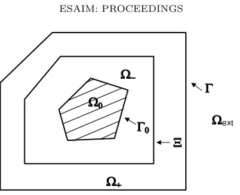
Figure 1. The geometrical setting of the problem in a simplified two–dimensional view.
that is to say, the problem is simply a Poisson equation outside Ξ. The function uinc is assumed to be smooth and to satisfy ∆uinc = 0 in ext Ξ. Also we assume that f ≡0 except on a bounded region, where it is square integrable. Then we create a new polyhedral boundary Γ that surrounds both Ξ and the support of f. This new interface, creates three zones: the interior nonlinear region Ω−, the nonhomogeneous linear region Ω+ and the exterior region Ωext (See Figure 1 for a two–dimensional cartoon of the geometrical setting).
Conditions on the flux function a are: the usual Carath´eodory conditions sufficient for the corresponding Nemitskii operators to be defined, two growth conditions
|a(x, θ)| ≤C1|θ|+C2(x), |Dθa(x, θ)| ≤C3, C2∈L2(Ω−),
and the ellipticity condition
Dθa(x, θ)·θ≥C4|θ|2, C4>0. All conditions are assumed to hold for arbitraryθalmost everywhere in x.
The first thing we do is taking the incident solution (the one defining behaviour at infinity) out of the problem. To do that we define the exterior Cauchy data ofuinc on Ξ
g1:=uinc|+Ξ, g2:=∂νuinc|+Ξ
and assume the second one to be inL2(Ξ). Then we take as new unknown
u:=
(
ω, in Ω−,
ω−uinc, in Ω+∪Ωext.
From the point of view of the transmission interface Γ, we have two different problems. The coupling unknown will be
λ:=∂νu=∂νω−∂νuinc: Γ→R.
Theinterior problemis simply set by solving (we write Ω := Ω−∪Ξ∪Ω+)
ω∈H1(Ω), ω|Γ0 =g0, Z
Ω
a(·,∇ω)· ∇v=
Z
Ω
f v+
Z
Γ
(λ+∂νuinc)v, ∀v∈H1(Ω), v|Γ0 = 0.
(1)
This is a strongly monotone Lipschitz problem that admits a unique solution. The operator that associates
will be denoted NtDint, as short for Neumann–to–Dirichlet for the interior domain. Ifuis taken as the unknown, the problem is more complicated, becoming the weak formulation of
u=g0, on Γ0
diva(·,∇u) +f = 0, in Ω−,
u−−u+=g
1, on Ξ,
∂−
νu−∂ν+u=g2, on Ξ, ∆u+f = 0, in Ω+,
∂νu=λ, on Γ,
(2)
but the operator NtDint:H−1/2(Γ)→H1/2(Γ) is more simply written as
∂νu=:λ7−→ϕ:=u.
The solution to theexterior problemcan be expressed by means of layer potentials, using the well–known representation formula (also called Green’s third theorem, see [9])
u=Dϕ− Sλ:=
Z
Γ
∂ν(y)
1 4π| · −y|
ϕ(y) dγ(y)− Z
Γ
λ(y)
4π| · −y|dγ(y)
(as beforeλ=∂νuandϕ=u). The four boundary integral operators on Γ will be denoted
V λ=
Z
Γ
λ(y)
4π| · −y|dγ(y), Kϕ= Z
Γ
∂ν(y)
1 4π| · −y|
ϕ(y) dγ(y),
K′λ=
Z
Γ
∂ν(·)
1 4π| · −y|
ϕ(y) dγ(y), W ϕ=−∂ν
Z
Γ
∂ν(y)
1 4π| · −y|
ϕ(y) dγ(y).
Using the jump relations of potentials we can write that up to a constant
ϕ=−W−1(12I+K′)λ,
since the operatorW−1is elliptic, and therefore invertible, on the space H1/2
0 (Γ) :={ϕ∈H1/2(Γ)|
R
Γϕ= 0}. Ignoring the additional constant thatW−1is not able to recuperate, the exterior Neumann–to–Dirichlet operator admits an integral formulation−W−1(1
2I+K
′).Although bothW−1(1 2I+K
′) andW−1are elliptic, a numerical method based upon numerically inverting W needs the compactness ofK′ to stay stable. This property, in its turn, needs a certain amount of regularity on Γ, that does not hold true if Γ is polyhedral. It is then more adequate to duplicate λ, both as datum and unknown, in the symmetric elliptic boundary integral system
W ϕ − (12I−K′)γ = −λ,
(1
2I−K)ϕ + V γ = 0,
(3)
which gives
W + (12I−K′)V−1(12I−K)ϕ=−λ
and thus, an alternative expression for the exterior Neumann–to–Dirichlet operator
NtDext=− W+ (1 2I−K
′)V−1(1 2I−K)
−1
A typical Galerkin discretization of (3) profits from the symmetric elliptic structure of the problem also at the discrete level. This will be the departure point for the numerical scheme.
Thecoupled problemconsists of takingλas unknown and making the exterior and interior NtD operators match
NtDint(λ)−NtDext(λ) = 0. (4)
This problem can again be proven to be Lipschitz strongly monotone inH−1/2(Γ) and therefore has a unique solution.
The point of view of considering the interior problem as the main problem and incorporating the operator NtDext as a nonlocal boundary condition is the typical frame of exact Absorbing Boundary Conditions. An-alytical or numerical approximations of NtDext give then rise to different approaches to solve the problem. If the bounded domain is composed of several disconnected regions, small with respect to the whole size of the problem, the point of view is logically closer to that of scattering problems, and the interior NtD operator acts as the action of some kind of scatterer in a phenomenon happening in free space. Finally, equalling the impor-tance of both NtD operators and taking (4) as a fixed point equation gives rise to different types of Schwarz or Neumann–Schwarz iterations (domain decomposition without overlapping). Even if these iterations are not likely to converge, they can be used as departure point for Krylov iterations, since these can be used even at the non–discrete level of equation (4).
2.
Boundary element block
To approximate (3) we choose two sequences of boundary element spaces
Yh⊂H1/2(Γ), Zh⊂H−1/2(Γ)
and set the Galerkin equations: findϕh∈Yh,γh∈Zh such that
hW ϕh, φhi − h(12I−K′)γh, φhi = −hλ, φhi, ∀φh∈Yh
h(12I−K)ϕh, ηhi + hV γh, ηhi = 0, ∀ηh∈Zh.
(5)
These equations give rise to the exterior discrete NtD operator
NtDexth :H−1/2(Γ)→Yh, NtDexth (λ) :=ϕh.
Defining the seminorm,
|λ|h,ext:= sup φh∈Yh
hλ, φhi
kφhk1/2,Γ
≤ kλk−1/2,Γ, (6)
it can be proven that
|hη,NtDexth (λ)i|.|η|h,ext|λ|h,ext, −hλ,NtDexth (λ)i&|λ|2h,ext (7)
(the symbols.and&are henceforth used to avoid writing down constants independent of the discrete parameter
hand of the solution and data of the problem).
3.
Discontinuous Galerkin block
To approximate (2) we will use a LDG method, as proposed for nonlinear problems in [3]. The first point consists of taking three unknowns
u, θ:=∇u, σ:=a(·, θ)
begin with a usual tetrahedral mesh and then perform an asymptotically limited number of element refinements, preserving shape regularity but losing the complete matching of faces). On each tetrahedron K we choose a scalar–valued polynomial spaceP(K) and a vector–valued polynomial spaceP(K). The polynomial degree in different elements is allowed to differ but has to be kept asymptotically bounded. We also have to demand that
∇P(K)⊂P(K).
The discrete equations are defined element by element. Upon determination of the numerical flux operators (we will do it in short) that create the necessary interelement connections and impose the boundary and transmission conditions, the discrete equations look for uK ∈ P(K) and θK, σK ∈ P(K) satisfying a discrete version of the state equationa(·, θ) =σ
Z
K
a(·, θK)·ζK−
Z
K
σK·ζK= 0, ∀ζK ∈P(K), (8)
a discrete weak version of the relation∇u=θ Z
K
uKdivτK+
Z
K
θK·τK−
Z
∂Kb
u∂KτK·ν= 0, ∀τK∈P(K), (9)
and the discrete version of the equilibrium equation divσ+f = 0
Z
K
σK· ∇vK−
Z
∂K
(bσ∂K·ν)vK=
Z
K
f vK, ∀vK ∈P(K). (10)
Notice that interelement connections appear in equations (9) and (10), which are linear, and that the nonlinear equation (8) is isolated element by element.
Following [1], fluxes on the element boundaries can be introduced through a clever definition of average and jump operators on the faces of the triangulation. Faces of elements are counted only once, but seen from the smallest element to which they belong (therefore, a tetrahedron can have more than four faces if one of its real faces is subdivided from the exterior because it touches more that one tetrahedron on that side). We then write
Eh:=Ehint∪ EΓ
0
h ∪ E Ξ,−
h ∪ E Ξ,+ h ∪ E
Γ h
to the respective lists of faces interior to Ω−∪Ω+, faces on Γ0, faces on Ξ seen from Ω−, faces on Ξ seen from
Ω+ and faces on Γ.
Two sets of constant coefficients on faces (the space of constant functions oneis denotedP0(e))
α∈Y{P0(e)|e∈ Ehint∪ EΓ
0
h ∪ E Ξ,−
h ∪ E Ξ,+
h }, β ∈
Y
e∈Eint h
P0(e)
3
,
satisfying
|βe|.1, 1.αehe.1,
are needed to define the numerical fluxes of the LDG method. Denoting then
L2(Eh) := Y e∈Eh
L2(e), H1(Th) := Y K∈Th
H1(K),
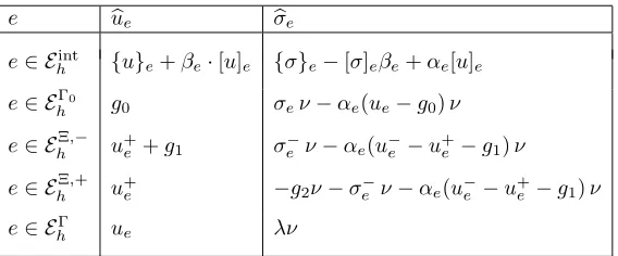
the numerical fluxes are the operators
b
u:H1(Th)×L2(Γ0)×L2(Ξ) −→ L2(Eh)
e bue bσe
e∈ Eint
h {u}e+βe·[u]e {σ}e−[σ]eβe+αe[u]e
e∈ EΓ0
h g0 σeν−αe(ue−g0)ν
e∈ EhΞ,− u+
e +g1 σe−ν−αe(u−e −u+e −g1)ν
e∈ EhΞ,+ u+e −g2ν−σe−ν−αe(u−e −u+e −g1)ν
e∈ EΓ
h ue λν
Table 1. Numerical fluxes for the LDG block
and
b
σ:H1(Th)×H1(Th)3×L2(Γ
0)×L2(Ξ)×L2(Ξ)×L2(Γ) −→
L2(Eh)3
(u, σ, g0, g1, g2, λ) 7−→ σb
defined by the expressions in Table 3
The LDG equations (8–10) admit several possible global rewriting, each one emphasizing a particular aspect of the method. Following [3] we will write down a non–consistent global primal form of the equations, instead of the consistent reformulation of [1]. The global spaces are
uh∈Vh:=
Y
K∈Th
P(K), θh, σh∈Σh:=
Y
K∈Th P(K).
The piecewise gradient operator∇h:H1(Th)→
L2(Th)]3is naturally corrected by the numerical fluxes in the form of a corrected discrete gradient∇∗
h:H1(Th)→Σh defined by the equations
Z
Ω
∇∗hv·τh =
Z
Ω
∇hu·τh
+ X
e∈Eint h
Z
e
[v]· {τh} −[τh]β
+
Z
Γ0
v(τh·ν) +
Z
Ξ
(v−−v+) (τh−·ν), ∀τh∈Σh.
Since the Dirichlet condition (and the first transmission condition, which is also of Dirichlet type) appear inside the numerical fluxes, we need an artificial vector–lifting of them: gh∈Σh, such that
Z
Ω
gh·τh=
Z
Γ0
g0(τh·ν) +
Z
Ξ
g1(τh−·ν), ∀τh∈Σh.
Obviously, this lifting appears only in the non–linear part, since the choice in the definition of the numerical fluxes has been to consider the physical interface Ξ as a Dirichlet boundary from inside. As usual in Discontinuous Galerkin methods, a bilinear form that penalizes interelement jumps is definedα:H1(Th)×H1(Th)→R
α(u, v) := X e∈Eint
h
αe
Z
e
[u]·[v] +
Z
Γ0 α u v+
Z
Ξ
Finally, we consider a semilinear formβh:H1(Th)×H1(Th)→R
βh(u, v) :=
Z
Ω
a(·,∇∗hu+gh)· ∇∗hv+α(u, v)−
Z
Ω
f v− Z
Γ0
αg0v−
Z
Ξ
α g1(v−−v+)−
Z
Ξ
g2v+
=
Z
Ω
a(·,∇∗
hu+gh)· ∇∗hv−
Z
Ω
f v− Z
Ξ
g2v++
X
e∈Eint h
αe
Z
e [u]·[v]
+
Z
Γ0
α(u−g0)v+
Z
Ξ
α(u−−u+−g1) (v−−v+).
The equations of the LDG method admit then the simple following reformulation. The unknown uh is the solution to the problem: find uh∈Vh such that
βh(uh, vh) =
Z
Γ
λ vh, ∀vh∈Vh. (11)
The discrete gradient is the corrected gradient of the numerical solution plus the lifting of the Dirichlet conditions
θh=∇∗huh+gh
and the discrete flux is simply theL2(Ω)−projection onto Σh of the flux created by the numerical solution
Z
Ω
σh·τh=
Z
Ω
a(·, θh)·τh, ∀τh∈Σh.
In the discrete norm (defined inH1(Th)
|||u|||2h:=
Z
Ω
|∇hu|2+α(u, u),
the semilinear form of problem (11) satisfies
|βh(u, v)−βh(w, v)|.|||u−w|||h|||v|||h, βh(u, u−v)−βh(v, u−v)&|||u−v|||2h, ∀u, v, w∈H1(Th)
and therefore these equations are uniquely solvable for arbitraryλ. The interior NtD operator is given by
NtDinth :H−1/2(Γ)→VhΓ, NtDinth (λ) :=uh, on Γ,
whereVhΓ is the space of restrictions of elements ofVhto Γ.
Writing the equivalent relations to (7) for the interior discrete NtD operator requires the introduction of the corresponding natural seminorm for the right–hand sides of (11). To do that we consider the optimal lifting norm onVhΓ:
kηhkh,Γ:= inf
|||vh|||h
vh=ηh on Γ and the seminorm
|λ|h,int := sup ηh∈VhΓ
hλ, ηhi
kηhkh,Γ
.kh−1/2λk
0,Γ, (12)
With respect to this seminorm, the properties of NtDinth can be written in a very straightforward way (the price is, of course, the difficulty of correctly understanding the seminorm): for all λ, µ, ρ∈L2(Γ)
4.
Discrete coupling
Since both interior and exterior NtD operators are already set, we simply have to couple both operators and demand that they give approximately the same solution. Notice that the exterior operator proceeding from a Galerkin discretization, NtDexth (λ) is a continuous function in a spaceYh defined on a boundary grid on Γ (it can even be a function on a discrete space that has nothing to do with the finite element philosophy), whereas NtDinth (λ) belongs to a non–conforming (discontinuous) finite element space on Γ, the one inherited by restricting elements ofVh to this boundary. Note that these spaces need not even to have the same dimension. Then we choose an additional spaceXh, a priori independent of both existing discretizations on Γ, which will act as a mortar space. The coupled equations are a set of Galerkin equations to equate both DtN operators, i.e., a Galerkin discretization of (4): findλh∈Xh such that
hNtDinth (λh)−NtDexth (λh), µhi= 0, ∀µh∈Xh.
Notice that the spaceXh meetsYh (a BEM space) andVhΓ (the trace of a LDG space) simply inL2(Γ)−inner products in the coupled equations, but that the BEM and LDG spaces do not meet each other in any term.
Denoting
|λ|2h:=|λ|2h,int+|λ|2h,ext, it is simple to check that the semilinear form
Ah(λ, µ) :=hNtDinth (λ)−NtDexth (λ), µi
satisfies for allλ, µ, ρ∈L2(Γ)
|Ah(λ, µ)− Ah(ρ, µ)|.|λ−ρ|h|µ|h, Ah(λ, λ−µ)− Ah(µ, λ−µ)&|λ−µ|2h.
Assuming that| · |his a norm, this guarantees existence and uniqueness of solution to the coupled system. This condition imposes that the mortar space cannot be too rich in comparison to at least one ofYh andVhΓ (see the definitions of| · |h,int and| · |h,ext). The first rough estimate follows from general theory of approximation of strongly monotone Lipschitz operators:
|λ−λh|h. inf µh∈Xh
|λ−µh|h+ sup 06=µh∈Xh
|Ah(λ, µh)| |µh|h
. (13)
Notice that the error in all the relevant quantities in the coupled system (uh, θh, σh, ϕh, γh) can be bounded from above in their natural norms by the term |λ−λh|h. The first term in the right–hand side of (13) is an approximation error, that can be easily bounded for many particular choices of Xh using the upper bounds in (6) and (12) and profiting from the fact that λ∈ C∞(Γ). The second term in (13) is a consistency term,
due to the fact that the exact solution does not satisfy the discrete equations (as they are written in primal form!). We emphasize again that the primal form of the LDG method is an extension to a wider space of the discrete equations. The original discrete equations (8, 9, 10) are defined on a space of discontinuous piecewise polynomial functions. In that formulation the discrete set of equations is consistent: when the exact solution (assumed to be smooth enough) is input into the equations, it produces no residual. However, these discrete equations can be rewritten in the primal form shown above and this new formulation, which we use for the sake of analysis, is inconsistent: the exact solution leaves now residual when input into the equations.
The consistency term admits the following bound:
|Ah(λ, µh)| ≤ |hNtDinth (λ)−NtDint(λ), µhi|+|hNtDext(λ)−NtDexth (λ), µhi|
≤
ε1(h)kh1/2(u−uh)k0,Γ+ε2(h)kϕ−ϕhk1/2,Γ
where the quantities
ε1(h) := sup 06=µh∈Xh
kh−1/2µ hk0,Γ
|µh|h,int
, ε2(h) := sup
06=µh∈Xh
kµhk−1/2,Γ
|µh|h,ext
are a measure of the degree of tightness of the bounds in (6) and (12). That these quantities do not degenerate (or do not degenerate strongly) ashdecreases depends on the equilibrium betweenXhand the boundary spaces that it meets in the coupled equations, i.e., Yh and VhΓ. The remaining terms in the consistency error are separate error bounds for the LDG and BEM methods assuming that all the data (in particular, the coupling unknown λ) is known. A particular choice of spaces where the analysis can be carried out to the very end is given in [4].
References
[1] D. N. Arnold, F. Brezzi, B. Cockburn, and L. D. Marini. Unified analysis of discontinuous Galerkin methods for elliptic problems.SIAM J. Numer. Anal., 39(5):1749–1779 (electronic), 2001/02.
[2] F. Brezzi and C. Johnson. On the coupling of boundary integral and finite element methods.Calcolo, 16(2):189–201, 1979. [3] R. Bustinza and G. N. Gatica. A local discontinuous Galerkin method for nonlinear diffusion problems with mixed boundary
conditions.SIAM J. Sci. Comput., 26(1):152–177 (electronic), 2004.
[4] R. Bustinza, G. N. Gatica, and F.-J. Sayas. On the coupling of local discontinuous Galerkin and boundary element methods for nonlinear exterior transmission problems. To appear in IMA J. Numer. Anal.
[5] M. Costabel. Symmetric methods for the coupling of finite elements and boundary elements. InBoundary elements IX, Vol. 1 (Stuttgart, 1987), pages 411–420. Comput. Mech., Southampton, 1987.
[6] G. N. Gatica and F.-J. Sayas. An a priori error analysis for the coupling of local discontinuous Galerkin and boundary element methods.Math. Comp., 75:1675–1696, 2006.
[7] H. D. Han. A new class of variational formulations for the coupling of finite and boundary element methods.J. Comput. Math., 8(3):223–232, 1990.
[8] C. Johnson and J.-C. N´ed´elec. On the coupling of boundary integral and finite element methods.Math. Comp., 35(152):1063– 1079, 1980.
[9] W. McLean.Strongly elliptic systems and boundary integral equations. Cambridge University Press, Cambridge, 2000. [10] O. C. Zienkiewicz, D. W. Kelly, and P. Bettess. The coupling of the finite element method and boundary solution procedures.